Magnetic properties of the lattice Anderson model - Department of ...

Magnetic properties of the lattice Anderson model
H. Q. tin
Department of Physics, University of Illinois at Urbana-Champaign, Urbana, Illinois 61801
H. Chen
Cray Research, Inc., Minneapolis, Minnesota 55121
J. Callaway
Department of Physics, Louisiana State University, Baton Rouge, Louisiana 70803-4001
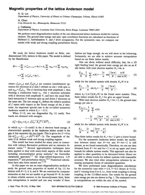
We perform exact diagonalization studies of the one-dimensional lattice Anderson model for various
clusters. The ground state energy and spin-spin correlation functions are calculated as functions of
Hubbard U, hybridization V, and f level occupancies. For the symmetric case, we compare our
results with weak and strong coupling perturbation theory.
We study the lattice Anderson model on finite, onedimensional
(lD), lattices in this paper. The model is defined
by the Hamiltonian
H=-tC (c~&+,,+hc)+EfC ntia+uC rlfiplfil
io ia i
+vC (cTJic+hc) P (1)
ia
where ci&ci,) and fio(fi,) are creation (annihilation) operators
for electrons in d and f orbitals on site i with spin a;
and npg=ficfiw. The d electrons hop with amplitude t, thus
forming a conduction band ek. The f electrons hybridize
with d electrons with amplitude V, and have the usual Hubbard
interaction U between spin up and down f electrons on
the same site. The site energy E, defines the relative position
of f states with respect to the Fermi energy of the d electrons.
An important special case is the so-called symmetric
Anderson model in which Ef= - U/2.
When U=O, one can diagonalize Eq. (1) easily. Two
bands are obtained with energies
Ei=gek+Ef+. \I(ek-E,)2+4vZ] , (2)
in which ek = - 2t cos(k) is the d electron band energy. A
characteristic quantity in the Anderson lattice model is the
gap A that separates the two bands. This is given for U=O by
2A=E&,-Ei= ,r= dm’-2t. The magnitude of the
ratio U/A defines weak and strong coupling regions.
This model has been studied for many years in connection
with valence fluctuation problems and an extensive literature
exists.lm3 Several approximation techniques have
been applied to deal with many-body aspects of this model
including renormalization group analysis,4 the Gutzwiller
variational approach,5-7 the large-orbital-degeneracy l/N
expansion,‘p9 and perturbation theory.“‘” Numerical calculations
have also been carried out.11-r9
In this paper we use an exact diagonalization method to
study the ground state properties of model of Eq. (1) for
lattices with N =2,4, 6, and 8. We are restricted by computer
memories so that we are unable to go beyond N=8. In order
to obtain reliable answers in the thermodynamic limit, finite
size extrapolation is needed and one may wonder if these
lattices are large enough. As we will show in the following,
fortunately, we are able to achieve accurate extrapolation
based on our finite lattice results.
One can show, without much difficulty, that, for a 1D
tight binding band, the ground state energy per site on an N
site lattice with total electron number N,=4n is
$=i q e(k) = -G sinj T) tanzNj ,
while for the infinite system with density NJN
E, 2t 2t 2nrr
-=-; sin kf=-- sin -
N
T ( N i ’
it is
where kf= (7r/2)(N,/N) is the Fermi wave number. Thus,
finite lattice results for N, = 4n give an upper bound.
With total electron number N, = 4n + 2, the ground state
energy per site is
E4n+2 2
-=- 2 e(k)
N N,
2t 2nrr n- TIN
=-- sin -
T i N +z i sin(r/N) ’
while for the infinite system with density N,IN
E, 2t 2n7r 7r
x=-T sin F+g .
i
i
it is
Thus finite lattice results for N, = 4n + 2 give a lower bound.
For the symmetric Anderson lattice model, the oscillation
between lattice size N= 4n and N=4n + 2 is still
present, as we found numerically. Therefore, we can use data
obtained from N= 4n and 4n + 2 to set up upper and lower
bounds for infinite system results. This approach can also be
applied to other quantities to be discussed below. Hence we
are able to obtain results for infinite systems with reasonable
accuracy. We also tried other extrapolation schemes by assuming
asymptotic forms of calculated quantities.
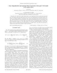
We have performed exact diagonalization calculations
for the symmetric case with t=l.O, V=OS (hence A=O.12),
and U varying from 0 to 4, i.e., from weak coupling to strong
coupling, in the l/2-filled sector. Our results for the ground
state energy per site are shown in Fig. 1. The estimated errors
in extrapolations are within the size of the symbol.
(3)
(4)
(5)
(6)
J. Appl. Phys. 75 (lo), 15 May 1994 0021-8979/94/75(10)/7041/3/$8.00 0 1994 American institute of Physics 7041
Downloaded 14 Jun 2001 to 128.165.156.80. Redistribution subject to AIP license or copyright, see http://ojps.aip.org/japo/japcr.jsp

FIG. 1. The ground state energy per site as function of U for the symmetric FIG. 2. Square of the f orbital local moment as function of U for the same
Anderson lattice model with r=l, V=OS. The dashed line is the weak case as in Fig. 1.
coupling perturbation result from Eq. (7), and the solid line is the strong
coupling perturbation result from Eq. (9). The squares are the exact diagonalixation
results and the uncertainties in the infinite system extrapolation
are within the size of the symbol. 2-1
mfz-2
4u
+JqT (12)
According to perturbation theory,““’ for the symmetric
case in the weak coupling limit where U/A is small, the
ground state energy per site is
with
E(U)=; 2 E;-;
k
-N3
U2
ui=$l+ei/(ei+4V2)1’2] ,
vi=gl-ei/(ei+4V2)“2] .
In the strong coupling limit where U/A is large, the ground
state energy per site is
E(U)=-; +; c e&e,,-? T ;;;:;j 7
k
(10)
with f(ek) being the zero temperature Fermi factor.
We show weak coupling results as the dashed line and
strong coupling results as the solid line in Fig. 1. Note that
there is a singularity in strong coupling limit as ZJ+O
[roughly In(U)] but it is hard to see from Fig. 1.
As U increases from 0 to ~0, electrons tend to localize in
the f orbitals and form local moments. We measure these
moments by m& defined by
4z=((nfT-nf1)2) , (11)
which varies from 1 when U =O, to 1 when U=m.
coupling we have
(7)
(8)
(9)
For weak
while for strong coupling we have
l-f(ek)
m +-q c
k (U/2+ek)’ *
(13)
We show these results as the dashed line and solid line in
Fig. 2, along with data points obtained from our exact diagonalization
studies. Again, estimated errors in extrapolations
are within the size of the symbol.
From Fig. 2, it is evident that weak coupling perturbation
is invalid for U/A>8 and strong coupling perturbation
gives bad answers for U/A

0.2
0
,,,I I I I I I1 I I I I* I I I
0 1
z
3 4
FIG. 3. The ratio of the hybridization matrix element (c!,fi,+hc) to its
lJ=O value as a function of U for the same case as in Fig. 1.
changes between 1 and 2. (3) The Kondo region, in which
one has nf- 1, n,-1. Its range is roughly -U- t