Exact diagonalization and quantum Monte Carlo study of the spin-1 ...

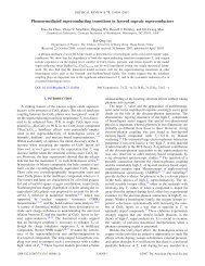
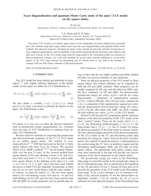
PHYSICAL REVIEW B, VOLUME 64, 214411
Exact diagonalization and quantum Monte Carlo study of the spin- 1 2 XXZ model
on the square lattice
H.-Q. Lin
Department of Physics, Chinese University of Hong Kong, Shatin N.T., Hong Kong
J. S. Flynn and D. D. Betts
Department of Physics, Dalhousie University, Halifax N.S., Canada B3H 3J5
Received 29 March 2001; published 8 November 2001
The spin- 1 2 XXZ model on an infinite square lattice at zero temperature has been studied and is presented
here. Our methods using finite square lattices have been the exact diagonalization and quantum Monte Carlo
methods. The physical properties estimated per lattice vertex include ground-state and first-excited-state energy,
staggered magnetization, and susceptibility in the parallel and perpendicular directions, spin stiffness, and
spin-wave velocity. In the XXZ model range from the Ising model to the Heisenberg model our estimates of
physical properties compare very well with estimates by several other methods published in several other
papers. In the XXZ range between the Heisenberg and XY models there is very little in the literature to
compare with our finite lattice estimates of physical properties.
DOI: 10.1103/PhysRevB.64.214411
I. INTRODUCTION
The XXZ model has been studied and published in many
papers 1–15 with slightly different definitions of the Hamiltonian.
In this paper we define the XXZ Hamiltonian as
HJ x /J x J z
k,l
S k x S l x S k y S l y J z /J x J z
k,l
S k z S l z .
We also define a variable j(J z J x )/(J z J x ), which
proves to be quite convenient in plotting the figures in this
paper. The Hamiltonian is then
1
H 1 j
2
k,l
S k x S l x S k y S l y 1 j
2
k,l
S k z S l z . 2
PACS numbers: 75.10.Hk, 05.50.q, 75.10.Jm
Of course, it is very easy to relate the physical properties
such as ground-state energy, magnetization, etc., estimates
from one type of XXZ Hamiltonian to estimates from another
XXZ Hamiltonian.
We have used two methods of computing the ground-state
and first-excited-state properties of the S1/2 XXZ model
on an infinite square lattice. The method of exact
diagonalization 16–20 ED has been used on the best 12 finite
square lattices with from 18 to 36 vertices. The quantum
Monte Carlo QMC method 21–24,15 has developed substantially
over the past 25 years. In this research method finite
square lattices of the type defining vectors (L,0) and (0,L)
have been used from L6 toL32 inclusive, and in addition,
square lattices of the defining vector pairs (L,L) and
(L,L) for L4, 5, 6, and 7 have also been used. Details
are shown in Table VI in the Appendix. In particular, as there
may be two or more useful lattices with the same number N
of vertices, we label the lattices Ni. The two finite square
lattices 32A with defining vectors 4,4 and (4,4) and 36A
with defining vectors 6,0 and 0,6 have been used for both
ED and QMC for certain properties such as ground-state energy
to show that the now highly sophisticated QMC method
provides very precise estimates of such properties.
There are physical properties of the XXZ model on finite
square lattices that without difficulty can be computed by
both the ED and QMC methods. Other properties can be
readily computed by ED only and still others by QMC only.
We have computed, via ED and QMC, the dimensionless
ground-state energy per vertex, 0 (Ni), and the per vertex
dimensionless z component of magnetization squared,
m z 2 (Ni), without difficulty. Only ED can easily compute the
x or y) component of the magnetization squared per vertex
and the dimensionless first-excited-state energy per vertex,
1 (Ni). On the other hand, only QMC can easily compute
the spin stiffness per vertex, s (Ni), of the XXZ model.
Section II will describe the computation and the statistical
analyses of the physical properties of the XXZ model at the
three ‘‘anchor’’ points. These are the points where J x J z
( j0), the Heisenberg antiferromagnet; J x 0 (j1), the
Ising model; and J z 0(j1), the XY model. Of course,
the physical properties of the Ising model are known exactly.
We have obtained higher precision of the physical properties
of the XXZ model at the XY and Heisenberg points than
anywhere else along the ‘‘ropes’’ between the pairs of anchor
points. Our method of statistical analyses is demonstrated in
this section using the XY ferro or antiferro magnet and the
Heisenberg antiferromagnet QMC and ED data on finite
square lattices. The appropriate finite lattice scaling equations
fitted statistically to the data will provide very precise
estimates of the above properties on the infinite lattice.
The ground-state energy per vertex in the Heisenberg-
Ising range is somewhat similar to the ground-state energy in
the XY-Heisenberg range. This is mentioned at the beginning
of Sec. III and shown in Fig. 3. Section III then goes on to
describe the properties of the XXZ model in the Heisenberg-
Ising range. To fit a curve through a set of estimates at infinity
of any physical property we use the dimensionless independent
variable j. Let us consider the set of p k ()
estimates for some physical property in the Heisenberg-Ising
0163-1829/2001/6421/2144119/$20.00
64 214411-1
©2001 The American Physical Society

H.-Q. LIN, J. S. FLYNN, AND D. D. BETTS PHYSICAL REVIEW B 64 214411
range. A simple function f ( j,) is statistically fitted to the
p k () set of points. The resulting curve and the points can
be displayed in a figure. The properties studied include the
ground-state energy 0 , the staggered magnetization squared
m z 2 , and the parallel susceptibility . Each of the properties
close to the Heisenberg end is very difficult to settle. This is
especially true of the inverse parallel susceptibility.
Section IV compares our T0 infinite N estimates of energy
and staggered magnetization based on finite QMC
and/or ED data with estimates of the same properties obtained
by other colleagues see Refs. 1–4 using methods
such as spin wave, series expansion, CMX, t expansion, etc.
In general, our T0 infinite N estimates of the various properties
of the XXZ model at a number of points along the
Heisenberg-Ising range are closely comparable to most of the
other estimates. However, in most other estimates the finite N
second term coefficient has not been calculated and thus our
second term coefficients have no other estimates with which
to compare.
Section V will first display as an example the finite lattice
data for the physical properties 0 ( j,Ni) and 1 ( j,Ni) for
j1/2. Then analyses similar to that of Sec. III although
with different results are performed. In the XY-Heisenberg
range the physical properties which are finite include the
susceptibility and staggered magnetization squared m x 2 in
the perpendicular spin-space direction, the spin stiffness s ,
and the spin-wave velocity v. Each of them is zero in the
Heisenberg-Ising range. In the XY-Heisenberg range it is
also difficult to settle the properties near the Heisenberg end.
Finally Sec. VI is summary, discussion, and outlook. All
of our large amount of original data remains in our computer’s
memory.
II. SÄ1Õ2 ISING, HEISENBERG, AND XY MODELS,
PROPERTIES AT TÄ0
The Ising, Heisenberg and XY models are special cases of
the XXZ model. The physical properties of the spin- 1 2 Ising
model at zero temperature can easily be calculated exactly.
The physical properties of the S1/2 Heisenberg antiferromagnet
and the XY ferromagnet or antiferromagnet on the
infinite square lattice at T0 have been much studied and
calculated by various methods by many physicists. Nevertheless,
we too have studied these models on the square lattice
at T0 because they are anchor points of the S1/2 XXZ
model. We have used both the exact diagonalization and
quantum Monte Carlo methods to obtain some properties of
these two models on 28 suitable finite bipartite square
lattices. 20 These lattices are listed in Table VI in the Appendix.
For some properties we have used only ED on those
lattices of 18N36 vertices. For other properties we have
used only QMC on lattices of N32.
There is a finite lattice scaling equation for each physical
property of these models. N is the number of vertices of a
finite lattice, and the independent variable in two dimensions
is N 1/2 L 1 . The most extensive and fundamental paper
on finite lattice scaling equations seems to be that by Hasenfratz
and Niedermayer. 25 In particular, for the S1/2 Heisenberg
antiferromagnet the ground-state dimensionless energy
FIG. 1. Ground-state energy per vertex plotted against N 3/2 for
the XY ferromagnet (’s and Heisenberg antiferromagnet (’s.
per vertex, 0 (), is equal to the first-excited-state energy
1 () and in general s (). Furthermore, the next term in
the scaling equation, A HA 3,s , is also independent of s, the S z
state of the Hamiltonian.
Below are some specific scaling equations. For dimensionless
ground-state energies per vertex for the S1/2
Heisenberg antiferromagnet,
HA 0 L HA A HA 3 L 3 A HA 4,0 L 4 •••
and for the S1/2 XY model
XY 0 L XY A XY 3 L 3 A XY 5,0 L 5 •••. 4
The square of the staggered magnetization per vertex,
m 2 x (L), has the same scaling equation for the XY model as
for the Heisenberg model or all points in the XXZ model in
between. Similarly m 2 z (L) has the same scaling equation in
the Heisenberg-Ising range, namely,
m L 2 m 2 B 1 L 1 B 2 L 2 OL 3 .
The next step is to fit statistically the appropriate finite
lattice scaling equation to the set of data under consideration.
We use the statistical programming package S-PLUS from
MathSoft Inc., Seattle, to do the fitting. We have used an
iterative process by throwing out one finite lattice at a time
until all outriders a minority are eliminated.
Figure 1 displays as points the ground-state energy per
vertex of the Heisenberg antiferromagnet, 0 HA (Ni), and of
the XY ferromagnet, 0 XY (Ni), computed on lattices of 18
N1024 vertices. The horizontal variable is L 3 N 3/2 .
Also in Fig. 1 are the two finite lattice scaling equations,
respectively, as two curves fitted statistically to the two sets
of 0 (Ni) data.
3
5
214411-2

EXACT DIAGONALIZATION AND QUANTUM MONTE ... PHYSICAL REVIEW B 64 214411
1 XY L 0 XY L XY L2 XY 1 L 4 D 6 L 6
OL 7 .
Using our ED data we find numerically that
11
and
HA L6.61L 4 9.3L 5 2.9L 6
12
XY L2.37L 4 0.872L 6 . 13
This means that D 5 0 for the XY model.
Next we consider the spin stiffnesses XY s and HA s based
only on QMC data. The relevant finite lattice scaling equations
for the spin stiffness for the HA Ref. 26 and XY Ref.
27 models are
FIG. 2. Ground-state magnetization per vertex plotted against
N 1/2 for the XY ferromagnet (’s and Heisenberg antiferromagnet
(’s.
and
The fitted equations are numerically
0 HA N0.334721.136L 3 0.82L 4
0 XY N0.548820.839L 3 0.30L 5 .
Similarly, Fig. 2 displays as points the ground-state magnetization
squared (m HA x,0 ) 2 (m HA y,0 ) 2 (m HA z,0 ) 2 for the
Heisenberg antiferromagnet and (m XY x,0 ) 2 (m XY y,0 ) 2 for the XY
model. Whereas the (m HA z0
) 2 data are computed via ED and
QMC for the XY model, the (m XY x,0 ) 2 data are computed only
via exact diagonalization, as can be seen in the two sets of
points in Fig. 2. Accordingly the statistically fitted scaling
equation for the Heisenberg antiferromagnet,
m HA z,0 L 2 0.031070.2009L 1 0.196L 2 0.007L 3 ,
8
is more precise than that for the XY model:
m XY x,0 L 2 0.09580.116L 1 0.12L 2 .
The energies of the first excited state, HA 1 () and
XY 1 (), are not by themselves of much interest. This is so
especially since the data leading up to these estimates are
available now only for N36 as the QMC method has not
been used because of serious difficulties. However, according
to Hasenfratz and Neidermayer, 25 1 () 0 () and
also A 3,1 A 3,0 .
Then the susceptibilities HA and XY are obtained 25 from
the equations
and
1 HA L 0 HA L HA L HA 1 L 4 D 5 L 5
D 6 L 6 OL 7
6
7
9
10
and
is
s HA L s HA c 1 L 1 c 3 L 3
s XY L s XY c 3 L 3 .
14
15
The numerical result for the Heisenberg antiferromagnet
s HA L0.08990.015L 1 0.69L 3 .
16
The raw finite lattice data used in the original finite lattice
scaling equation would result in statistical coefficients that
would be two-thirds of the value of the coefficients above
because of the method of obtaining the data. However, this is
not the case for the XY magnet:
s XY L0.26950.49L 3 .
17
It is well known that the spin-wave velocity v is related to
s and via s v 2 . Thus we find v from the s and
data. There is also another way of determining the spin-wave
velocity. Using the second coefficient in the finite lattice
scaling equation for the ground-state or first-excited-state
energy, we obtain another estimate: vA 3 , in which the
geometric square lattice factor 1.437 745.
All these estimates are displayed in Table I. In that table
both the Heisenberg and the XY model data we estimated are
compared to relatively recent estimates by Sandvik 28 and
Sandvik and Hamer. 27 Our estimates of energy and staggered
magnetization agree very closely with those in the recently
published papers. On the other hand, susceptibility and spin
stiffness estimates are not very close to the estimates in the
above-mentioned publication.
Our estimates over a range of j based on QMC and ED
data will be compared with other j range estimates based on
other methods in Sec. IV.
III. ESTIMATED PROPERTIES OF THE XXZ MODEL IN
THE RANGE 0ËjÏ1
The physical properties of the S1/2 XXZ model on the
infinite square lattice are quite different in the two ranges of
j on either side of the antiferromagnetic Heisenberg point, j
0. That is why this paper has two different sections dis-
214411-3

H.-Q. LIN, J. S. FLYNN, AND D. D. BETTS PHYSICAL REVIEW B 64 214411
TABLE I. A comparison of physical properties of the XXZ model on the square lattice at particular,
special points, or anchors. Statistical error of estimation is in parentheses.
Physical
property
Ising
model
Heisenberg antiferromagnet
XY model
Current Sandvik 1997 Current SH 1999
1 0 1/2 0.33472(3) 0.33472(1) 0.54882(3) 0.548824(2)
2
m z 1/4 0.03111 0.031426 0 0
2
m x 0 0.03111 0.031426 0.09582 0.0961
0.1513 0.1252 0.2111 0.20962
s 0 0.0901 0.0881 0.26952 0.26962
v( s /) 1/2 0 0.773 0.822 1.132 1.1342
vA 3 / 0 0.824 0.842 1.204 1.1232
playing the estimates of the properties of the model. The
ground-state or first-excited-state energy per vertex, ( j,),
is more nearly symmetric about the J z J x or j0) point
than any other property we have studied. Therefore we display
( j,) in Fig. 3 over the entire range from the XY
model through the Heisenberg point to the Ising model. In
the range 0 j1, we have used energy scaling law 4. The
( j,) data on the Ising side ( j0) are shown in Table II.
They too are fitted well by the polynomial
j,0.334720.01217j0.34252j 2
0.24204j 3 0.07704j 4 .
18
The ( j,) data on the XY side of the Heisenberg ( j0)
point, shown in Table V, have also been fitted well by the
polynomial
j,0.334720.18205j0.03292j 2 .
19
The lack of symmetry is obvious. Notice that the sum of the
five coefficients in Eq. 19, (1,), is 0.500 07, extremely
close to the exact Ising ground-state energy (1,)
1/2.
Throughout this range the staggered magnetization
squared m x 2 ( j,)0 and the spin stiffness s ( j,)0, although
this is not easy to determine explicitly where 0 j
1. However, m z 2 ( j,)0 and so in Fig. 4 we show a set of
statistically estimated points, m z, j ()m j (), the staggered
magnetization. Furthermore, a curve fitted statistically,
m( j,), using all the points except those two points for j
close to zero, is also in Fig. 4. The simple polynomial equation
fitted to the points is
m j,0.305300.40617j 1/2 0.20935j0.00280j 3/2 .
20
Next we consider , the susceptibility parallel to the spin
space z direction, by examining the scaling equation
1 j,Ni 0 j,Ni j,Ni 1
L 4 D 5 jL 5
D 6 jL 6 OL 7 .
21
TABLE II. Infinite N estimates of several physical properties of
the XXZ model in the range of j from the Ising model ( j1)
toward the Heisenberg antiferromagnet ( j→0). The Heisenberg
data in the last line is obtained directly from Table I.
j 0 () 1 () A 3,0 A 3,1 m z 2 () B 1 1 ()
FIG. 3. The points of 0 () have been estimated statistically
from the precise XXZ data of the finite square lattices. The curves
of ( j,) and ( j,) are derived from polynomials in j.
1 0.5 0 0.25 0 0
9/10 0.4754 0.000 0.2497 0.000 0
4/5 0.4519 0.000 0.2486 0.000 0
5/7 0.4325 0.000 0.2467 0.002 0
3/5 0.4083 0.000 0.2427 0.004 0
1/2 0.3889 0.001 0.2375 0.001 0
7/17 0.3733 0.005 0.2298 0.010 0
1/3 0.3610 0.017 0.2206 0.042 0
3/11 0.3526 0.041 0.2120 0.028 0
1/5 0.3444 0.003 0.1981 0.017 ?
3/23 0.3384 0.009 0.1794 0.023 ?
1/9 0.3371 0.031 NA NA ?
1/11 0.3360 0.047 0.1641 0.059 ?
1/17 NA NA 0.1489 0.092 ?
0 0.33472 1.136 0.03107 0.201 0.151
214411-4

EXACT DIAGONALIZATION AND QUANTUM MONTE ... PHYSICAL REVIEW B 64 214411
FIG. 4. Precisely estimated points m j () in the Heisenberg-
Ising range and a curve m( j,) fitted statistically using all points
labeled with ’s.
For any j1/2 we see very quickly that ( j,Ni)0 except
for the smallest lattices. This can be seen in Fig. 5. In
the intermediate-j region, ( j,Ni)0 only for the larger
lattices. Then at the short range near to the Heisenberg point
we find that ( j,Ni) remains finite even for the largest lattice
available, Ni36A. These three sets of points are also in
Fig. 5. It is clear that the parallel susceptibility is infinite for
1/3 j1. Hence the spin-wave velocity v0.
We can not discover whether in the range 0 j
1/3. To do so we should have the ( j,Ni) for very large
finite square lattices—far beyond the exact diagonalization
and even beyond the quantum Monte Carlo methods in use
now and in the near future. Likely throughout the
whole range 0 j1.
IV. COMPARISON OF PHYSICAL PROPERTIES OF THE
XXZ MODEL AT TÄ0 ESTIMATED BY VARIOUS
METHODS
Many published articles have contained estimates of several
physical properties of the XXZ model on the Ising side
FIG. 5. (N) 0 (N) 1 (N) for the points j1/5 (’s, 1/2
(’s, and 4/5 o’s. (N) is calculated from our finite lattice
ground- and excited-state energy data.
at T0 using a variety of means to do so. The recent paper
by Witte et al. 1 estimated properties of the XXZ model in the
Heisenberg-Ising range using a plaquette expansion. The
properties calculated by them are the ground-state energy,
the staggered magnetization in the z direction in spin space,
and the excited-state gap. For each of these properties their
article displays a table comparing their estimates with estimates
in other papers using five other methods.
In Table III our finite lattice estimates of the ground-state
energy in the range 0 j2/3 are compared with four sets of
other estimates displayed in Ref. 1. Three of these sets were
first published in Refs. 2–4. Note that we use Hamiltonian
2 while a slightly different Hamiltonian has been used in all
the papers referred to in this paragraph. To compare our
0 ( j,), based on the Hamiltonian 2, with that in the paper
by Witte et al., 1 based on their Hamiltonian 22, we first had
to use Eq. 18 to reach the same x points. Second, we had to
multiply simply our data by 2/(1 j) to compare ours with
the data of others.
Our estimate at each of the j points agrees with the aver-
TABLE III. Comparison of our estimates of the XXZ-model ground-state energy 0 ( j,) from Eq. 18
with published estimates by other methods in the range 0 j2/3. All other estimates can be obtained from
Table IV of the paper by Witte et al. Ref. 1 or directly from the papers referred to therein.
x j Finite Plaquette t expansion Third order Series
J x /J z lattice expansion a Laplace b spin wave c expansion d Average
0.2 2/3 0.5068 0.5067 0.5067 0.5066 0.5067 0.5067
0.5 1/3 0.5411 0.5416 0.5416 0.5414 0.5417 0.5415
0.8 1/9 0.6071 0.6069 0.6068 0.6074 0.6069 0.6070
0.9 1/19 0.6365 0.6360 0.6354 0.6367 0.6358 0.6361
0.98 1/99 0.6626 0.6622 0.6609 0.6629 0.6621 0.6621
1.0 0 0.6694 0.6691 0.6677 0.6700 0.6693 0.6691
a Reference 1.
b Reference 2.
c Reference 4.
d Reference 3.
214411-5

H.-Q. LIN, J. S. FLYNN, AND D. D. BETTS PHYSICAL REVIEW B 64 214411
TABLE IV. Comparison of our estimates of the XXZ model staggered magnetization m( j,) with published
estimates by other methods in the range 0 j2/3.
Finite Plaquette t expansion Third order Series
x j lattice expansion a D Padé b CMX b spin wave c expansion d
0.2 2/3 0.4958 0.4955 0.4955 0.4955 0.4957 0.4955
0.5 1/3 0.4695 0.4709 0.4710 0.4710 0.4717 0.4709
0.8 1/9 0.4173 0.4162 0.4173 0.4173 0.4164 0.4169
0.9 1/19 0.3865 0.383 0.386 0.3907 0.3839 0.3855
0.95 1/39 0.3650 0.365 0.36 0.3752 0.3607 0.3627
0.98 1/99 0.3440 0.357 0.35 0.3652 0.3406 0.3422
0.99 1/199 0.3330 0.355 0.34 0.3617 0.3307 0.3319
1.00 0 0.3053 0.353 0.33 0.3582 0.3069 0.307
a Reference 1.
b Reference 2.
c Reference 4.
d Reference 3.
age of the five estimates within a few parts in 10 000. An
important difference between our estimates and the other
four estimates is that the other four methods start from the
exact Ising model or x0 and thus have the least precision
of energy or other properties at x1. In contrast our estimates
for each of several j’s or x’s start at the particular j
with ED and QMC on finite lattices from N18 to very large
vertices. Thence we obtain precise estimates of the energy
or whatever as N→ for any value of j. In particular, for
j0 or x1), the Heisenberg model, we have used energy
data from 28 finite lattices of 18N1024 vertices. We
claim that our estimate 0 (0,)0.66944. As a result the
differences between our estimate at x1 and theirs are as
follows: plaquette, 0.0003; t expansion, 0.0017; spin wave,
0.0006; and series, 0.0001. A similar set of differences can
be seen at x0.99 with the t expansion estimate again the
farthest from the exact diagonalization estimate.
Next we compare our staggered magnetization m with the
estimates from five other methods as displayed in Table V of
Ref. 1. Our estimates are easily derived from Eq. 20.
Notice that throughout the range 0.2x0.9 all six sets
of estimates are quite close to one another. The estimates
would be even closer to each other in the range 0.2x0,
the Ising limit where m()1/2 exactly. In the range 0.90
x0.99 the estimates using plaquette expansion and t expansion
D Padé have larger confidence limits. Our finite lattice
estimates in this range remain closest to the series expansion
estimates and fairly close to the third-order spin
wave estimates. Our estimates of the staggered magnetization
in Table IV are obtained from m( j,) in Eq. 20.
In Table VI of Ref. 1 comparisons are made of five sets of
estimates derived from five methods for the ‘‘excited-state
gap G’’ in the same range as above. The different estimates
of G for the same j diverge greatly as j tends toward j0,
the Heisenberg antiferromagnet. For example, for j1/99
(x0.98) the estimates of G are 0.44, 0.45, 0.52, 0.27, and
0.26. We decided not to bother calculating G in our finite
lattice estimate program.
V. ESTIMATES OF XXZ MODEL PROPERTIES IN THE
RANGE À1ÏjÏ0
Next in Fig. 6 as an example are the ground-state and
first-excited-state ED energy data on all useful finite lattices
of 18N36 vertices in the middle of the XY-Heisenberg
range with j0.5 or J z /J x 1/3. At j1/2 and throughout
the range 1 j0 we have used energy scaling law Eq.
3 rather than Eq. 4. Clearly 1 ( j,) 0 ( j,). Furthermore,
as N 3/2 or L 3 ) reaches zero the two slopes are very
close to equal, A 3,1 (1/2)A 3,0 (1/2).
At this point we introduce the statistical estimates of several
properties of the S1/2 XXZ model on the infinite
square lattice. The range is from the XY model to the
Heisenberg antiferromagnet, i.e., 1 j0. Nonzero properties
in this range that can be calculated include the groundstate
and first-excited-state energies per vertex, 0 () and
1 (), the coefficients of the second term in the energy scal-
FIG. 6. The exact diagonalization energies 0 ( j,Ni) for the
ground state of the XXZ model at j1/2 are shown as ’s and
the 1 ( j,Ni) energies are shown as ’s. The curves are determined
statistically using the finite lattice scaling equation 3.
214411-6

EXACT DIAGONALIZATION AND QUANTUM MONTE ... PHYSICAL REVIEW B 64 214411
TABLE V. Infinite N estimates of several physical properties of
the XXZ model in the range of j from the XY model ( j1) to the
Heisenberg antiferromagnet ( j0).
j 0 () 1 () A 3,0 A 3,1 m x 2 () B 1 s () ()
1 0.54882 0.84 0.095 0.12 0.2695 0.211
9/11 0.50619 0.093 0.12 0.2435 0.207
3/5 0.45714 0.77 0.089 0.13 0.2128 0.203
1/2 0.43445 0.086 0.13 NA 0.200
1/3 0.39888 0.67 0.080 0.14 0.1709 0.195
1/4 0.38099 0.076 0.15 NA 0.191
1/7 0.36010 0.56 0.072 0.14 0.1375 0.181
1/15 0.34586 0.60 0.078 0.00 0.1204 0.152
1/31 0.33985 0.75 0.079 0.10 0.1108 0.124
1/63 0.33725 0.27 NA NA 0.1020 NA
0 0.33472 1.14 0.034 0.18 0.0898 0.151
ing equation, A 3,0 and A 3,1 , the ground-state staggered magnetization
squared in the x direction, m x 2 (), and the coefficient
B 1,0 of the second term in the magnetization scaling
equation, the spin stiffness s , the perpendicular susceptibility
, and the spin-wave velocity v. As the estimated magnetization
on the infinite lattice in the x direction in spin
space has been obtained only from exact diagonalization
data, while the estimated spin stiffness has been obtained
only from the quantum Monte Carlo data, not all the points
in the j range are used for both m x 2 () and s (). These data
are shown in Table V.
The exact diagonalization data used to estimate m x 2 ()
are on the 12 best lattices for which 18N36. We have
estimated m x 2 ( j,) statistically using each set of exact diagonalization
data on finite N for each of ten j’s. These points
are displayed in Fig. 7. Notice that the two points closest to
the Heisenberg j0 point do not follow the trend of the
others. We feel that the scaling, which is based on the
m x 2 ( j,Ni) exact diagonalization data, is more complex in the
FIG. 8. Nine estimated spin stiffness points s, j () in the XY-
Heisenberg range are shown by ’s, and a curve of s ( j,) is fitted
statistically using all points including the j0 Heisenberg point.
range 0.1 j0 than in the range 1.0 j0.1. Accordingly
we do not include the m x 2 (1/7,) and m x
2
(1/15,) data in fitting the coefficients in Eq. 20. Accordingly,
we have not calculated exact diagonalization data
for m x 2 (1/63,Ni). This change can also be seen in Table V
under A 3,0 , m x 2 (), and B 1 in the 0.1 j0 range. To
produce the curve in Fig. 7 the following equation is based
on the seven remaining points:
m x 2 j,0.0500.062 j 1/2 0.017 j.
22
The spin stiffness points s ( j,) over the same range of j
have also been estimated statistically but from the quantum
Monte Carlo finite lattice data only. These s ( j,) points are
shown in Fig. 8. The fitted curve here is determined by the
following equation:
s j,0.09040.0905 j 1/2 0.0878 j.
23
The next property examined in the XY-Heisenberg range
is the perpendicular susceptibility . We have the necessary
data of 0 ( j,Ni) and 1 ( j,Ni), and we use them in Eq.
11 for all sets of 1 j0. The ( j,) is in Table V.
Figure 9 displays these points and the curve determined by
the statistical equation
j,0.14850.1045 j 1/2 0.0430 j. 24
Finally we display the spin-wave velocity v in Fig. 10. It
is well known that v( s / ) 1/2 , and we have s ( j,) and
( j,). Therefore the spin-wave velocity as a function
v( j,) is simply obtained by dividing Eq. 23 by Eq. 24
and then taking the square root of the quotient.
VI. SUMMARY, DISCUSSION, AND OUTLOOK
FIG. 7. Ten precisely estimated magnetization points m 2 x, j () in
the XY-Heisenberg range 1 j0 are shown by ’s, and a curve
of m 2 x ( j,) is fitted statistically using all points with j1/15.
We have studied the spin- 1 2 XXZ model on the infinite
square lattice at zero temperature. To obtain precise data for
our study we have used on finite square lattices the exact
diagonalization and quantum Monte Carlo methods. We used
214411-7

H.-Q. LIN, J. S. FLYNN, AND D. D. BETTS PHYSICAL REVIEW B 64 214411
FIG. 9. Estimated susceptibility points , j () and a curve of
( j,) fitted statistically using all points except 1/15 j
1/31 in the XY-Heisenberg range.
32 finite lattices with 18–1000 vertices. The J z /J x ratios of
the Ising to XY terms we used in the XXZ Hamiltonian were
38. Our data include properties of ground-state and firstexcited-state
energy, staggered magnetization squared in
the two different spin-space directions, (m z 2 ) and (m x 2 ), susceptibilities
and , and finally we calculated data for the
spin stiffness s . Unfortunately we were unable to obtain m x
2
data from the quantum Monte Carlo method or to obtain
spin-stiffness data from the exact diagonalization method.
Any reader will understand that the amount of finite N data
we have computed is far too large to include in the Appendix;
they would require a book.
For each physical property and each j for which we have
data, we have fitted statistically the appropriate scaling equation
for that property and range of j. Even the complete sets
of coefficients of all the scaling equations are too large to
display in one or more appendixes. However, in the special
cases of the Heisenberg model, the XY model, and a few
other values of j we have displayed a few properties in the
text and figures.
We believe that we have obtained for the infinite square
lattice at zero temperature an almost complete set of estimates
of physical properties in one or more of three different
places: the range from the Ising model to near the Heisenberg
antiferromagnet, the range from the XY model to near
the Heisenberg antiferromagnet, and the Heisenberg point
between the two ranges. In the Heisenberg-Ising range, the
range much studied in the past, we have presented in Tables
III and IV our estimates at infinity and those of four or five
other estimates by other methods which are compared with
ours. We have found that our estimates of the energy and
staggered magnetization in this range are as good as the best
of these properties obtained by others.
Our methods using finite lattices—namely, the quantum
Monte Carlo and exact diagonalization methods—are fundamentally
different from familiar methods such as series expansion,
spin wave, plaquette expansion, etc. Each of those
methods in use for the XXZ model start from the exact Ising
model data at T0 and reach as close as possible to the
FIG. 10. The spin-wave velocity points v()
s () 1 () 1/2 in the 1 j0 range. The plotted line is
v( j,).
Heisenberg model with continuously lessening precision, as
can be seen in the tables in Ref. 1 and elsewhere. Our finite
lattice methods do equally well as a function of J x /J z in the
Ising-Heisenberg range except in the area close to the
Heisenberg model where J x J z .
The most important feature of our finite lattice methods is
the ability to study several properties of the XXZ model in
the range from the XY model to close to the Heisenberg
model. In our Sec. V we have displayed in equations and in
Figs. 6–10 such properties as the zero-temperature energy,
perpendicular staggered magnetization and susceptibility,
spin stiffness, and spin-wave velocity. We have not found
estimates by other methods in the XY-Heisenberg range that
we can compare with ours.
In the future we would like to find a way for spin-stiffness
data to be obtained by exact diagonalization on finite lattices
and for perpendicular magnetization data to be obtained by
the quantum Monte Carlo method on finite lattices. We
would like to have a better understanding of the properties of
the XXZ model at zero temperature very close on each side
of the Heisenberg antiferromagnet by obtaining additional
quantum Monte Carlo data on several square lattices considerably
larger than our present 3232 square lattice. Later it
would also be nice to study the XXZ model at finite temperature
and at nonzero magnetic field.
ACKNOWLEDGMENTS
We are very pleased by the large amount of quantum
Monte Carlo data on the XXZ model computed by A. W.
Sandvik and given to us. These data were for the ground
state and first excited state of the energy, the staggered parallel
magnetization, and the spin stiffness on finite square
lattices from N36 to N1024 for several ratios of J z /J x .
He also discussed with us various points in our paper. We
appreciate his help sincerely. We are also pleased at the help
we received from C. J. Hamer in relation to chiral quantum
field theory and W. Blanchard regarding statistical analyses.
214411-8

EXACT DIAGONALIZATION AND QUANTUM MONTE ... PHYSICAL REVIEW B 64 214411
M. Rovers was also very helpful in the initial data analysis
stage. This research has been supported by the Research
Grants Council of Hong Kong, the Natural Science and Engineering
Research Council of Canada, and the Imperial Oil
Charitable Foundation.
TABLE VI. Bipartite finite square lattices used for exact diagonalization
and/or quantum Monte Carlo computation of the properties
of the XXZ model. Each finite bipartite lattice is labeled by its
number of vertices, N, and its place i in the set of those lattices of N
vertices. A pair of vectors L 1 and L 2 define the lattices.
Ni L 1 L 2 Ni L 1 L 2
APPENDIX
In recent papers, 19,20 including this paper, using the
method of exact diagonalization on bipartite finite square
lattices, we examined the quality of the individual finite lattices.
First, we believe that the best bipartite finite square
lattices must have at least eighteen vertices. Second, we have
determined that only the better of the bipartite finite square
lattices of 18–36 vertices should be shown in Table VI below
so that other scientists can use them. An example of a
poor lattice, 24B, sometimes used by others, is defined by
L 1 6,0 and L 2 0,4. Finally, in Table VI the lattices in
the range 50A–1024A are found to be very good. However,
we have not attempted to find more very good lattices within
the latter range.
18A 3,3 (3,3) 72A 6,6 (6,6)
20A 4,2 (2,4) 98A 7,7 (7,7)
22A 2,4 (5,1) 100A 10,0 0,10
24A 4,4 (4,2) 144A 12,0 0,12
24D 1,5 5,1 196A 14,0 0,14
26B 1,5 (5,1) 256A 16,0 0,16
28B 5,3 (1,5) 324A 18,0 0,18
30A 5,3 (5,3) 400A 20,0 0,20
32A 4,4 (4,4) 484A 22,0 0,22
32B 2,6 (4,4) 576A 24,0 0,24
34A 3,5 (5,3) 676A 26,0 0,26
36A 6,0 0,6 784A 28,0 0,28
50A 5,5 (5,5) 900A 30,0 0,30
64A 8,0 0,8 1024A 32,0 0,32
1 N.S. Witte, L.C.L. Hollenberg, and W.H. Zheng, Phys. Rev. B 55,
10 412 1997.
2 Zheng Weihong, J. Oitmaa, and C.J. Hamer, Phys. Rev. B 52, 10
278 1995.
3 Zheng Weihong, J. Oitmaa, and C.J. Hamer, Phys. Rev. B 43,
8321 1991.
4 C.J. Hamer, Zheng Weighong, and P. Arndt, Phys. Rev. B 46,
6276 1992.
5 T. Barnes, D. Kotchan, and E.S. Swanson, Phys. Rev. B 39, 4357
1989.
6 R.R.P. Singh and M.P. Gelfand, Phys. Rev. B 52, 15 695 1995.
7 K. Kubo and T. Kishi, Phys. Rev. Lett. 61, 2585 1988.
8 Y. Okabe and M. Kikuchi, J. Phys. Soc. Jpn. 57, 4351 1988.
9 C.J. DeLeone and G.T. Zimanyi, Phys. Rev. B 49, 1131 1994.
10 R. Bishop, R. Hale, and Y. Xian, Phys. Rev. Lett. 73, 3157
1994.
11 A. Cuccoli, V. Tognetti, and R. Vaia, Phys. Rev. B 52, 10 221
1995.
12 R.F. Bishop, D.J.J. Farnell, and J.B. Parkinson, J. Phys.: Condens.
Matter 8, 11 153 1996.
13 Y. Fukumoto, J. Phys. Soc. Jpn. 65, 569 1996.
14 M. Kohno and M. Takahahi, Phys. Rev. B 56, 3212 1997.
15 A.W. Sandvik, Phys. Rev. B 59, R14 157 1999.
16 J. Oitmaa and D.D. Betts, Can. J. Phys. 56, 897 1978.
17 H.-Q. Lin, Phys. Rev. B 42, 6561 1990.
18 O. Haan, J.-U. Klaetke, and K.-H. Mütter, Phys. Rev. B 46, 5723
1992.
19 D.D. Betts, S. Masui, N. Vats, and G.E. Stewart, Can. J. Phys. 74,
54 1996.
20 D.D. Betts, H.-Q. Lin, and J.S. Flynn, Can. J. Phys. 77, 353
1999.
21 M. Suzuki, Prog. Theor. Phys. 56, 1454 1976.
22 H.G. Evertz, G. Lana, and M. Marca, Phys. Rev. Lett. 58, 86
1987.
23 A.W. Sandvik and J. Kurkijärvi, Phys. Rev. B 43, 5950 1991.
24 A. Sandvik, R.R.P. Singh, and D.K. Campbell, Phys. Rev. B 56,
14 510 1997.
25 P. Hasenfratz and F. Niedermayer, Z. Phys. B: Condens. Matter
92, 911993.
26 T. Einarsson and H.J. Schultz, Phys. Rev. B 51, 6151 1995.
27 A.W. Sandvik and C.J. Hamer, Phys. Rev. B 60, 6588 1999.
28 A.W. Sandvik, Phys. Rev. B 56, 116781997.
214411-9