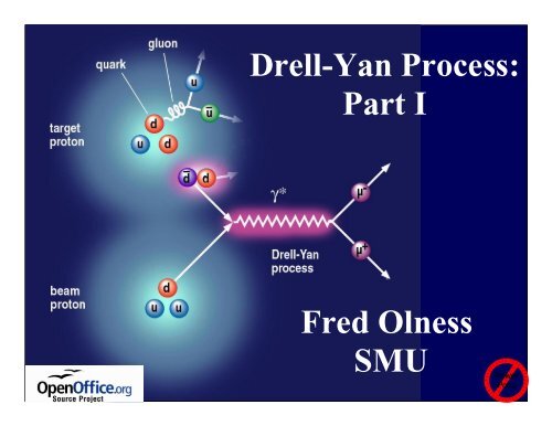
Drell-Yan Process: Part I Fred Olness SMU
Drell-Yan Process: Part I Fred Olness SMU
Drell-Yan Process: Part I Fred Olness SMU

You also want an ePaper? Increase the reach of your titles
YUMPU automatically turns print PDFs into web optimized ePapers that Google loves.
<strong>Drell</strong>-<strong>Yan</strong> <strong>Process</strong>:<br />
<strong>Part</strong> I<br />
<strong>Fred</strong> <strong>Olness</strong><br />
<strong>SMU</strong>
<strong>Part</strong> I: <strong>Drell</strong>-<strong>Yan</strong> <strong>Process</strong><br />
History:<br />
Discovery of J/ψ, Upsilon, W/Z, and “New Physics” ???<br />
Calculation of q q →µ + µ - in the <strong>Part</strong>on Model<br />
Scaling form of the cross section<br />
Rapidity, longitudinal momentum, and x F<br />
Comparison with data:<br />
NLO QCD corrections essential (the K-factor)<br />
σ(pd)/σ(pp) important for d-bar/ubar<br />
W Rapidity Asymmetry important for slope of d/u at large x<br />
Where are we going?<br />
P T<br />
Distribution<br />
W-mass measurement<br />
Resummation of soft gluons
Historical<br />
Background
Our story begins in the late 1960's
Brookhaven National Lab<br />
Alternating Gradient Synchrotron
The Goal:<br />
They found:<br />
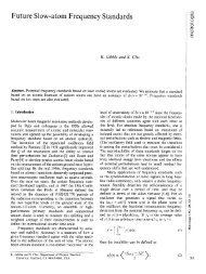
An Early Experiment:<br />
p + N → W + X<br />
p + N → µ + µ − + X<br />
at BNL AGS<br />
Not the W<br />
cross section<br />
M µµ<br />
GeV
What is the explanation???<br />
In DIS, we have two choices for an interpretation:<br />
lepton<br />
current<br />
L µν W µν<br />
interaction<br />
hadron<br />
current<br />
Conserved Current Interactions<br />
The <strong>Part</strong>on Model<br />
What about <strong>Drell</strong>-<strong>Yan</strong>???<br />
? ? ?<br />
The <strong>Part</strong>on Model
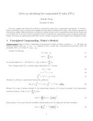
The <strong>Process</strong>: p + Be → e + e - X<br />
Discovery of the J/Psi <strong>Part</strong>icle<br />
very narrow width<br />
⇒ long lifetime<br />
at BNL AGS
q e +<br />
J / ψ<br />
The November Revolution<br />
related by crossing ...<br />
e +<br />
J / ψ<br />
q<br />
q<br />
e -<br />
e -<br />
q<br />
<strong>Drell</strong>-<strong>Yan</strong><br />
Brookhaven AGS<br />
e + e - Production<br />
SLAC SPEAR<br />
Frascati ADONE<br />
R e e hadrons<br />
e e <br />
3<br />
i<br />
Q i<br />
2
More Discoveries with <strong>Drell</strong>-<strong>Yan</strong><br />
1974: The J/Psi (charm) discovery p+N → J/ψ<br />
... 1976 Nobel Prize<br />
1977: The Upsilon (bottom) discovery p+N → ϒ<br />
1983: The W and Z discovery p + p → W/Z<br />
... 1984 Nobel Prize
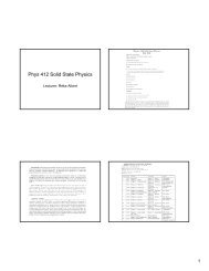
The Future of <strong>Drell</strong>-<strong>Yan</strong><br />
Where do we find<br />
New Physics??<br />
New Higgs Bosons<br />
New W' or Z'<br />
SUSY<br />
... unknown...
Let's<br />
Calculate
First, we'll compute<br />
the partonic σ ^ in the<br />
partonic CMS
Let's compute the Born process:<br />
q q e e <br />
ig <br />
u p 1<br />
q 2 i <br />
u p 3<br />
v p 2<br />
ieQ i ie <br />
v p 4<br />
Gathering factors and contracting g µν , we obtain:<br />
e 2<br />
iMiQ i v p<br />
q 2 2<br />
u p 1<br />
u p 3<br />
<br />
v p 4<br />
Squaring, and averaging over spin and color, ....<br />
M 2 1 2<br />
2<br />
3 1 3<br />
2<br />
Q i<br />
2 e 4<br />
q 4 Tr p 2 p 1<br />
<br />
Tr p 3<br />
<br />
p 4
Let's work out some parton level kinematics<br />
p<br />
p<br />
3<br />
1 θ<br />
p 2<br />
p 4<br />
p 1<br />
s 2<br />
p 2<br />
s 2<br />
1,0,0,1<br />
1,0,0,1<br />
p 3<br />
s 2<br />
1,sin ,0,cos <br />
p 12<br />
p 22<br />
p 32<br />
p 42<br />
0<br />
p 4<br />
s 2<br />
1,sin ,0,cos <br />
Defining the Mandelstam variables ...<br />
s p 1<br />
p 2<br />
2<br />
p 3<br />
p 4<br />
2<br />
t p 1<br />
p 3<br />
2<br />
p 2<br />
p 4<br />
2<br />
u p 1<br />
p 4<br />
2<br />
p 2<br />
p 3<br />
2<br />
t s 2 1cos <br />
u s 2 1cos
We'll now compute the matrix element M<br />
Manipulating the traces, we find ...<br />
Tr p 2<br />
p 1<br />
<br />
Tr p 3<br />
<br />
p 4<br />
<br />
4 p 1<br />
<br />
<br />
p 2<br />
p 2<br />
p 1<br />
g <br />
p 1<br />
p 2<br />
4 p 3<br />
p 4<br />
p 4<br />
p 3<br />
g p 3<br />
p 4<br />
2 5 p 1<br />
p 3<br />
p 2<br />
p 4<br />
p 1<br />
p 4<br />
p 2<br />
p 3<br />
2 3 t 2 u 2<br />
Where we have used:<br />
s2 p 1<br />
p 2<br />
2 p 3<br />
p 4<br />
p 12<br />
p 22<br />
p 32<br />
p 42<br />
0<br />
Putting all the pieces together, we have:<br />
M 2 2 2 2 5 2<br />
Q i <br />
3<br />
t 2 u 2<br />
s 2<br />
with<br />
t 2 p 1<br />
p 3<br />
2 p 2<br />
p 4<br />
u2 p 1<br />
p 4<br />
2 p 2<br />
p 3<br />
q 2 p 1<br />
p 2<br />
2<br />
s<br />
e 2<br />
4
... and put it together to find the cross section<br />
d 1<br />
2 s<br />
M 2<br />
d <br />
In the partonic<br />
CMS system<br />
d <br />
<br />
d 3 p 3<br />
d 3 p 4<br />
2<br />
2 3 2 E 3<br />
2 3 4 p 1<br />
p 2<br />
p 3<br />
p 4<br />
d cos <br />
2 E 4<br />
16 <br />
Recall,<br />
t s<br />
2<br />
1cos and u s<br />
2<br />
so, the differential cross section is ...<br />
d <br />
d cos <br />
and the total cross section is ...<br />
<br />
Q i<br />
2<br />
<br />
2 <br />
6<br />
1<br />
1<br />
s 1<br />
Q 2 2 <br />
i <br />
6<br />
1<br />
s<br />
1cos 2 <br />
1cos <br />
d cos 1cos 2 4 2<br />
9 s<br />
Q i<br />
2<br />
<br />
0
Some Homework:<br />
#1) Show:<br />
d 3 p<br />
d 4 p<br />
2<br />
2 3 2 E 2 4 p 2 m 2<br />
This relation is often useful as the RHS is manifestly Lorentz invariant<br />
#2) Show that the 2-body phase space can be expressed as:<br />
d <br />
<br />
d 3 p 3<br />
d 3 p 4<br />
2<br />
2 3 2 E 3<br />
2 3 4 p 1<br />
p 2<br />
p 3<br />
p 4<br />
d cos <br />
2 E 4<br />
16 <br />
Note, we are working with massless partons, and θ is in the partonic CMS frame
Some More Homework:<br />
#3) Let's work out the general 2→2 kinematics for general masses.<br />
p<br />
p<br />
3<br />
1 θ<br />
p 2<br />
p 4<br />
E 1,2<br />
sm 1<br />
a) Start with the incoming particles.<br />
Show that these can be written in the general form:<br />
p 1<br />
E 1<br />
,0 ,0 ,p p 12<br />
m 1<br />
2<br />
p 2<br />
E 2<br />
,0 ,0 , p p 22<br />
m 2<br />
2<br />
... with the following definitions:<br />
2<br />
m<br />
2<br />
2<br />
2 s<br />
p s,m 2, 2<br />
1<br />
m 2<br />
2 s<br />
a,b,c a 2 b 2 c 2 2 abbcca<br />
Note that ∆(a,b,c) is symmetric with respect to its arguments,<br />
and involves the only invariants of the initial state: s, m 12<br />
, m 22<br />
.<br />
b) Next, compute the general form for the final state particles, p 3<br />
and p 4<br />
. Do this by first<br />
aligning p 3<br />
and p 4<br />
along the z-axis (as p 1<br />
and p 2<br />
are), and then rotate about the y-axis by angle θ.
What does the angular dependence tell us?<br />
Observe, the angular dependence:<br />
q q e e <br />
d <br />
d cos <br />
Q 2 2 <br />
i <br />
6<br />
1<br />
s<br />
1cos 2 <br />
Characteristic of scattering of spin ½ constitutients by a spin 1 vector<br />
q<br />
q<br />
γ<br />
e + e -<br />
Note, for the photon, the mirror image of the above is also valid; hence the symmetric distribution.<br />
The W has V-A couplings, so we'll find: (1+cosθ) 2
Next, we'll compute<br />
the hadronic CMS
Kinematics in the Hadronic Frame<br />
P 1<br />
l +<br />
p 1<br />
= x 1<br />
P 1<br />
P 2<br />
p 2<br />
= x 2<br />
P 2<br />
q=(p 1<br />
+p 2<br />
)<br />
l -<br />
P 1 s 2<br />
P 2 s 2<br />
1,0,0,1<br />
1,0,0,1<br />
P 12 0<br />
P 22 0<br />
s P 1<br />
P 2<br />
2<br />
<br />
s<br />
x 1<br />
x 2<br />
s <br />
Therefore<br />
x 1 x 2 s s Q2<br />
s<br />
Fractional energy 2 between<br />
partonic and hadronic system<br />
d <br />
dQ 2 <br />
q,q<br />
dx 1 dx 2<br />
q x 1<br />
q x 2<br />
q x 1<br />
q x 2<br />
0<br />
Q 2 s<br />
Hadronic<br />
cross<br />
section<br />
<strong>Part</strong>on<br />
distribution<br />
functions<br />
<strong>Part</strong>onic<br />
cross<br />
section
Scaling form of the <strong>Drell</strong>-<strong>Yan</strong> Cross Section<br />
Using:<br />
0<br />
4 2<br />
9 s<br />
Q i<br />
2<br />
and<br />
Q 2 s 1<br />
sx 1<br />
x 2<br />
x 1<br />
we can write the cross section in the scaling form:<br />
Q 4<br />
d <br />
4 2<br />
dQ 2 9<br />
<br />
q,q<br />
1<br />
Q i<br />
2<br />
<br />
dx 1<br />
x 1<br />
q x 1 q x 1 q x 1 q x 1<br />
Notice the RHS is a<br />
function of only τ, not Q.<br />
This quantity should<br />
lie on a universal<br />
scaling curve.<br />
Cf., DIS case,<br />
& scattering of<br />
point-like constituents
Longitudinal Momentum Distributions<br />
<strong>Part</strong>onic CMS has longitudinal momentum w.r.t. the hadron frame<br />
p 12 p 1 p 2 E 12 ,0,0, p L<br />
p 1<br />
= x 1<br />
P 1<br />
p 2<br />
= x 2<br />
P 2<br />
E 12<br />
s 2 x 1 x 2<br />
p 12<br />
p L s 2 x 1 x 2 s 2 x F<br />
x F<br />
is a measure of the longitudinal momentum<br />
The rapidity is defined as:<br />
y 1 2 ln<br />
E 12 p L<br />
E 12<br />
p L<br />
1 2 ln x 1<br />
x 2<br />
dx 1<br />
dx 2<br />
d dy<br />
x 1,2<br />
e y dQ 2 dx F dy d s x F<br />
2<br />
4 <br />
d <br />
dQ 2 dx F<br />
4 2<br />
9Q 4 1<br />
x F<br />
2<br />
4 <br />
<br />
q,q<br />
Q i 2 q x 1<br />
q x 1<br />
q x 1<br />
q x 1
So, we're ready to<br />
compare with data<br />
(or so we think...)
Let's compare data and theory<br />
ÌÐ ½º¾<br />
ÜÔÖÑÒØРùØÓÖ׺<br />
ÜÔÖÑÒØ ÁÒØÖØÓÒ Ñ ÅÓÑÒØÙÑ Ã Ñ׺ <br />
¾ ÃÔ ℄ ÔÈØ ¿¼¼»¼¼ Î ½<br />
Ï¿ ÓÖ ¼℄ ¦ Ï ¿º Î ¾<br />
¿ ËÑ ½℄ ÔÏ ¼¼ Î ½ ¦ ¼¿<br />
´Ô ¹ ÔµÈØ ½¼ Î ¾¿ ¦ ¼<br />
ÔÈØ ¼¼ Î ¿½ ¦ ¼ ¦ ¼¿<br />
Æ¿ ¿℄ ¦ ÈØ ¾¼¼ Î ¾¿ ¦ ¼<br />
ÈØ ½¼ Î ¾ ¦ ¼¿<br />
ÈØ ¾¼ Î ¾¾¾ ¦ ¼¿¿<br />
ƽ¼ Ø ℄ Ï ½ Î ¾ ¦ ¼½¾<br />
¿¾ Ö ℄ Ï ¾¾ Î ¾¼ ¦ ¼¼ ¦ ¼¼<br />
¿ Ò ℄ Ô Ï ½¾ Î ¾ ¦ ¼½¾ ¦ ¼¾¼<br />
½ ÓÒ ℄ Ï ¾¾ Î ½ ¦ ¼¼<br />
J. C. Webb, Measurement of continuum dimuon production in<br />
800-GeV/c proton nucleon collisions, arXiv:hep-ex/0301031.
Oooops,<br />
we need the<br />
QCD corrections<br />
K 1 <br />
2 s<br />
3<br />
2 3<br />
... ...? s<br />
e
Excellent agreement between data and theory<br />
p + Cu at 800 GeV<br />
E605 (p Cu →µ + µ - X) p LAB<br />
= 800 GeV<br />
p + d at 800 GeV<br />
E772 (p d →µ + µ - X) p LAB<br />
= 800 GeV<br />
10 7<br />
M 3 d 2 σ/dx F<br />
dM (nb/GeV 2 /nucleon)<br />
10 10<br />
10 9<br />
10 8<br />
10 7<br />
10 6<br />
10 5<br />
10 4<br />
M 3 d 2 σ/dx F<br />
dM (nb/GeV 2 /nucleon)<br />
10 5<br />
10 3<br />
10<br />
10 -1<br />
10 -3<br />
10 3<br />
10 -5<br />
10 2<br />
10 -7<br />
10<br />
1<br />
10 11 0.2 0.3 0.4 0.5<br />
√τ<br />
pp & pN processes sensitive to<br />
anti-quark distributions<br />
10 -9<br />
10 9 0.08 0.09 0.1 0.2 0.3 0.4<br />
√τ<br />
A. D. Martin, R. G. Roberts, W. J. Stirling and R. S. Thorne,<br />
Eur. Phys. J. C23, 73 (2002);<br />
Eur. Phys. J. C14, 133 (2000);<br />
Eur. Phys. J. C4, 463 (1998)
<strong>Drell</strong>-<strong>Yan</strong> can give us unique and<br />
detailed information about PDF's.<br />
We'll now examine two examples:<br />
1) Ratio of pp/pd cross section<br />
2) W Rapidity Asymmetry
A measurement of d(x)=u(x)<br />
Antiquark asymmetry in the Nucleon Sea<br />
FNAL E866/NuSea<br />
ACU, ANL, FNAL, GSU, IIT, LANL, LSU,<br />
NMSU, UNM, ORNL, TAMU, Valpo.<br />
800 GeV p + p and p + d ! + X<br />
800 GeV<br />
Protons<br />
Counts/0.1 GeV<br />
10 4<br />
10 3<br />
10 2<br />
10<br />
Hadron<br />
Absorber<br />
High Mass<br />
Low Mass<br />
x 10 2<br />
5000<br />
Low Mass<br />
4000<br />
3000<br />
2000<br />
1000<br />
0<br />
2 4 6 8 10 12<br />
10 5 2 4 6 8 10 12 14 16<br />
7500<br />
High Mass<br />
5000<br />
2500<br />
0<br />
2 4 6 8 10 12<br />
d _ / u _<br />
2.2<br />
2<br />
1.8<br />
1.6<br />
1.4<br />
1.2<br />
1<br />
0.8<br />
0.6<br />
Fermilab E866 - <strong>Drell</strong>-<strong>Yan</strong><br />
CTEQ4M<br />
NA 51<br />
MRS(R2)<br />
MRST<br />
±0.032 Systematic error not shown<br />
1<br />
DiMuon Mass (GeV)<br />
0.4<br />
0 0.05 0.1 0.15 0.2 0.25 0.3 0.35<br />
x
Cross section ratio of pp vs. pd<br />
Obtain the neutron PDF via isospin symmetry:<br />
u d<br />
u d<br />
In the limit x 1<br />
>> x 2<br />
:<br />
pp<br />
pn<br />
4 9<br />
u x 1<br />
u x 2<br />
1 9<br />
d x 1<br />
d x 2<br />
4 9<br />
u x 1<br />
d x 2<br />
1 9<br />
d x 1<br />
u x 2<br />
For the ratio we have:<br />
pd<br />
2 pp 1 2<br />
1 1 4<br />
1 1 4<br />
d 1<br />
u 1<br />
1 d 2<br />
1 d 1<br />
d 2<br />
u 2 2<br />
u 1<br />
u 2<br />
1 d 2<br />
u 2<br />
As promised, this provides<br />
information about the<br />
sea-quark distributions<br />
EXERCISE: Verify the above.<br />
pd<br />
2 pp 1 2<br />
1 d 2<br />
u 2
Does the theory match the data???<br />
pd<br />
2 pp 1 2<br />
1 d 2<br />
u 2<br />
2.2<br />
2<br />
Fermilab E866 - <strong>Drell</strong>-<strong>Yan</strong><br />
NA 51<br />
CTEQ4M<br />
σ pd /2σ pp<br />
1.3<br />
1.2<br />
1.1<br />
1<br />
0.9<br />
Fermilab E866 - <strong>Drell</strong>-<strong>Yan</strong><br />
MRS(R2)<br />
CTEQ4M<br />
“CTEQ4M (d _ - u _ = 0)”<br />
d _ / u _<br />
1.8<br />
1.6<br />
1.4<br />
1.2<br />
1<br />
0.8<br />
0.8<br />
1% Systematic error not shown<br />
0.6<br />
±0.032 Systematic error not shown<br />
0.7<br />
0 0.05 0.1 0.15 0.2 0.25 0.3 0.35<br />
Implies R
E866 required significant changes in the hi-x sea distributions<br />
1.3<br />
2.25<br />
1.2<br />
2<br />
1.1<br />
1.75<br />
σ pd /2σ pp<br />
1<br />
0.9<br />
0.8<br />
0.7<br />
0.6<br />
0.5<br />
CTEQ5M<br />
MRST<br />
GRV98<br />
CTEQ5M (d _ = u _ )<br />
0 0.05 0.1 0.15 0.2 0.25 0.3 0.35<br />
x 2<br />
CTEQ4M<br />
MRS(r2)<br />
Less than 1% systematic<br />
uncertainty not shown<br />
d _ /u _<br />
1.5<br />
1.25<br />
1<br />
0.75<br />
0.5<br />
0.25<br />
E866/NuSea<br />
NA51<br />
CTEQ5M<br />
MRST<br />
GRV98<br />
CTEQ4M<br />
MRS(r2)<br />
Systematic Uncertainty<br />
0<br />
0 0.05 0.1 0.15 0.2 0.25 0.3 0.35<br />
x<br />
With increased flexibility in the parameterization of the<br />
sea-quark distributions, good fits are obtained<br />
E.A. Hawker, et al. [FNAL E866/NuSea Collaboration], Measurement of the<br />
light antiquark flavor asymmetry in the nucleon sea, PRL 80, 3715 (1998)<br />
H. L. Lai, et al.} [CTEQ Collaboration], Global<br />
{QCD} analysis of parton structure of the nucleon:<br />
CTEQ5 parton distributions, EPJ C12, 375 (2000)
Next ...<br />
2) W Rapidity Asymmetry
Where do the W's and Z's come from ???<br />
d <br />
dy W 2 3<br />
u(x a<br />
)<br />
proton<br />
u x u x<br />
W + d(x b<br />
)<br />
For anti-proton:<br />
Therefore<br />
G F<br />
2 q q<br />
anti-proton<br />
d x d x<br />
V q q<br />
2<br />
q x a q x b q x b q x a<br />
% of total σ LO<br />
(W + ,W - )<br />
100<br />
10<br />
1<br />
flavour decomposition of W cross sections<br />
W +<br />
W -<br />
_<br />
ud_<br />
du<br />
_<br />
sc _<br />
cs<br />
_<br />
us<br />
_<br />
dc _<br />
su<br />
_<br />
cd<br />
d <br />
dy W 2 3<br />
d <br />
dy W 2 3<br />
G F<br />
2 u x a d x b<br />
G F<br />
2 d x a u x b<br />
0.1<br />
pp<br />
pp<br />
1 10<br />
√s (TeV)<br />
A. D. Martin, R. G. Roberts, W. J. Stirling and R. S. Thorne,<br />
Eur. Phys. J. C23, 73 (2002); Eur. Phys. J. C4, 463 (1998)
A bit of calculation<br />
u(x a<br />
)<br />
proton<br />
anti-proton<br />
W + d(x b<br />
)<br />
A y<br />
<br />
d <br />
dy W d <br />
dy<br />
d <br />
dy W d <br />
dy<br />
W <br />
W <br />
With the previous approximation,<br />
A u x a d x b d x a u x b<br />
u x a d x b d x a u x b<br />
R du x b R du x a<br />
R du x b R du x a<br />
where<br />
R du x d x<br />
u x<br />
We can make Taylor expansions:<br />
x 1,2<br />
x 0<br />
e y x 0<br />
1y<br />
R du x 1,2<br />
R du x 0<br />
yx 0<br />
R' du <br />
EXERCISE: Verify the above.<br />
Thus, the asymmetry is:<br />
A y yx 0<br />
R' du x 0<br />
R du x 0
Unfortunately,<br />
we don't measure the W<br />
directly since W→eν.<br />
Still the lepton contains<br />
important information<br />
Charged Lepton Asymmetry<br />
Charge Asymmetry<br />
0.25<br />
0.2<br />
0.15<br />
0.1<br />
0.05<br />
0<br />
-0.05<br />
-0.1<br />
-0.15<br />
-0.2<br />
CDF 1992-1995 (110 pb -1 e+µ)<br />
CTEQ-3M<br />
RESBOS<br />
MRS-R2 (DYRAD)<br />
MRS-R2 (DYRAD)(d/u Modified)<br />
MRST (DYRAD)<br />
F. Abe, et al. [CDF Collaboration], PRL 81, 5754 (1998)<br />
Measurement of the lepton charge asymmetry in W boson decays<br />
produced in p anti-p collisions,<br />
CTEQ-3M<br />
DYRAD<br />
0 0.5 1 1.5 2<br />
⎮Lepton Rapidity⎮<br />
A y<br />
<br />
d <br />
d<br />
dy l <br />
dy<br />
d d<br />
dy l <br />
dy<br />
l<br />
l<br />
d<br />
u<br />
W -<br />
ν e -<br />
1cos 2
d/u Ratio at High-x<br />
The form of the<br />
d/u ratio at large x<br />
as a function of<br />
1) Parameterization<br />
2) Nuclear Corrections<br />
S. Kuhlmann, et al., Large-x parton distributions, PL B476, 291 (2000)
End of <strong>Part</strong> I: Where have we been???<br />
History:<br />
Discovery of J/ψ, Upsilon, W/Z, and “New Physics” ???<br />
Calculation of q q →µ + µ - in the <strong>Part</strong>on Model<br />
Scaling form of the cross section<br />
Rapidity, longitudinal momentum, and x F<br />
Comparison with data:<br />
NLO QCD corrections essential (the K-factor)<br />
σ(pd)/σ(pp) important for d-bar/ubar<br />
W Rapidity Asymmetry important for slope of d/u at large x<br />
Where are we going?<br />
P T<br />
Distribution<br />
W-mass measurement<br />
Resummation of soft gluons
<strong>Drell</strong>-<strong>Yan</strong> <strong>Process</strong>:<br />
<strong>Part</strong> II<br />
<strong>Fred</strong> <strong>Olness</strong><br />
<strong>SMU</strong>
<strong>Part</strong> II: W Boson Production as an example<br />
Finding the W Boson Mass:<br />
The Jacobian Peak, and the W Boson P T<br />
Multiple Soft Gluon Emissions<br />
Single Hard Gluon Emission<br />
Road map of Resummation<br />
Summing 2 logs per loop: multi-scale problem (Q,q T<br />
)<br />
Correlated Gluon Emission<br />
Non-Perturbative physics at small q T<br />
.<br />
Transverse Mass Distribution:<br />
Improvement over P T<br />
distribution<br />
What can we expect in future?<br />
Tevatron Run II<br />
LHC
Side Note: From pp→γ/Z/W, we can obtain pp→γ/Z/W→l + l -<br />
Schematically:<br />
d q q l l g d q q g d l l <br />
⊗<br />
For example:<br />
d <br />
dQ 2 d t<br />
q q l l g<br />
d <br />
d t<br />
q q g <br />
3 Q 2
<strong>Part</strong> II: W Boson Production as an example<br />
How do we measure the W-boson mass?<br />
u d W e <br />
u<br />
ν<br />
e +<br />
θ<br />
d<br />
<br />
<br />
<br />
Can't measure W directly<br />
Can't measure ν directly<br />
Can't measure longitudinal momentum<br />
We can measure the P T<br />
of the lepton<br />
How can we use this to extract the W-Mass???
u<br />
ν<br />
e +<br />
d<br />
The Jacobian Peak<br />
Suppose lepton distribution is uniform in θ<br />
The dependence is actually (1+cosθ) 2 , but we'll take care of that later<br />
What is the distribution in P T<br />
?<br />
transverse direction<br />
Number of Events<br />
P T<br />
Max<br />
P T<br />
Min<br />
beam direction<br />
We find a peak at P T<br />
max<br />
≈ M W<br />
/2
The Jacobian Peak<br />
Now that we've got the picture, here's the math ... (in the W CMS frame)<br />
p T2 s 4 sin 2 <br />
cos 4 p 2<br />
T<br />
1<br />
s<br />
d cos <br />
dp T<br />
2<br />
2 s<br />
1<br />
cos <br />
So we discover the P T<br />
distribution has a singularity at cosθ=0, or θ=π/2<br />
d <br />
d <br />
d cos <br />
2 2<br />
dp T<br />
d cos dp T<br />
<br />
d <br />
d cos 1<br />
cos <br />
singularity!!!<br />
zero p T<br />
BUT !!!<br />
finite p T<br />
Measuring the Jacobian<br />
peak is complicated if the<br />
W boson has finite P T<br />
.
1) The W-mass is important<br />
fundamental quantity of the<br />
Standard Model<br />
2) P T<br />
Distribution is important<br />
for measuring the W-mass
The W-Mass is an important fundamental quantity<br />
80.360 +/- 0.370<br />
80.410 +/- 0.180<br />
80.470 +/- 0.089<br />
80.433 +/- 0.079<br />
80.350 +/- 0.270<br />
80.498 +/- 0.095<br />
80.482 +/- 0.091<br />
80.452 +/- 0.062<br />
80.427 +/- 0.046<br />
80.436 +/- 0.037<br />
χ 2 /Nexp = 0.4/4<br />
UA2 (W → eν)<br />
CDF(Run 1A, W → eν,µν)<br />
CDF(Run 1B, W → eν,µν)<br />
CDF combined<br />
D0(Run 1A, W → eν)<br />
D0(Run 1B, W → eν)<br />
D0 combined<br />
Hadron Collider Average<br />
LEP II (ee → WW)<br />
World Average<br />
79.5 79.7 79.9 80.1 80.3 80.5 80.7 80.9 81.1 81.3 81.5<br />
Mw (GeV)
The W-Mass is an important fundamental quantity<br />
M W<br />
(GeV/c 2 )<br />
80.6<br />
80.5<br />
80.4<br />
80.3<br />
LEP2<br />
D0<br />
CDF<br />
100<br />
250<br />
500<br />
1000<br />
80.2<br />
80.1<br />
Higgs Mass (GeV/c 2 )<br />
LEP1,SLD,νN data<br />
M W<br />
-M top<br />
contours : 68% CL<br />
130 140 150 160 170 180 190 200<br />
M top<br />
(GeV/c 2 )<br />
T.Affolder, et al. [CDF Collaboration], PRD64, 052001 (2001)<br />
Measurement of the W boson mass with the Collider Detector at Fermilab,
What gives the W<br />
P T ???
What about the intrinsic k T<br />
of the partons?<br />
Assume a Gaussian form:<br />
d 2 <br />
<br />
d 2 0<br />
e p 2<br />
T<br />
p T<br />
k T<br />
760 MeV<br />
problems<br />
good<br />
agreement
For high P T<br />
, we need a hard parton emission<br />
q<br />
q<br />
γ/Z/W<br />
g<br />
R209 at the ISR, 1982<br />
annihilation<br />
q<br />
g<br />
Compton<br />
γ/Z/W<br />
q<br />
Gaussian<br />
e p 2<br />
T<br />
Perturbative<br />
1<br />
p T<br />
2<br />
Combination of Gaussian<br />
& QCD corrections
The complete P T<br />
spectrum for the W boson<br />
Perturbative contributions<br />
+power corrections<br />
The full P T<br />
spectrum<br />
for the W-boson<br />
showing the different<br />
theoretical regions<br />
ÔÔ ´Ï· µ<br />
ÌÉÅ<br />
Perturbative<br />
physics dominates<br />
ÆÓÒÔÖØÙÖØÚ<br />
ÝÒÑ× ´ÒØÖÒ× Ì µ
Road map for<br />
Resummation<br />
⇒<br />
BEFORE<br />
AFTER
NLO P T<br />
distribution for the W boson<br />
q<br />
q<br />
W<br />
g<br />
In the limit P T<br />
→ 0<br />
d <br />
d dy dp T<br />
2 d <br />
d dy<br />
4 s<br />
Born 3<br />
ln s p T<br />
2<br />
p T<br />
2<br />
s<br />
<br />
0<br />
d <br />
d dy dp T<br />
2<br />
dp 2<br />
T <br />
d <br />
d dy<br />
Born<br />
O s<br />
finite<br />
singular<br />
p T<br />
2<br />
<br />
0<br />
d <br />
d dy dp T<br />
2<br />
dp 2<br />
T <br />
d <br />
d dy Born<br />
1<br />
s<br />
p T<br />
2<br />
4 s<br />
3<br />
ln s p T<br />
2<br />
p T<br />
2<br />
dp T<br />
2<br />
<br />
<br />
d <br />
d dy<br />
Parisi & Petronzio, NP B154, 427 (1979)<br />
Dokshitzer, D'yakanov, Troyan, Phy. Rep. 58, 271 (1980)<br />
Born<br />
1 2 s<br />
3 ln 2 s<br />
p T<br />
2<br />
d <br />
d dy Born<br />
exp -2 s<br />
3 ln 2 s<br />
p T<br />
2<br />
effect of gluon<br />
emission<br />
assume this<br />
exponentiates
Resummation of soft gluons: Step #1<br />
Differentiating the previous expression for d 2 σ/dτ dy<br />
Sudakov<br />
Form Factor<br />
d <br />
d dy dp T<br />
2 <br />
d <br />
d dy<br />
4 s<br />
Born 3<br />
ln s p T<br />
2<br />
p T<br />
2<br />
exp 2 s<br />
3 ln 2<br />
We just resummed (exponentiated) an infinite series of soft gluon emissions<br />
Soft gluon emissions<br />
treated as uncorrelated<br />
e s L2 1 s L 2 s L 2 2<br />
2 !<br />
s L 2 3<br />
3!<br />
finite at p T<br />
=0<br />
...<br />
s<br />
p T<br />
2<br />
L ln s p T<br />
2<br />
I've skipped over some details ..<br />
Parisi & Petronzio, NP B154, 427 (1979)<br />
Dokshitzer, D'yakanov, Troyan, Phy. Rep. 58, 271 (1980)<br />
Curci, Greco, Srivastava, PRL 43, 834 (1979); NP B159, 451 (1979)<br />
Jeff Owens, 2000 CTEQ Summer School Lectures
We skipped over a few details ...<br />
1) We summed only the leading logarithmic singularity, α s<br />
L 2 .<br />
We'll need to do better to ensure convergence of perturbation series<br />
2) We assumed exponentiation; proof of this is non-trivial.<br />
The existence of two scales (Q,p T<br />
)≡(Q,q T<br />
) yields 2 logs per loop<br />
3) Gluon emission was assumed to be uncorrelated.<br />
This leads to too strong a suppression at P T<br />
=0.<br />
Will need to impose momentum conservation for P T<br />
.<br />
4) In the limit P T<br />
→ 0, terms of order α S<br />
(µ=P T<br />
) → ∞;<br />
Must handle this Non-Perturbative region.
1) We summed only the leading logarithmic singularity<br />
L ln s p T<br />
2<br />
d <br />
dq T<br />
2<br />
s L<br />
q T<br />
2<br />
1 s 1 L 2 s 2 L 4 ...<br />
s L<br />
q T<br />
2<br />
s 1 L 1 s 2 L 3 s 3 L 5 ...<br />
we resum<br />
these terms<br />
we miss<br />
these terms<br />
d <br />
The terms we are missing are suppressed by α s<br />
L, not α s<br />
!<br />
If (somehow) we could<br />
sum the sub-leading log ...<br />
dq T<br />
2<br />
1 q T<br />
2<br />
1<br />
q T<br />
2<br />
d <br />
dq T<br />
2<br />
s L<br />
q T<br />
2<br />
e s L2 L<br />
s 1 L 1 1 s 2 L 3 L 2 s 3 L 5 L 4 ...<br />
we resum<br />
these terms<br />
we miss<br />
these terms<br />
s 2 L 1 1 s 3 L 3 L 2 s 4 L 5 L 4 ...<br />
Now, the terms we are missing are suppressed only by α s<br />
!
2) We assumed exponentiation; proof is non-trivial<br />
Review where the logs come from<br />
Review one-scale problem (Q)<br />
resummation via RGE<br />
Review two-scale problem (Q,q T<br />
)<br />
resummation via RGE+ Gauge Invariance
Where do the<br />
Logs come from?
Total Cross Section: σ(e + e - ) at 3 Loops<br />
One mass scale: Q 2 . No logarithms!!!
<strong>Drell</strong>y-<strong>Yan</strong> at 2 Loops:<br />
Two mass scales: {Q 2 ,M 2 }. Logarithms!!!
Renormalization Group Equation<br />
More Differential Quantities ⇒ More Mass Scales ⇒ More Logs!!!<br />
d <br />
ln Q2<br />
dQ 2 2<br />
d <br />
ln Q2<br />
and ln q 2<br />
T<br />
dQ 2 2 2<br />
How do we resum logs? Use the Renormalization Group Equation<br />
For a physical observable R:<br />
Using the chain rule:<br />
<br />
dR<br />
d 0<br />
2<br />
<br />
2 2 s 2<br />
2<br />
<br />
s 2 R 2, s 2 0<br />
Solution⇒<br />
s ln Q2<br />
s<br />
Q 2<br />
2 <br />
s<br />
2<br />
<br />
dx<br />
x
Renormalization Group Equation: OVER SIMPLIFIED!<br />
2<br />
<br />
2 s <br />
s 2 R 2, s 2 0<br />
If we expand R in powers of α s<br />
, and we know β,<br />
we then know µ dependence of R.<br />
R ,Q, s 2 R 0<br />
s 2 R 1<br />
ln Q 2 2 c 1<br />
s<br />
2<br />
<br />
2<br />
R 2<br />
ln 2 Q 2 2 ln Q 2 2 c 2<br />
O s<br />
3<br />
<br />
2<br />
Since µ is arbitrary, choose µ=Q.<br />
R Q,Q, s Q 2 R 0<br />
s Q 2 R 1<br />
0c 1<br />
s 2 Q 2 R 2<br />
00c 2<br />
...<br />
We just summed the logs
Two-Scale Problems<br />
For R(µ,Q,α s<br />
), we could resum ln(Q 2 /µ 2 ) by taking Q=µ.<br />
What about R(µ,Q,q T<br />
,α s<br />
); how do we resum ln(Q 2 /µ 2 ) and ln(q T2<br />
/µ 2 ).<br />
Are we stuck? Can't have µ 2 =Q 2 and µ 2 2<br />
=q T<br />
at the same time!<br />
Solution: Use Gauge Invariance; cast in similar form to RGE<br />
Use axial-gauge with axial vector ξ.<br />
This enters the cross section in the form: (ξ•p).<br />
d <br />
d 0<br />
2<br />
d <br />
d 0 p 2 <br />
resum<br />
x, Q2<br />
p 2<br />
2<br />
logs<br />
RGE allows us to vary µ to<br />
2 ,...<br />
Gauge invariance allows us to vary (ξ•p) to resum logs<br />
It is covenient to transform to impact parameter<br />
space (b-space) to implement this mechanism<br />
The details will fill multiple lectures:<br />
See Sterman TASI 1995; Soper CTEQ 1995
d <br />
3) We assumed gluon emission was uncorrelated<br />
d dy dp T<br />
2 ln s p T<br />
2<br />
p T<br />
2<br />
exp 2 s<br />
3 ln 2<br />
s<br />
p T<br />
2<br />
This leads to too strong a suppression at P T<br />
=0.<br />
Need to impose momentum conservation for P T<br />
.<br />
A particle can receive finite k T<br />
kicks,<br />
yet still have P T<br />
=0<br />
k T 4<br />
k T 1<br />
k T 2<br />
k T 3<br />
A convenient way to impose transverse momentum conservation<br />
is in impact parameter space (b-space) via the following relation:<br />
2<br />
n<br />
<br />
i1<br />
k iT p T<br />
<br />
1<br />
2 2 d 2 be i b p T<br />
n<br />
<br />
i1<br />
e i bk iT
4) We encounter Non-Perturbative Physics<br />
S b,Q <br />
Q 2 d 2<br />
1 b 2<br />
A<br />
2 s 2 ln Q2<br />
B<br />
2 s 2<br />
as b →∞, α S<br />
(~1/b) →∞. PROBLEM!!!<br />
Solution: Use a Non-Perturbative Sudakov form factor (S NP<br />
) in the<br />
region of large b (small q T<br />
)<br />
b e S b e S b e S NP b<br />
with<br />
b <br />
<br />
b<br />
1b 2 2<br />
b max<br />
b*<br />
1<br />
0.8<br />
0.6<br />
b max<br />
=1<br />
Note, as b → ∞, b *<br />
→ b max<br />
.<br />
0.4<br />
0.2<br />
0.5 1 1.5 2 b
A Brief (but incomplete) History of Non-Perturbative Corrections<br />
Original CSS:<br />
S CSS NP b h 1<br />
b, a h 2<br />
b, b h 3<br />
b ln Q 2<br />
J. Collins and D. Soper, Nucl.Phys. B193 381 (1981);<br />
erratum: B213 545 (1983); J. Collins, D. Soper, and G. Sterman, Nucl. Phys. B250 199 (1985).<br />
Davies, Webber, and Stirling (DWS):<br />
S DWS NP b b 2 g 1<br />
g 2<br />
ln b max Q 2<br />
C. Davies and W.J. Stirling, Nucl. Phys. B244 337 (1984);<br />
C. Davies, B. Webber, and W.J. Stirling, Nucl. Phys. B256 413 (1985).<br />
Ladinsky and Yuan (LY):<br />
S LY NP b g 1<br />
b bg 3<br />
ln 100 a b g 2<br />
b 2 ln b max Q<br />
G.A. Ladinsky and C.P. Yuan, Phys. Rev. D50 4239 (1994);<br />
F. Landry, R. Brock, G.A. Ladinsky, and C.P.Yuan, Phys. Rev. D63 013004 (2001).<br />
“BLNY”:<br />
S BLNY NP b b 2 g 1<br />
g 1<br />
g 3<br />
ln 100 a b g 2<br />
ln b max Q<br />
F. Landry, “Inclusion of Tevatron Z Data into Global Non-Perturbative QCD Fitting”, Ph.D. Thesis, Michigan State University, 2001.<br />
F. Landry, R. Brock, P. Nadolsky, and C.P.Yuan, PRD67, 073016 (2003)<br />
“q T<br />
resummation”:<br />
F NP q T 1e aq 2<br />
T<br />
(not in b-space)<br />
R.K. Ellis, Sinisa Veseli, Nucl.Phys. B511 (1998) 649-669<br />
R.K. Ellis, D.A. Ross, S. Veseli, Nucl.Phys. B503 (1997) 309-338<br />
Functional Extrapolation:<br />
J. Qui, X. Zhang, PRD63, 114011 (2001); E. Berger, J. Qiu, PRD67, 034023 (2003)<br />
Analytical Continuation:<br />
A. Kulesza, G. Sterman, W. vogelsang, PRD66, 014011 (2002)
Recap: Where have we been???<br />
1) We now summed the two leading logarithmic singularities, α s<br />
(L 2 +L).<br />
2) We still assumed exponentiation; but sketched ingredients of proof.<br />
The existence of two scales (Q,p T<br />
)≡(Q,q T<br />
) yields 2 logs per loop<br />
Use Renormalization Group + Gauge Invariance<br />
Transformation to b-space<br />
3) Gluon emission was assumed to be uncorrelated.<br />
Impose momentum conservation for P T<br />
. (In b-space)<br />
4) Introduced Non-Perturbative function for small q T<br />
(large b) region.
What do we get for the cross section<br />
d <br />
dydQ 2 dq T<br />
2<br />
<br />
<br />
1<br />
<br />
2 2 0<br />
d 2 b e ibqT W b,Q<br />
e S b ,Q S NP b,Q<br />
with<br />
S b,Q <br />
Q 2 d 2<br />
1 b 2<br />
2 A ln Q2<br />
2 B<br />
where we have resummed the soft gluon contributions<br />
I've left out A LOT of material
Putting it all together: σ TOT<br />
= σ RESUM<br />
+σ PERT<br />
-σ ASYM<br />
Let's expand out the resummed expression:<br />
d <br />
s L<br />
e s L2 L<br />
1 2<br />
2<br />
2<br />
dq T q T q T<br />
s L s 2<br />
L 3 L 2 ...<br />
Compare the above with the perturbative and asymptotic results:<br />
d resum s L s 2 L 3 L 2 00 s 3 L 5 L 4 ...<br />
d pert s L s 2 L 3 L 2 L 1 1 s 3 00<br />
d asym s L s 2 L 3 L 2 00 s 3 00<br />
Note that σ ASYM<br />
removes overlap between σ RESUM<br />
and σ PERT<br />
.<br />
We expect:<br />
σ RESUM<br />
is a good representation for q T<br />
~ 0<br />
σ PERT<br />
is a good representation for q T<br />
~ M W
Putting it all together: σ TOT<br />
= σ RESUM<br />
+σ PERT<br />
-σ ASYM<br />
σ TOT<br />
= σ RESUM<br />
+σ PERT<br />
-σ ASYM<br />
TOT<br />
σ RESUM<br />
for q T<br />
~ 0<br />
σ PERT<br />
for q T<br />
~ M W<br />
cross section dσ/dq T<br />
2<br />
RESUM<br />
PERT<br />
ASYM<br />
transverse momentum q T
Putting it all together: σ TOT<br />
= σ RESUM<br />
+σ PERT<br />
-σ ASYM<br />
σ RESUM<br />
for q T<br />
~ 0<br />
Perturbative contributions<br />
+power corrections<br />
TOT<br />
σ PERT<br />
for q T<br />
~ M W<br />
Perturbative<br />
physics dominates<br />
ÔÔ ´Ï· µ<br />
ÌÉÅ<br />
cross section dσ/dq T<br />
2<br />
RESUM<br />
PERT<br />
ASYM<br />
ÆÓÒÔÖØÙÖØÚ<br />
ÝÒÑ× ´ÒØÖÒ× Ì µ<br />
Extra power of q T<br />
dσ/dq T<br />
1<br />
transverse momentum q T<br />
σ TOT<br />
= σ RESUM<br />
+σ PERT<br />
-σ ASYM
Let's compare with some real results<br />
We'll look at Z data where we can measure both leptons for Z→e + e -<br />
different S NP<br />
(b,Q) functions yield difference at small q T<br />
.
Let's return<br />
to the<br />
measurement<br />
of M W
Transverse Mass Distribution<br />
We can measure dσ/dp T<br />
and look for the Jacobian peak.<br />
However, there is another variable that is relatively insensitive to p T<br />
(W).<br />
Transverse Mass<br />
M T 2 e, p eT p T<br />
2<br />
p eT p T<br />
2<br />
Invariant Mass<br />
M 2 e, p e p <br />
2<br />
p e p <br />
2<br />
In the limit of vanishing longitudinal momentum, M T<br />
~ M.<br />
M T<br />
is invariant under longitudinal boosts.<br />
ν<br />
M T<br />
can also be expressed as:<br />
M T 2 e, 2 p eT p T<br />
1cos e <br />
For small values of P TW<br />
, M T<br />
is invariant to leading order.<br />
Exercise:<br />
a) Verify the above definitions of M T<br />
are ≡.<br />
b) For p Te<br />
= +p*+p TW<br />
/2 and p Tν<br />
= -p*+p TW<br />
/2; verify M T<br />
is invariant to leading order in p TW<br />
.<br />
e<br />
∆φ
Compare P T<br />
and Transverse Mass Distribution<br />
zero p T<br />
P T<br />
(GeV)<br />
M T<br />
distribution is<br />
much less sensitive<br />
to P T<br />
of W<br />
finite p T<br />
Still, we need P T<br />
distribution of W to<br />
extract mass and<br />
width with precision<br />
zero p T<br />
finite p T<br />
PDF and p T<br />
(W)<br />
uncertainties will need<br />
to be controlled:<br />
currently uncertainty:<br />
~10-15 & 5-10 MeV/c 2<br />
Statistical precision in Run II<br />
will be miniscule…placing an<br />
enormous burden on control<br />
of modeling uncertainties.
The Future:<br />
Tevatron Run II<br />
... happening now<br />
LHC<br />
... happening soon
Transverse Mass Distribution and M W<br />
Measurement<br />
Transverse Mass<br />
Distribution from CDF<br />
Combined World<br />
Measurements of M W<br />
Events / GeV/c 2<br />
2000<br />
1500<br />
80.360 +/- 0.370<br />
80.410 +/- 0.180<br />
80.470 +/- 0.089<br />
80.433 +/- 0.079<br />
χ 2 /Nexp = 0.4/4<br />
UA2 (W → eν)<br />
CDF(Run 1A, W → eν,µν)<br />
CDF(Run 1B, W → eν,µν)<br />
CDF combined<br />
1000<br />
80.350 +/- 0.270<br />
80.498 +/- 0.095<br />
80.482 +/- 0.091<br />
D0(Run 1A, W → eν)<br />
D0(Run 1B, W → eν)<br />
D0 combined<br />
80.452 +/- 0.062<br />
Hadron Collider Average<br />
500<br />
80.427 +/- 0.046<br />
LEP II (ee → WW)<br />
Fit region<br />
80.436 +/- 0.037<br />
World Average<br />
0<br />
50 60 70 80 90 100 110 120<br />
Transverse Mass (GeV/c 2 )<br />
79.5 79.7 79.9 80.1 80.3 80.5 80.7 80.9 81.1 81.3 81.5<br />
Mw (GeV)<br />
T.Affolder, et al. [CDF Collaboration], PRD64, 052001 (2001)<br />
Measurement of the W boson mass with the Collider Detector at Fermilab,
¡<br />
Preliminary<br />
Run II<br />
measurements<br />
600<br />
500<br />
DO Run2 Preliminary<br />
a)<br />
600<br />
500<br />
b)<br />
400<br />
300<br />
200<br />
100<br />
0<br />
400<br />
300<br />
200<br />
100<br />
0<br />
Events / 2 GeV<br />
100<br />
80<br />
D0 Run II Preliminary<br />
Number of Entries: 604<br />
Peak Mass: 90.8 +- 0.2 GeV<br />
Width: 3.6 +- 0.2 GeV<br />
500<br />
400<br />
25 30 35 40 45 50 55 60 65 70 75<br />
E T<br />
/GeV<br />
300<br />
200<br />
100<br />
0<br />
30 40 50 60 70 80 90 100 110 120<br />
M T /GeV<br />
c)<br />
800<br />
700<br />
600<br />
500<br />
400<br />
300<br />
200<br />
100<br />
0<br />
25 30 35 40 45 50 55 60 65 70 75<br />
E T<br />
/GeV<br />
0 10 20 30 40 50 60<br />
p T<br />
/GeV<br />
d)<br />
60<br />
40<br />
20<br />
0<br />
0 20 40 60 80 100 120<br />
Di-Electron Mass (GeV)
The W-Mass is an important fundamental quantity<br />
M W<br />
(GeV/c 2 )<br />
80.6<br />
80.5<br />
80.4<br />
80.3<br />
LEP2<br />
D0<br />
CDF<br />
100<br />
250<br />
500<br />
1000<br />
80.2<br />
80.1<br />
Higgs Mass (GeV/c 2 )<br />
LEP1,SLD,νN data<br />
M W<br />
-M top<br />
contours : 68% CL<br />
130 140 150 160 170 180 190 200<br />
M top<br />
(GeV/c 2 )<br />
T.Affolder, et al. [CDF Collaboration], PRD64, 052001 (2001)<br />
Measurement of the W boson mass with the Collider Detector at Fermilab,
<strong>Part</strong> II: <strong>Drell</strong>-<strong>Yan</strong> <strong>Process</strong>: Where have we been???<br />
Finding the W Boson Mass:<br />
The Jacobian Peak, and the W Boson P T<br />
Multiple Soft Gluon Emissions<br />
Single Hard Gluon Emission<br />
Road map of Resummation<br />
Summing 2 logs per loop: multi-scale problem (Q,q T<br />
)<br />
Correlated Gluon Emission<br />
Non-Perturbative physics at small q T<br />
.<br />
Transverse Mass Distribution:<br />
Improvement over P T<br />
distribution<br />
What can we expect in future?<br />
Tevatron Run II<br />
LHC
Thanks to ...<br />
Jeff Owens<br />
Chip Brock<br />
C.P. Yuan<br />
Pavel Nadolsky<br />
Randy Scalise<br />
Wu-Ki Tung<br />
Steve Kuhlmann<br />
Dave Soper<br />
and my other CTEQ colleagues<br />
and the many web pages where I borrowed my figures<br />
...
References:<br />
Ellis, Webber, Stirling<br />
Barger & Phillips, 2 nd Edition<br />
Rick Field; Perturbative QCD<br />
CTEQ Handbook<br />
CTEQ Pedagogical Page:<br />
CTEQ Lectures:<br />
C.P. Yuan, 2002<br />
Chip Brock, 2001<br />
Jeff Owens, 2000
Attention:<br />
You have reached the very last page of the internet.<br />
We hope you enjoyed your browsing.<br />
calculate<br />
Now turn off your computer and go out and play.