Chapter 2 Stellar Structure Equations 1 Mass conservation equation
Chapter 2 Stellar Structure Equations 1 Mass conservation equation
Chapter 2 Stellar Structure Equations 1 Mass conservation equation

You also want an ePaper? Increase the reach of your titles
YUMPU automatically turns print PDFs into web optimized ePapers that Google loves.
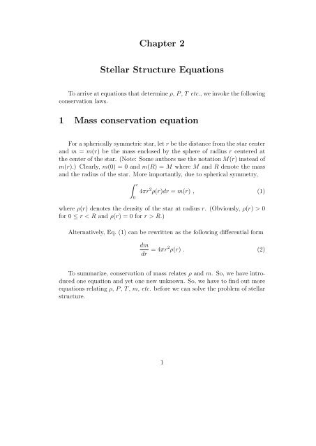
<strong>Chapter</strong> 2<br />
<strong>Stellar</strong> <strong>Structure</strong> <strong>Equations</strong><br />
To arrive at <strong>equation</strong>s that determine ρ, P , T etc., we invoke the following<br />
<strong>conservation</strong> laws.<br />
1 <strong>Mass</strong> <strong>conservation</strong> <strong>equation</strong><br />
For a spherically symmetric star, let r be the distance from the star center<br />
and m = m(r) be the mass enclosed by the sphere of radius r centered at<br />
the center of the star. (Note: Some authors use the notation M(r) instead of<br />
m(r).) Clearly, m(0) = 0 and m(R) = M where M and R denote the mass<br />
and the radius of the star. More importantly, due to spherical symmetry,<br />
∫ r<br />
0<br />
4πr 2 ρ(r)dr = m(r) , (1)<br />
where ρ(r) denotes the density of the star at radius r. (Obviously, ρ(r) > 0<br />
for 0 ≤ r < R and ρ(r) = 0 for r > R.)<br />
Alternatively, Eq. (1) can be rewritten as the following differential form<br />
dm<br />
dr = 4πr2 ρ(r) . (2)<br />
To summarize, <strong>conservation</strong> of mass relates ρ and m. So, we have introduced<br />
one <strong>equation</strong> and yet one new unknown. So, we have to find out more<br />
<strong>equation</strong>s relating ρ, P , T , m, etc. before we can solve the problem of stellar<br />
structure.<br />
1
2 Momentum <strong>conservation</strong> and the <strong>equation</strong><br />
of hydrostatic equilibrium<br />
The next <strong>equation</strong> we introduce comes from the <strong>conservation</strong> of momentum;<br />
or more precisely, in LTE the net force acting on any microscopically<br />
large but macroscopically small region is zero. Inside a star in LTE, the forces<br />
involve are gravity and pressure gradient due to gas or photon. Specifically,<br />
dP<br />
dr = −Gm(r)ρ(r) r 2 . (3)<br />
We denote the central pressure P (0) by P c . And clearly, P (R) can be<br />
approximated by 0.<br />
Eq. (3) can be rewritten as<br />
dP<br />
dm = − Gm<br />
4πr 4 (m) . (4)<br />
Hence,<br />
Since r < R inside the star, we have<br />
P (R) − P (0) =<br />
< −<br />
∫ M<br />
0<br />
∫ M<br />
0<br />
dP<br />
dm dm<br />
Gm<br />
4πR 4 dm<br />
= − GM 2<br />
8πR 4 . (5)<br />
P c > GM 2<br />
8πR 4 (6)<br />
in any star. In particular, this inequality tells us that the central pressure of<br />
our Sun is at least 4.4 × 10 14 dyn/cm 2 ≈ 4 × 10 8 atm.<br />
Multiplying Eq. (4) by the volume V (r) = 4πr 3 /3, we have<br />
∫ P (R)<br />
∫ M<br />
P (0)<br />
V (r)dP = − 1 3<br />
2<br />
0<br />
Gm<br />
r<br />
dm . (7)
Note that the R.H.S. above is Ω/3 where Ω is the gravitational potential<br />
energy of the entire star. Using integration by parts, the L.H.S. above equals<br />
− ∫ V (R)<br />
P dV = − ∫ M<br />
P/ρ dm. Hence, we arrive at<br />
0 0<br />
Ω = −3<br />
∫ M<br />
0<br />
P<br />
ρ<br />
dm . (8)<br />
This <strong>equation</strong> is one form of the virial theorem (sometimes known as the<br />
global form of the virial theorem).<br />
We can use the non-relativistic classical ideal gas to obtain the usual form<br />
of virial theorem. The kinetic energy density of an ideal gas ε is simply given<br />
by ε = N 3<br />
kT and the pressure of an ideal gas is P= N kT= 2 ε. Substituting<br />
V 2 V 3<br />
this relation into above <strong>equation</strong> we get<br />
∫ M<br />
∫<br />
P<br />
V (R) ∫ V (R)<br />
3<br />
0 ρ dm = 3 P dV = 2 εdV = 2U = −Ω (9)<br />
0<br />
Thus, virial theorem tells us that 2U + Ω = 0 where U is the thermal energy<br />
of a star making up of non-relativistic classical ideal gas. Consequently, the<br />
total energy of the star is U + Ω < 0. In other words, the star is in a bound<br />
state.<br />
One consequence of the virial theorem is that upon gravitational contraction,<br />
the star becomes hotter, more tightly bound and have to radiate some<br />
energy to space.<br />
In contrast, if the star is made up of extremely relativistic particles, the<br />
pressure equals one-third the energy density. Hence, in this case, virial theorem<br />
implies that U + Ω = 0. In other words, a star making up of extremely<br />
relativistic particles can be in LTE only when its total energy is 0. So, such<br />
a star is not bounded.<br />
Another consequence of the virial theorem concerns the conversation law.<br />
Consider a star making up of non-relativistic classical ideal gas. Suppose<br />
further that the timescale concerned is small enough that the total energy of<br />
the star is roughly a constant. Since 2U + Ω = 0, the total energy of the star<br />
can be expressed as a function of U (or Ω) alone. Thus, the thermal energy<br />
and the gravitational potential energy of the star are also conserved. In turns<br />
out that this consequence of the virial theorem is useful to understand several<br />
properties of late stage stellar evolution.<br />
3<br />
0
Example. Derive the behavior of m(r),P (r), the luminosity F (r), defined<br />
as dF/dr = 4πr 2 ρq, where q is the energy production rate, and T (r) near<br />
the centre of a star by Taylor expansion for given composition and physical<br />
properties at r = 0: ρ c , P c and T c . The temperature is given by dT/dr =<br />
− (3/4ac) (kρ/T 3 ) (F/4πr 2 ), where k is the opacity and a is the radiation<br />
constant.<br />
If we adopt r as independent space variable, the Taylor expansion near<br />
r = 0 for any function f(r) is<br />
f = f c +<br />
( ) df<br />
r + 1 dr<br />
c<br />
2<br />
( d 2 f<br />
r<br />
dr<br />
)c 2 + 1 ( ) d 3 f<br />
r 3 + ..., (10)<br />
2 6 dr 3<br />
and we retain only the first non-vanishing term besides f c . For the mass<br />
m(r) we have m c = 0 (boundary condition), and from the mass continuity<br />
<strong>equation</strong> we have<br />
( d 3 m<br />
( d 2 m<br />
dr 3 )c<br />
( ) dm<br />
= 4π ( r 2 ρ ) = 0, (11)<br />
dr<br />
c<br />
c<br />
dr 2 )c<br />
(<br />
= 4π 2rρ + r 2 dρ )<br />
= 0, (12)<br />
dr<br />
c<br />
(<br />
= 4π 2ρ + 4r dρ<br />
dr + d2 ρ<br />
r2 = 8πρ<br />
dr<br />
)c<br />
2 c . (13)<br />
Therefore near the centre<br />
m(r) = 4 3 πρ cr 3 , (14)<br />
as if the density were uniform and equal to the central value. For the pressure<br />
P (r) we have<br />
( ) dP<br />
(<br />
= − ρ gm ( ) 4πGρ<br />
= −<br />
dr<br />
c<br />
r<br />
)c<br />
2 r<br />
= 0, (15)<br />
2 3<br />
c<br />
4
( d 2 P<br />
dr 2 )c<br />
= −<br />
( dρ Gm<br />
+ ρ G dm<br />
dr r 2 r 2 dr − 2ρGm r<br />
)c<br />
3<br />
= − 4πGρ2 c<br />
, (16)<br />
3<br />
Therefore near the centre<br />
P (r) = P c − 2 3 πGρ2 cr 2 . (17)<br />
For the luminosity F (r) we have F c = 0 (boundary condition), and<br />
( d 2 F<br />
dr 2 )c<br />
( ) dF<br />
= 4π ( r 2 ρq ) = 0, (18)<br />
dr<br />
c<br />
c<br />
(<br />
= 4π 2rρq + r 2 dρ<br />
dr q + r2 ρ dq )<br />
= 0, (19)<br />
dr<br />
c<br />
( d 3 F<br />
dr 3 )c<br />
= 4π [ 2ρq + r (...) + r 2 (..) ] c = 8πρ cq c . (20)<br />
Therefore near the centre<br />
F (r) = 4 3 πρ cq c r 3 . (21)<br />
For the temperature T (r) we obtain<br />
( ) dT<br />
= − 3 ( kρ F<br />
= −<br />
dr<br />
c<br />
16πac T 3 r<br />
)c<br />
1 ( ) kρ 2 q<br />
2 4ac T r = 0, (22)<br />
3<br />
( d 2 T<br />
dr 2 )c<br />
= − 3 [ ( )<br />
kρ d F<br />
+ F (<br />
d kρ<br />
= −<br />
16πac T 3 dr r 2 r 2 dr T<br />
)]c<br />
1<br />
3 4ac<br />
k c ρ 2 cq c<br />
. (23)<br />
Tc<br />
3<br />
5
Therefore near the centre<br />
T (r) = T c − 1<br />
8ac<br />
k c ρ 2 cq c<br />
r 2 . (24)<br />
Tc<br />
3<br />
Note that these relations hold regardless of the functional dependence<br />
P (ρ, T ), q (ρ, T ), and k (ρ, T ).<br />
3 Simple stellar models<br />
So far, we have 3 unknowns, namely, m(r), ρ(r) and P (r) but only two<br />
<strong>equation</strong>s, namely, the mass <strong>conservation</strong> <strong>equation</strong> and <strong>equation</strong> of hydrostatic<br />
equilibrium. So, we need another <strong>equation</strong> to relate m, ρ and P .<br />
Astronomers have proposed a number of extremely simplified <strong>equation</strong>s to<br />
fulfill this task. Since all these proposed <strong>equation</strong>s are not derived from first<br />
principle, they are nothing more than crude approximations of the realistic<br />
situation. Yet, these approximations are sometimes quite useful to investigate<br />
the approximate structure of a star.<br />
The first such model is called constant density model, namely, we assume<br />
ρ is a constant inside the entire star. The second one is called the linear<br />
density model, namely, ρ(r) = ρ c (1 − r/R) where ρ c is a constant. You may<br />
solve m(r) and P (r) in the above two models yourself.<br />
4 The polytrope model<br />
The last such model I am going to introduce, which is the most important<br />
model of this kind, is called the polytrope model. We assume that<br />
P = Kρ γ (25)<br />
for some constants K and γ. Note that this model is based on the observation<br />
that P and ρ follow the above <strong>equation</strong> for ideal gas in various situations such<br />
6
as adiabatic expansion. With this in mind, we expect that γ varies from 4/3<br />
to 5/3.<br />
Combining the mass <strong>conservation</strong> and hydrostatic equilibrium <strong>equation</strong>s,<br />
we have<br />
( )<br />
1 d r<br />
2<br />
dP<br />
= −4Gπρ . (26)<br />
r 2 dr ρ dr<br />
Write γ = 1 + 1/n, then the above <strong>equation</strong> can be written as<br />
[<br />
]<br />
(n + 1)K d<br />
r 2 (1−n)/n dρ<br />
ρ = −ρ . (27)<br />
4πGnr 2 dr<br />
dr<br />
The boundary conditions for this differential <strong>equation</strong>s are ρ(R) = 0 and<br />
dρ(0)/dr = 0. (Do you know why?)<br />
Let ρ = ρ c θ n where ρ c is the central density of the star, we have<br />
(<br />
1 d<br />
ξ 2 dθ )<br />
= −θ n , (28)<br />
ξ 2 dξ dξ<br />
where r = [(n + 1)Kρ (1−n)/n<br />
c /4πG] 1/2 ξ. The corresponding boundary conditions<br />
are θ = 1 and dθ/dξ = 0 at ξ = 0. This <strong>equation</strong> is called Lane-Emden<br />
<strong>equation</strong> and can be solved numerically.<br />
The significance of the polytrope model is that Lane-Emden <strong>equation</strong> is<br />
independent of the mass M, radius R and central density ρ c of a star. So,<br />
once you have numerically solved the Lane-Emden <strong>equation</strong> for a given value<br />
of n, the numerical solution can be used to deduce the solution of any star<br />
with the same polytropic index n (or γ).<br />
For the special cases of n = 0, n = 1 and n = 5, Lane-Emden <strong>equation</strong><br />
can be solved exactly. The case of n = 0 is easy. You may work out by<br />
yourself that θ(ξ) = 1 − ξ 2 /6; and hence<br />
ρ = ρ c whenever ξ ≠ √ 6 . (29)<br />
The case of n = 1, Lane-Emden <strong>equation</strong> can be rewritten as<br />
d 2<br />
(ξθ) = −ξθ (30)<br />
dξ2 7
whose solution that matches the correct boundary conditions above is θ(ξ) =<br />
sin ξ/ξ. Hence,<br />
ρ = ρ c<br />
sin ξ<br />
ξ<br />
. (31)<br />
For the case of n = 5, Lane-Emden <strong>equation</strong> can be rewritten as<br />
d 2 z<br />
dt = z(1 − z4 )<br />
2 4<br />
, (32)<br />
where ξ = e −t and θ = z/(2ξ) 1/2 . Multiplying Eq. (32) by dz/dt, we obtain<br />
1<br />
2<br />
( ) 2 dz<br />
= 1 dt 8 z2 − 1 24 z6 + C . (33)<br />
Boundary conditions demand that C = 0 and hence<br />
dz<br />
dt = −z 2<br />
) 1/2 (1 − z4<br />
. (34)<br />
3<br />
After making the substitution z 4 /3 = sin 2 ζ and upon integration, we have<br />
e −t = C ′ tan(ζ/2) where C ′ is a constant of integration. Applying the boundary<br />
conditions and after simplification, we obtain<br />
( ) −5/2<br />
ρ = ρ c 1 + ξ2<br />
. (35)<br />
3<br />
(Could you express ρ c as a function of M and R? Besides, could you<br />
express ρ and P as a function of r?)<br />
It is straight-forward to check that the smallest positive root for the<br />
solution θ(ξ) of the Lane-Emden <strong>equation</strong> equals ξ = ξ 1 ≡ √ 6 and ξ = ξ 1 ≡ π<br />
when n = 0 and 1 respectively. This value of ξ 1 corresponds to the boundary<br />
of a star. On the other hand, θ ≠ 0 for any real-valued ξ for n = 5. In<br />
other words, the solution of the Lane-Emden <strong>equation</strong> for n = 5 does not<br />
correspond to a physical star. In fact only n < 5 and n ≠ 1 can correspond<br />
to a physical star (cf. table 1 in supplementary notes).<br />
8
By substituting θ and ξ in the Lane-Emden <strong>equation</strong> back our <strong>equation</strong> of<br />
mass <strong>conservation</strong> (also known as <strong>equation</strong> of (mass) continuity) and <strong>equation</strong><br />
of hydrostatic equilibrium, we obtain<br />
[ ] 1/2 (n + 1)K<br />
R =<br />
ρ (1−n)/2n<br />
c ξ 1 , (36)<br />
4πG<br />
where ξ 1 is the smallest positive value of ξ having θ(ξ) = 0,<br />
[ ] 3/2 (n + 1)K<br />
M = 4π<br />
ρ (3−n)/2n<br />
c<br />
4πG<br />
[<br />
−ξ 2 dθ ]∣<br />
∣∣∣ξ=ξ1<br />
, (37)<br />
dξ<br />
and<br />
[<br />
P c = GM ( ) ] ∣ 2<br />
2 −1∣∣∣∣∣ξ=ξ1 dθ<br />
4π(n + 1)<br />
, (38)<br />
R 4 dξ<br />
¯ρ =<br />
M [<br />
4πR 3 /3 = ρ c − 3 ]∣<br />
dθ ∣∣∣ξ=ξ1<br />
, (39)<br />
ξ dξ<br />
Ω = − 3 GM 2<br />
5 − n R . (40)<br />
Note that R is independent of ρ c for n = 1, Ω > 0 for n > 5, Ω is<br />
undefined for n = 5. Therefore, the polytropic models for n = 1 and n ≥ 5<br />
are not physical. (Can you verify that M is finite, P c is infinite and ¯ρ is 0<br />
for case of n = 5?)<br />
Interestingly, for n = 3, the mass of the star is independent of its central<br />
density. This particular polytropic index is sometimes also called the Eddington<br />
standard model. (We shall say more about the Eddington standard<br />
model later in the next chapter.)<br />
Example. For a given mass M and central pressure P c , which polytrope<br />
yields a bigger star: that of index 1.5 or that of index 3?<br />
The central pressure of the star can be written as<br />
P c = (4π) 1/3 B n GM 2/3 ρ 4/3<br />
c . (41)<br />
9
(Remark : You can check above <strong>equation</strong> yourself and B n contains all n-<br />
dependent coefficients. In table 2 of Supplementary notes, you can see that<br />
B n varies very slowly with n. )<br />
For a given M and P c we obtain<br />
( ) 3/4<br />
ρ c,1.5 B3<br />
= . (42)<br />
ρ c,3 B 1.5<br />
The central density of the polytropic star is given in terms of the mean<br />
density as<br />
M<br />
ρ c = D n ¯ρ = D n<br />
4πR 3 /3 , (43)<br />
where<br />
[ ( ) ] −1<br />
3 dθ<br />
D n = −<br />
, (44)<br />
ξ 1 dξ<br />
ξ 1<br />
are some constants. For a given M we obtain the ratio of radii R(n) as<br />
R (1.5)<br />
R (3)<br />
=<br />
=<br />
(<br />
D1.5<br />
(<br />
D1.5<br />
) 1/3 ) 1/3 ( ) 1/4<br />
ρ c,3<br />
B1.5<br />
=<br />
D 3 ρ c,1.5 D 3 B 3<br />
( ) 1/3 ( ) 1/4 5.991 0.206<br />
< 1, (45)<br />
54.81 0.157<br />
and therefore<br />
R(3) > R (1.5) . (46)<br />
This result makes sense because for a large polytropic index, the star is stiffer<br />
and hence its pressure can resist a bigger gravity so the star should be larger<br />
for the same mass.<br />
Example. Capella is a binary star discovered in 1899, with a known<br />
orbital period, which enables the determination of the mass and radius of the<br />
10
ighter component: M = 8.30 × 10 33 g and R = 9.55 × 10 11 cm. Assuming<br />
that the star can be described by a polytrope of index 3, find the central<br />
pressure and the central density. Check wether the central pressure satisfies<br />
the inequality P c > GM 2 /8πR 4 .<br />
The central density is given by<br />
M<br />
ρ c = D n ¯ρ = D n<br />
4πR 3 /3 , (47)<br />
and we obtain ρ c = 1.2 × 10 −1 g/cm 3 . In order to obtain the central pressure<br />
as a function of M and R we eliminate ρ c between the above <strong>equation</strong> and<br />
thus obtaining<br />
P c = (4π) 1/3 B n GM 2/3 ρ 4/3<br />
c , (48)<br />
P c = GM 2<br />
4πR 4 [<br />
(3D n ) 4/3 B n<br />
]<br />
. (49)<br />
The term in square brackets exceeds unity for all n and hence<br />
P c > GM 2<br />
4πR 4 > GM 2<br />
8πR 4 . (50)<br />
Thus the inequality is generally satisfied by polytropic models. For Capella,<br />
with n = 3, P c = 6.1 × 10 13 dyn/cm 2 .<br />
5 Energy <strong>conservation</strong> and the energy production<br />
<strong>equation</strong><br />
Now, we want to go further than simple stellar models.<br />
introducing a few more <strong>equation</strong>s.<br />
We do so by<br />
11
With our LTE assumption, matter in the star is in thermal equilibrium.<br />
Thus, the gas inside a star will not expand or contract; the work done by the<br />
gas is zero. Let L(r) denotes the luminosity at the spherical shell with radius<br />
r centered at the core of the star. (That is, L(r) is the energy per unit time<br />
moves out of the spherical shell of radius r.) Energy <strong>conservation</strong> demands<br />
that<br />
dL<br />
dr = 4πr2 ρ(r)ϵ(r) , (51)<br />
where ϵ is the rate of energy production per unit mass of material at the<br />
radius r from the stellar center. Note that ϵ is an implicit function of density<br />
ρ, temperature T and chemical composition. (Note: a few authors use the<br />
notation q instead of ϵ.)<br />
Using Eq. (2), the above energy production <strong>equation</strong> can be written as<br />
dL<br />
dm<br />
= ϵ(r) . (52)<br />
Note that L(0) = 0 and L(R) = L where L is the luminosity of the star.<br />
Besides, the region with ϵ(r) > 0 is the region where nuclear fusion takes<br />
place.<br />
6 Some important timescales<br />
• The free-fall / dynamical timescale: For a star with mass M and<br />
radius R, the escape velocity or free fall velocity is of order of √ GM/R.<br />
The free-fall timescale is, therefore, of the order of τ ff ≈ R/ √ GM/R =<br />
√<br />
R3 /GM ≈ 1/ √ G¯ρ where ¯ρ denotes the mean density of the star.<br />
For our Sun, the free-fall timescale is of order of an hour. In short, any<br />
force that is unbalanced inside a star occurs at the free-fall timescale.<br />
Thus, if we are interested in the processes of a stable star over a time<br />
span which is much longer than the free-fall timescale, then we are safe<br />
to assume that the star is in mechanical equilibrium.<br />
• The Kelvin-Helmholtz timescale: This is the timescale τ KH for a<br />
star to radiate its thermal energy away at constant luminosity. By<br />
virial theorem,i.e. KE=PE/2 or KE (the thermal energy) ∼ GM 2 /R,<br />
therefore τ KH ≈ GM 2 /RL. For our Sun, τ KH is about 3 × 10 7 yr. For a<br />
time much longer than the Kelvin-Helmholtz timescale, we may safely<br />
assume that the star is in thermal equilibrium.<br />
12
• The nuclear burning timescale: This is the timescale for burning<br />
all the nuclear fuel of a star at constant luminosity and is therefore<br />
equal to τ nucl ≈ Mc 2 ∆/L, where ∆ ≈ 10 −3 is the typical binding<br />
energy of a nucleon divided by the rest energy of the nucleon. For our<br />
Sun, τ nucl ≈ 10 11 yr. The nuclear burning timescale is a rough estimate<br />
of the lifespan of a star. (You may notice that the nuclear burning<br />
timescale overestimates the lifespan of a star. Do you know why?)<br />
Since τ ff ≪ τ KH ≪ τ nucl , we know once again that our assumption<br />
of LTE is a good approximation to study the interior structure and<br />
evolution of a star.<br />
7 Equation of state<br />
So far, we have used the <strong>conservation</strong> of mass, energy and momentum<br />
to construct three <strong>equation</strong>s for stellar structure. Yet, we have P , T , m, ρ,<br />
L, ϵ, as well as the chemical composition as a function of r for variables.<br />
To further our analysis, we have to look for <strong>equation</strong>s that tell us specific<br />
properties of the material in a star. One such <strong>equation</strong> is the <strong>equation</strong> of<br />
state (EOS), namely, an <strong>equation</strong> expressing the pressure P as a function of<br />
T , ρ and chemical compositions.<br />
To model a star, astrophysicists may use some extremely accurate and<br />
hence complicated EOSs. I shall not do so in this introductory course for the<br />
following reason. Although those EOSs more accurately model the material<br />
behavior, their predictions on the interior structure of a star are in most cases<br />
not significantly different from the simple EOS we will use in this course. The<br />
simplest EOS, which at the same time turns out to be the one we will use in<br />
this course, is the ideal gas law that you have learned in high school. That<br />
is, P = nkT where n is the number density of gas particle.<br />
Ideal gas law is a good approximation to describe the properties of matter<br />
in a star. To see why, I first have to introduce the Saha <strong>equation</strong> discovered<br />
by M. Saha in 1920.<br />
13
7.1 Derivation of Saha Equation<br />
Recall from the course Statistical Mechanics and Thermodynamics that<br />
for a particle (or system of particles), the probability of a particle is in state<br />
s is proportional to g s e −E s/kT where g s is the degeneracy of state s and E s is<br />
the energy of state s relative to some fixed reference energy level (sometimes<br />
taken to be the ground state). More importantly, the proportionality constant<br />
is the same for all the states. Thus, the ratio of the probability that<br />
the particle is in state (s + 1) to the probability that it is in state s is given<br />
by the Boltzmann formula<br />
g s+1<br />
g s<br />
e −(E s+1−E s)/kT . (53)<br />
The Statistical Mechanics and Thermodynamics course also tells us that the<br />
thermodynamic properties of a system with fixed number of particles N and<br />
fixed temperature T and fixed volume V is encoded in the so-called partition<br />
function<br />
Z ≡ ∑ ( ) −Ei<br />
g i exp , (54)<br />
kT<br />
i<br />
where the sum is over all possible energy states of the system. Furthermore,<br />
the ratio between the mean number of particles N s in state s and the total<br />
number of particles N ≡ ∑ N j in a sample is given by<br />
N s<br />
N =<br />
g se −E s/kT<br />
∑<br />
j g je −E j/kT<br />
≡ g se −E s/kT<br />
Z<br />
. (55)<br />
For an ideal classical non-relativistic gas particle with ground state energy<br />
E 0 and degeneracy g, its partition function is given by<br />
∫ ∫<br />
g<br />
Z(1, V, T ) =<br />
e −(E 0+p 2 /2m)/kT d 3 ⃗x d 3 ⃗p<br />
(2π) 3<br />
=<br />
gV<br />
(2π) 3 e−E 0/kT<br />
= gV<br />
λ 3 e−E 0/kT<br />
∫ +∞<br />
0<br />
4πp 2 e −p2 /2mkT dp<br />
(56)<br />
where m is the mass of the particle and<br />
√<br />
2π<br />
λ ≡ <br />
mkT . (57)<br />
14
Note that we have assumed that the momentum of the gas particle is isotropically<br />
distributed in order to obtain the above expression for Z(1, V, T ). The<br />
partition function of a system of N indistinguishable classical non-relativistic<br />
ideal gas particles each with ground state energy E 0 and degeneracy g is then<br />
given by<br />
Z(1, V, T )N<br />
Z(N, V, T ) = . (58)<br />
N!<br />
Recall again from the Statistical Mechanics and Thermodynamics course<br />
that the most convenient method to study the situation in which the particle<br />
number in the system may change is to use the so-called grand partition<br />
function<br />
+∞∑<br />
( ) µN<br />
Q(µ, V, T ) ≡ Z(N, V, T ) exp , (59)<br />
kT<br />
N=0<br />
where µ is the chemical potential. In the thermodynamic limit, µ can be<br />
interpreted as the work needed to add one extra particle to the system at<br />
constant V and T . The grand partition function encodes the thermodynamical<br />
information of a system with fixed chemical potential, volume and<br />
temperature. For N → ∞, <strong>equation</strong> (59) can be evaluated exactly as<br />
[ ]<br />
gV<br />
Q(µ, V, T ) = exp<br />
λ 3 e(µ−E 0)/kT<br />
. (60)<br />
You can refer to the detail of any standard Statistical Mechanics and Thermodynamics<br />
textbook for detail.<br />
More generally, the grand partition function of a system of interacting<br />
particles of various different species such that each species can be approximated<br />
by a classical non-relativistic ideal gas is given by<br />
Q({µ s }, V, T ) ≡ ∏ s<br />
Q(µ s , V, T ) = exp<br />
[ ∑<br />
s<br />
g s V<br />
λ 3 s<br />
e (µ s−E 0,s )/kT<br />
]<br />
, (61)<br />
where the s is the species label. Hence, the corresponding grand potential<br />
equals<br />
G({µ s }, V, T ) ≡ −kT ln Q = −kT ∑ ( )<br />
g s V µs − E 0,s<br />
exp<br />
. (62)<br />
λ 3 s s kT<br />
15
Note<br />
∑<br />
that G is minimized in chemical equilibrium. Since G = E − T S −<br />
s µ sN s , we have<br />
N s = − ∂G<br />
∂µ s<br />
∣<br />
∣∣∣T,V,{µi<br />
} i≠s<br />
= g sV<br />
λ 3 s<br />
( )<br />
µs − E 0,s<br />
exp<br />
. (63)<br />
kT<br />
By rearranging terms, the above <strong>equation</strong> becomes<br />
( )<br />
( )<br />
Ns λ 3 s<br />
ns λ 3 s<br />
µ s = kT ln + E 0,s = kT ln + E 0,s , (64)<br />
g s V<br />
g s<br />
where n s is the number density of species s.<br />
Now consider a specific atomic species and use the label s, 0 to denote its<br />
sth ionized state in its ground level. For example, the label 0, 0 of H refers<br />
to the state of hydrogen atom with its electron in the lowest energy level.<br />
And I use the label e to denote electron. Clearly, at non-zero temperature,<br />
reactions such as<br />
X s+ ⇋ X (s+1)+ + e − (65)<br />
may occur, where X denotes the atomic species. Hence, at thermodynamic<br />
equilibrium,<br />
µ s,0 = µ s+1,0 + µ e . (66)<br />
Since E 0,(s+1,0) + E 0,e − E 0,(s,0) = χ s+1 is the (s + 1)th ionization potential<br />
of the atomic species, substitute this and Eq. (64) into above <strong>equation</strong>, we<br />
have<br />
n s+1,0 n e λ 3 s+1,0λ 3 eg s,0<br />
n s,0 λ 3 s,0g s+1,0 g e<br />
= e −χ s+1/kT . (67)<br />
From Eq. (57), g e = 2 and the approximation that the masses of the sth and<br />
the (s + 1)th ionized atom are about the same, the above <strong>equation</strong> becomes<br />
where<br />
n s+1,0<br />
n s,0<br />
f s+1 (T ) = 2(2πm ekT ) 3/2<br />
h 3<br />
= g s+1,0<br />
g s,0 n e<br />
f s+1 (T ) , (68)<br />
(<br />
exp − χ )<br />
s+1<br />
, (69)<br />
kT<br />
In general, not all the sth ionized atoms in a thermalized system are in<br />
the ground state. From Eq. (55), Eq. (68) can be re-written as<br />
n s+1<br />
n s<br />
= Z s+1<br />
Z s n e<br />
f s+1 (T ) , (70)<br />
16
where<br />
Z s = ∑ i<br />
[ ]<br />
−(Es,i − E s,0 )<br />
g s,i exp<br />
kT<br />
is the partition function of those sth ionized atoms in various energy levels.<br />
(71)<br />
Eqs. (68) and (70) are known as the Saha <strong>equation</strong>. Saha <strong>equation</strong> is<br />
useful in astronomy. For instance, if we know the electron partial pressure P e ,<br />
then the electron number density n e can be well approximated by P e /kT in<br />
many cases. We now apply Saha <strong>equation</strong> to estimate the degree of ionization<br />
of our Sun. For simplicity, we consider only the form of Saha <strong>equation</strong><br />
in Eq. (68). The mean density of our Sun is about 1.4 g/cm 3 . By virial<br />
theorem, the mean temperature of our Sun is about 6 × 10 6 K. We simplify<br />
our analysis by assuming that the Sun is made up of entirely hydrogen. Thus,<br />
χ 1 = 13.6 eV. Let us define the degree of ionization by n 1 /(n 0 + n 1 ) ≡ x.<br />
Then Saha <strong>equation</strong> demands that<br />
x<br />
1 − x = f 1(T )<br />
≈ m Hf 1 (T )<br />
n e ρx<br />
. (72)<br />
By solving above <strong>equation</strong> we get x ≈ 0.95. In other words, almost all<br />
hydrogen in our Sun is ionized. By the same token, it is straight-forward to<br />
check that most atoms in a main sequence star are ionized. On the other<br />
hand, in the solar atmosphere where T ≈ 6000 K and n e ≈ 10 13 cm −3 . Saha<br />
<strong>equation</strong> tells us that the degree of ionization of hydrogen is about 10 −4 .<br />
Note however that Saha <strong>equation</strong> has its limitations. It works for the<br />
most region of a star, where is in thermal equilibrium. On the other hand it<br />
may not be applicable to stellar atmosphere, where thermal equilibrium may<br />
not be applied. Also, it assumes classical non-relativistic ideal gas, so it may<br />
not work near the core of some stars, where degenerate may occur.<br />
7.2 Simple Equation of State for Stars<br />
As most of the stellar material should be ionized, the dominant interaction<br />
between particles in stellar interior (besides gravity) is electrostatic in nature.<br />
The typical distance between particles in stellar interior d ≈ (Ām H /¯ρ) 1/3<br />
where Ā is the average atomic weight of particles, m H is the mass of hydrogen<br />
atom, and ¯ρ is the average density of a star. Consequently, the typical<br />
17
Coulomb energy per particle is about ¯Z 2 e 2 /d where ¯Z is the average atomic<br />
number of particles. In contrast, virial theorem tells us that the gravitational<br />
potential energy and internal energy of a star are of the same order. Consequently,<br />
the ratio of Coulombic energy ( M ) to internal energy of a star<br />
( GM 2<br />
R ) is about ¯Z 2 e 2<br />
¯Z 2 e 2<br />
Ām H d<br />
. (73)<br />
G(Ām H ) 4/3 M<br />
2/3<br />
Note that ¯Z and Ā are of order of 1. Therefore, the above ratio is about 10 −2 ,<br />
which is much less than 1. Thus, electrostatic potential energy contribute<br />
only a small fraction of the internal energy of a star; and most of the internal<br />
energy are in the form of heat. More specifically, the thermal K.E. of a<br />
typical particle inside a star is much greater than the electrostatic potential<br />
energy it experiences.<br />
Well, you may also ask if quantum effects may alter the ideal gas EOS<br />
in a star. We may estimate the uncertainty in position ∆x to be of order of<br />
d. Similarly, the uncertainty in momentum ∆p is of the order of √ kT Ām H .<br />
Thus, for all living stars, ∆x ∆p is much larger than h. Hence, quantum<br />
effects play little role in affecting the ideal gas EOS of a star. (Note: the<br />
situation is completely different for dead stars such as white dwarfs and<br />
neutron stars. Because the density of dead stars is high, ∆x ∆p for some<br />
particle species inside these stars are of order of h and hence quantum effect<br />
drastically changes their EOS.)<br />
To summarize, ideal gas EOS is a good approximation in the study of<br />
the interior of most living stars. (However, quantum mechanical effect is<br />
important in some other “stars” such as brown dwarfs and supernovae. Radiation<br />
pressure also plays an important role in the structure and stability<br />
of a super-massive star. We shall come across them later on in this course.)<br />
From now on, we model the EOS of a star by ideal gas law. More precisely,<br />
we assume that the gas pressure of a star is given by P gas = nkT . Since the<br />
temperature and luminosity of a star are high, we conclude that electrons,<br />
ions, and photons are the three most important constituents of a star. The<br />
electron pressure is given by<br />
where n e is the electron number density.<br />
P e = n e kT (74)<br />
18
The ion pressure is given by<br />
where n i is the ion number density.<br />
P i = n i kT (75)<br />
What are the values of n e and n i ? To answer this question, we denote the<br />
mass fraction of H, He and “heavy elements” (that is, those elements heavier<br />
than H and He) in a star by X, Y and Z = 1 − X − Y respectively. (More<br />
precisely, X and Y are the mass fraction of 1 H and 4 He respectively. Do<br />
you know why we can forget about the contribution of 2 H, 3 H, 3 He?) Then,<br />
number density of hydrogen and helium nuclei equal Xρ/m H and Y ρ/4m H ,<br />
respectively. Therefore,<br />
n i =<br />
ρ (<br />
X + Y m H 4 + Z )<br />
, (76)<br />
⟨A⟩<br />
where ⟨A⟩ denotes the average mass number of heavy elements in a star.<br />
Once again by virial theorem and the above analysis, we know that the<br />
thermal energy of a star is of the order of GM 2 /R. That is,<br />
GM 2 /R ∼ k ¯T M/m H , (77)<br />
where ¯T ≈ 10 6 K is the average temperature of a star. Hence, for most<br />
part of a star, the temperature is so high that most atoms are completely<br />
ionized. (As we have already seen, this is not a valid assumption for stellar<br />
atmospheres. Nonetheless, this assumption has little effect in determining<br />
the overall structure of a star. Similarly, this assumption is not valid for<br />
high atomic number atoms, but their numbers are small compared to that of<br />
hydrogen and helium for a typical main sequence star.) With this assumption<br />
plus the charge neutrality in mind,<br />
n e = ρ (X + 2 Y ⟨ z<br />
⟩ )<br />
m H 4 + Z A<br />
≈<br />
ρ (X + Y m H 2 + Z )<br />
2<br />
ρ(1 + X)<br />
= , (78)<br />
2m H<br />
where ⟨z/A⟩ ≈ 1/2 is the ratio of atomic number to mass number averaged<br />
over all heavy elements.<br />
19
The gas pressure P gas = P i + P e . For our Sun, it is approximately equal<br />
to 1.61ρkT/m H .<br />
We have not finished the discussions on EOS yet since we leave out radiation<br />
pressure. Recall from the course Statistical Mechanics and Thermodynamics<br />
that photons are bosons. Therefore, in thermal equilibrium, photons<br />
obey Bose-Einstein statistics. That is, the distribution of photons is isotropic<br />
and the number density of photons with frequencies between ν and ν + ∆ν<br />
equals<br />
n(ν) dν = 8πν2<br />
c 3<br />
dν<br />
exp(hν/kT ) − 1 . (79)<br />
To see why photon number density follows Eq. (79), one recall that the<br />
energy of having s photons each with momentum ⃗p equals spc. As photon<br />
is bosonic, s can take on any natural number. Moreover, the probability<br />
P (s) that there are exactly s photons each with momentum ⃗p follows the<br />
constraint<br />
P (s + 1)<br />
= e −pc/kT = e −hν/kT , (80)<br />
P (s)<br />
where ν is the frequency of the photon. Consequently,<br />
P (s) =<br />
e −shν/kT<br />
∑ +∞<br />
s ′ =0 e−s′ hν/kT = e−shν/kT (1 − e −hν/kT ) (81)<br />
provided that ⃗p is an allowed momentum of a photon. Thus, the expected<br />
number of photons with an allowed momentum ⃗p is given by<br />
⟨N γ (⃗p)⟩ = 2<br />
+∞∑<br />
s=0<br />
sP (s) =<br />
2<br />
e hν/kT − 1 . (82)<br />
(Note that the 2 above reflects the fact that a photon has two possible polarizations.)<br />
As a result, the total expected number of photons equals<br />
⟨N γ ⟩ = 1 ∫ ∫<br />
⟨N<br />
h 3 γ (⃗x)⟩ dV d 3 ⃗p<br />
= 1 ∫ ∫<br />
2<br />
dV<br />
h 3 e hν/kT − 1 d3 ⃗p<br />
Hence, Eq. (79) is valid.<br />
= V<br />
∫<br />
8πν 2<br />
dν . (83)<br />
c 3 (e hν/kT − 1)<br />
20
Note that the first fraction in Eq. (79) is called phase space factor while<br />
the second fraction is the Bose-Einstein distribution factor. Moreover, this<br />
distribution n(ν) is sometimes called the blackbody spectrum.<br />
For a photon of momentum ⃗p hitting a wall and then reflected back elastically,<br />
the magnitude of the change in momentum equals 2p cos θ = 2hν cos θ/c<br />
where θ is the angle between ⃗p and the normal of the wall. The radiation<br />
pressure due simply the momentum transfer to the wall per unit time per<br />
unit surface area, i.e. P rad = ∫ dN γ (p,θ)<br />
2p cos θ= ∫ c cos θ dN γ(p,θ)<br />
2p cos θ, in<br />
dAdt<br />
dV<br />
other words<br />
P rad = 1 h 3 ∫ +∞<br />
=<br />
0<br />
∫ +∞<br />
0<br />
∫ π/2 ∫ 2π<br />
0<br />
0<br />
hν<br />
3 n(ν)dν<br />
c cos θ<br />
2hν cos θ<br />
c<br />
2<br />
e hν/kT − 1<br />
( ) 2 ( )<br />
hν<br />
hν<br />
sin θ dϕdθd<br />
c<br />
c<br />
= 4σ<br />
3c T 4 , (84)<br />
where σ = 2π 5 k 4 /15c 2 h 3 is the Stefan’s constant.<br />
Thus, our ideal gas EOS for stellar matter is<br />
P = P i + P e + P rad . (85)<br />
Finally, note that the energy density of a photon gas at temperature T is<br />
given by<br />
u rad =<br />
Hence, u rad = 3P rad .<br />
∫ +∞<br />
0<br />
hνn(ν)dν = 4σ c T 4 . (86)<br />
21