Simple analytical models of glacier-climate interactions - by Prof. J ...
Simple analytical models of glacier-climate interactions - by Prof. J ...
Simple analytical models of glacier-climate interactions - by Prof. J ...

Create successful ePaper yourself
Turn your PDF publications into a flip-book with our unique Google optimized e-Paper software.
SIMPLE ANALYTICAL MODELS OF GLACIER - CLIMATE<br />
INTERACTIONS<br />
J. Oerlemans<br />
IMAU, Utrecht University<br />
j.oerlemans@phys.uu.nl<br />
Introduction<br />
1. A mass-balance model<br />
2. Ice deformation: perfect plasticity<br />
3. A simple <strong>glacier</strong> model<br />
4. A <strong>glacier</strong> model with a more complicated geometry<br />
5. A volume time scale for valley <strong>glacier</strong>s<br />
6. Including feedback between <strong>glacier</strong> length and ice thickness<br />
7. Steady state ice-sheet pr<strong>of</strong>iles<br />
1
Introduction<br />
In these lectures I present simple <strong>analytical</strong> <strong>models</strong> <strong>of</strong> <strong>glacier</strong>s and the interaction <strong>of</strong><br />
<strong>glacier</strong>s with <strong>climate</strong>. Do such <strong>models</strong> make sense in a time that computer power is almost<br />
unlimited?<br />
May be it is a matter <strong>of</strong> taste.<br />
Glaciers shape their own surface <strong>climate</strong>. The height-mass balance feedback (HBMfeedback<br />
in the following) is the dominating mechanism. It is a direct consequence <strong>of</strong> the<br />
fact that the specific balance increases with altitude (and this is because air temperature<br />
decreases with altitude and precipitation increases with altitude). It is the HMB-feedback<br />
that may turn small <strong>glacier</strong>s into huge ice sheets. Without the HMB-feedback the glacial<br />
cycles <strong>of</strong> the Pleistocene would not have occurred.<br />
Therefore, if we want to study how <strong>glacier</strong>s and ice sheets grow and shrink, we need to<br />
know about their geometry. In many cases the details are not important. For instance, if<br />
we prescribe climatic conditions in such a way that the specific balance above the ablation<br />
line is constant, the precise form <strong>of</strong> the ice sheet-pr<strong>of</strong>ile above this line does not matter!<br />
For valley <strong>glacier</strong>s we will see that it is the relation between mean surface elevation and<br />
<strong>glacier</strong> size that matters.<br />
These lectures do not form a systematic treatment, but have a kaleidoscopic nature. There<br />
is a general idea, however. The philosophy is that <strong>glacier</strong>-<strong>climate</strong> <strong>interactions</strong> should first<br />
<strong>of</strong> all be considered as a continuity problem, in which the <strong>glacier</strong> mechanics can be<br />
strongly parameterised and most <strong>of</strong> the attention goes to the total mass budget.<br />
The material presented in these lectures can also be found in:<br />
• C.J. van der Veen (1999): Fundamentals <strong>of</strong> Glacier Dynamics. Balkema, 406 pp.<br />
• J. Oerlemans (2001): Glaciers and Climate Change. Balkema, 148 pp.<br />
2
1. A mass-balance model<br />
The processes governing the exchange <strong>of</strong> heat and mass between <strong>glacier</strong> surface and<br />
atmosphere contain many nonlinear features, and one may well wonder whether an<br />
<strong>analytical</strong> approach to <strong>glacier</strong> mass-balance modelling makes any sense. Let us have a<br />
look.<br />
We start <strong>by</strong> ignoring the daily cycle and assume that the daily loss <strong>of</strong> mass due to melting<br />
is determined <strong>by</strong> a potential surface energy flux ψ. Moreover, we assume that this flux<br />
has a sinusoidal shape over the year (period T):<br />
ψ = A 0 + A 1 cos 2π t/T . (1.1)<br />
The coefficients A 0 and A 1 contain both a temperature effect and a solar radiation effect.<br />
We do not include a phase shift in time (which is irrelevant) and take A 1 > 0. In Fig. 1.1<br />
eq. (1.1) is compared to the surface energy flux (daily mean values) as measured <strong>by</strong> an<br />
automatic weather station (located on the snout <strong>of</strong> the Morteratschgletscher, Switzerland).<br />
It is clear that eq. (1.1) does not work for the wintertime. However, this is not a problem<br />
because in this period little melting takes place.<br />
Ablation occurs when Ψ is positive, at a rate ψ/L m (L m is the latent heat <strong>of</strong> melting). Note<br />
that there is never any ablation when A 0 < -A 1 , and there is ablation all year round when<br />
A 0 > A 1 . To keep the model tractable accumulation has to be prescribed in a simple way.<br />
We assume that the accumulation rate is constant when ψ < 0 and zero otherwise. Fig.<br />
1.2 depicts the case when -A 1 < A 0 < A 1 . There is ablation from t = 0 onwards and it<br />
will stop at time te, given <strong>by</strong>:<br />
t e = T 2π arccos - A 0<br />
A 1<br />
. (1.2)<br />
Fig. 1.1<br />
300<br />
200<br />
total energy flux<br />
sine fit<br />
Morteratschgletscher<br />
year 2000<br />
100<br />
(W m 2 )<br />
0<br />
-100<br />
-200<br />
0 50 100 150 200 250 300 350 day<br />
3
Fig. 1.2<br />
300<br />
200<br />
Surface energy flux (W m -2 )<br />
100<br />
0<br />
-100<br />
ablation<br />
ablation<br />
t e<br />
t e<br />
accumulation<br />
ablation<br />
ablation<br />
-200<br />
accumulation<br />
-300<br />
0 50 100 150 200 250 300 350<br />
Time (days)<br />
We anticipate that the variation <strong>of</strong> the surface energy flux with altitude is first <strong>of</strong> all<br />
governed <strong>by</strong> the parameter A 0 . The upper curve in Fig. 1.2 would correspond to a lower<br />
location on the <strong>glacier</strong>.<br />
Because the ψ-curve is symmetrical with respect to t = T/2, the total ablation M and<br />
accumulation A can be written as:<br />
M = 2<br />
Lm<br />
0<br />
t e<br />
A 0 + A 1 cos 2π t<br />
T<br />
dt<br />
= 2 A 0 t e<br />
L m<br />
+ A 1 T sin 2π t e<br />
π L m T<br />
(1.3)<br />
A = 2<br />
T/2<br />
P dt<br />
t e<br />
= 2 (T/2 - t e ) P (1.4)<br />
Here P is the precipitation rate, assumed to be constant throughout the year. The mass<br />
balance model can now be formulated as:<br />
(i) A 0 < -A 1 (no ablation): (1.5)<br />
A = T P ,<br />
M = 0 .<br />
(ii) -A 1 < A 0 < A 1 (ablation during part <strong>of</strong> year): (1.6)<br />
A = 2 (T/2 - t e ) P ,<br />
M = - 2 A 0 t e<br />
L m<br />
- A 1 T sin 2π t e<br />
π L m T<br />
.<br />
4
(iii) A 0 > A 1 (continuous ablation): (1.7)<br />
A = 0 .<br />
M = - A 0 T<br />
L m<br />
,<br />
where te is given <strong>by</strong> eq. (1.2). The specific balance b is:<br />
b = A + M . (1.8)<br />
To evaluate a mass balance pr<strong>of</strong>ile we have to specify how A 0 , A 1 and P depend on<br />
altitude. We start <strong>by</strong> assuming that A 1 is constant, and that A 0 and P vary linearly with<br />
altitude h according to:<br />
A 0 = - β E (h - h ref ) (β E > 0) , (1.9)<br />
P = P sl + γ P h . (1.10)<br />
Note that h ref can be interpreted as the altitude at which the melt season lasts for six<br />
months. For precipitation we take zero altitude (sea level) as a reference point (P sl ). For<br />
given β E , the amplitude <strong>of</strong> the potential energy flux (A 1 ) determines the altitudinal range<br />
where snow is a fraction <strong>of</strong> the total precipitation. Below this range there is no snow;<br />
above this range all precipitation falls as snow. At low altitudes where ablation is<br />
continuous the balance gradient is determined entirely <strong>by</strong> β E . Altogether, to calculate a<br />
balance pr<strong>of</strong>ile we need to specify five parameters. It is not difficult to fit the model to<br />
observed balance pr<strong>of</strong>iles that are reasonably smooth.<br />
Fig. 1.3<br />
2000<br />
Nigardsbreen<br />
ablation<br />
1600<br />
Altitude (m)<br />
1200<br />
observed<br />
calculated<br />
balance<br />
snow<br />
precip<br />
800<br />
400<br />
-10 -5 0 5<br />
[mwe]<br />
5
Fig. 1.3 shows that the model is able to reproduce the balance pr<strong>of</strong>ile <strong>of</strong> Nigardsbreen<br />
(model parameter values: A 1 = 110 W m -2 , β E = 0.115 W m -2 , P sl = 2 m, γ P = 0.0012,<br />
h ref = 1325 m). With this choice <strong>of</strong> parameter values the model not only simulates the<br />
balance pr<strong>of</strong>ile accurately, but it also reproduces realistic features such as a significant<br />
amount <strong>of</strong> melt in the highest mass balance interval (1900-2000 m) and little snow<br />
accumulation on the lowest part <strong>of</strong> the <strong>glacier</strong>.<br />
The simple mass balance model can be used for <strong>climate</strong> sensitivity tests. The precipitation<br />
rate can be changed and the new resulting balance pr<strong>of</strong>ile can easily be calculated. For a<br />
temperature change the situation is more complicated, because now the change in A 0 and<br />
A 1 has to be known. Detailed energy balance studies suggest that the first-order effect <strong>of</strong><br />
a 1 K temperature rise is to increase A 0 <strong>by</strong> typically 10 W/m 2 . The implications for the<br />
mass balance <strong>of</strong> Nigardsbreen, calculated with the model described above, are shown in<br />
Fig. 1.4.<br />
Fig. 1.4<br />
2000<br />
Nigardsbreen<br />
1600<br />
Altitude (m)<br />
1200<br />
800<br />
400<br />
reference<br />
+2 K<br />
+2 K ; +20 %<br />
-12 -8 -4 0 4<br />
Specific balance (mwe)<br />
Problems<br />
• What are the most important processes that contribute to the altitudinal gradient in the<br />
surface energy flux β E ?<br />
• Estimate from Fig. 1.1 how much ice can be melted on a hot summer day on the snout<br />
<strong>of</strong> the Morteratschgletscher.<br />
6
2. Ice deformation: perfect plasticity<br />
Perfect plasticity provides a description <strong>of</strong> ice deformation that is very tractable in simple<br />
<strong>analytical</strong> <strong>models</strong> <strong>of</strong> ice sheets, ice shelves and <strong>glacier</strong>s.<br />
In the following we use a Cartesian coordinate system with the z-axis pointing upwards.<br />
The ice velocity is in the x-direction and is denoted <strong>by</strong> u. In terms <strong>of</strong> simple shearing<br />
flow, perfect plasticity can be considered as an asymptotic case <strong>of</strong> Glen's law when the<br />
exponent n goes to infinity. It implies the existence <strong>of</strong> a yield stress τ 0 , such that<br />
τ xz > τ 0 : d u<br />
dz → ∞ , (2.1)<br />
τ xz ≤ τ 0 : d u<br />
dz = 0 .<br />
Eq. (2.1) means that, as long as stress is being built up <strong>by</strong> gravity, the ice will deform in<br />
such a way that the yield stress is approached but never exceeded. Therefore the ice<br />
velocity is constant and all the shear is concentrated at the base where<br />
τ xz = ρ g H<br />
d h<br />
dx<br />
= τ 0 . (2.2)<br />
Here ρ is ice density, g is the gravitational acceleration, H is the ie thickness and h the<br />
surface elevation. Values for the yield stress used in the literature are typically in the<br />
0.5 . 10 5 to 3 . 10 5 Pa range, where the smaller values apply to ice caps with low mass<br />
turnover and the high values to active valley <strong>glacier</strong>s. For a given value <strong>of</strong> τ 0 , the product<br />
<strong>of</strong> surface slope and ice thickness is constant. Eq. (2.2) can thus be used to estimate ice<br />
thickness from the surface slope.<br />
The simplest possible model for a symmetric ice cap resting on a flat bed is based on the<br />
theory <strong>of</strong> perfect plasticity. In this case H=h, so<br />
d h 2<br />
d x<br />
= 2 τ 0<br />
ρ g . (2.2)<br />
This can be integrated to give:<br />
h 2 (x) - h 2 (0) = 2 τ 0<br />
ρ g (x-x 0 ) . (2.3)<br />
To construct a solution for an ice cap we have to prescribe its size (L) and the ice<br />
thickness at the boundaries (we take it to be zero). The result is (Weertman, 1961):<br />
7
h(x) =<br />
2 τ 0<br />
ρ g x for 0 ≤ x ≤ L 2 , (2.4)<br />
h(x) =<br />
2 τ 0<br />
ρ g (L-x) for L 2 ≤ x ≤ L .<br />
The pr<strong>of</strong>ile is shown in Fig. 2.1 (in the example shown L = 200 km and<br />
2 τ 0 / ρ g = 10 m). Although it provides a reasonable first approximation to the shape <strong>of</strong><br />
an ice cap, there are some deficiencies. First <strong>of</strong> all the solution is not valid close to the ice<br />
divide, where the surface slope is very small and longitudinal stresses dominate;<br />
therefore, here the ice flow cannot be approximated <strong>by</strong> plane shear. Secondly, a property<br />
<strong>of</strong> the perfectly plastic ice cap is that, given the size, its thickness does not depend on the<br />
mass balance. Although we will see later that this dependence is generally weak, in some<br />
applications it is <strong>of</strong> importance. The ice velocity or mass flux is not directly related to the<br />
pr<strong>of</strong>ile, but can only be obtained from the conservation <strong>of</strong> mass. For instance, for one<br />
half <strong>of</strong> the ice sheet:<br />
H u =<br />
L<br />
L/2<br />
b n dx<br />
. (2.5)<br />
In this equation u is the vertically averaged horizontal ice velocity and b is the specific<br />
balance rate.<br />
Next we consider the isostatic depression <strong>of</strong> the bed. A balance is present only when the<br />
following condition is met (ρ i and ρ m are the ice and mantle density, respectively):<br />
ρ i H + ρ m b = ρ i (h-b) + ρ m b = 0 . (2.6)<br />
The height <strong>of</strong> the bed b then is (b < 0):<br />
Fig. 2.1<br />
1000<br />
h (m)<br />
750<br />
500<br />
250<br />
0<br />
0 50 100 150 200<br />
x (km)<br />
8
=<br />
ρ i h<br />
ρ i - ρ m<br />
= -δ h . (2.7)<br />
The parameter δ is <strong>of</strong> the order <strong>of</strong> 1/3. The ice thickness is (1+δ)h and we can substitute<br />
this in eq. (2.2):<br />
ρ g (1+δ) h d h<br />
d x = τ 0 . (2.8)<br />
Therefore the solution now becomes<br />
h(x) =<br />
2 τ 0<br />
ρ g (1+δ) x , (2.9)<br />
and we conclude that the pr<strong>of</strong>ile remains parabolic with a slightly modified 'plasticity<br />
parameter' µ isos<br />
µ isos =<br />
2 τ 0<br />
ρ g (1+δ)<br />
. (2.10)<br />
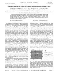
The perfectly plastic ice-sheet model can be used to demonstrate how the HMB-feedback<br />
leads to hysteresis when we consider the response <strong>of</strong> a bounded ice-sheet to <strong>climate</strong><br />
change. Suppose that the specific balance rate is a linear function <strong>of</strong> height:<br />
b n = β (h - E) , (2.11)<br />
where E is the equilibrium-line altitude and β the balance gradient (assumed to be<br />
constant). Now the total mass budget <strong>of</strong> an ice cap will be positive when<br />
h > E (2.12)<br />
So for h < E an ice sheet cannot exist. However, in the case that h > E > 0 a situation<br />
without an ice sheet also represenst an equilibrium state. For E < 0 there has to be an ice<br />
sheet.<br />
Altogether this can be visualised in a solution diagram (Fig. 2.2), showing the<br />
equilibrium states as a function <strong>of</strong> the climatic conditions. In this simple model the ice<br />
sheet can have only two states (for given L). Climate change is represented <strong>by</strong> a shift <strong>of</strong><br />
the equilibrium line. The critical points are shown <strong>by</strong> black dots.<br />
9
Fig. 2.2<br />
ice volume<br />
•<br />
0<br />
(cold)<br />
•<br />
E<br />
0 (warm)<br />
h mean<br />
Problems<br />
• The mean ice thickness for a perfectly plastic ice sheet can be written as H = c L 1/2 .<br />
Find the constant c.<br />
• Suppose that a perfectly plastic ice sheet is axi-symmetrical rather than 'onedimensional'.<br />
How would this affect the pr<strong>of</strong>ile?<br />
• An axi-symmetric perfectly plastic ice sheet has radius R. Find an expression for the<br />
vertical mean ice velocity u(r). Assume that the specific balance rate b is constant (and<br />
positive). There is a problem at r=R. Can you solve it?<br />
• For the Greenland ice sheet the mean value <strong>of</strong> E is about 1200 m, for the Antarctic ice<br />
sheet the equilibrium line is 'below sea level'. Can you locate these ice sheets on the<br />
solution diagram <strong>of</strong> Fig. 2.2?<br />
10
3. A simple <strong>glacier</strong> model<br />
We consider a <strong>glacier</strong> that has a uniform width, rests on a bed with a constant slope s,<br />
and behaves perfectly plastically in 'a global sense' (Fig. 3.1).<br />
Fig. 3.1<br />
Altitude<br />
h = b + H<br />
b = b<br />
0<br />
- sx<br />
equilibrium line<br />
L<br />
x<br />
The specific balance is written as<br />
b = β (h - E) , (3.1)<br />
where E is the equilibrium-line altitude and β the balance gradient (assumed to be<br />
constant). The <strong>glacier</strong> is in balance when the total mass budget is zero:<br />
L<br />
b n dx = β<br />
0<br />
0<br />
L<br />
(H + b 0 - s x - E) dx = 0<br />
. (3.2)<br />
Solving for <strong>glacier</strong> length L yields:<br />
L = 2 (H m + b 0 - E)<br />
s<br />
. (3.3)<br />
In this expression H m is the mean ice thickness. Note that the solution does not depend<br />
on the balance gradient! The next step is to find an equation for H m . We use again the<br />
concept <strong>of</strong> perfect plasticity:<br />
H m =<br />
τ 0<br />
ρ g s<br />
. (3.4)<br />
Substituting this in eq. (3.3) yields:<br />
11
L = 2 s<br />
τ 0<br />
ρ g s + b 0 - E . (3.5)<br />
The solution is shown in Fig. 3.2 (parameter values b 0 -E = 500 m, τ 0 /ρ g = 10 m). For<br />
reference the solution for zero ice thickness is also plotted. In this case the intercept <strong>of</strong><br />
the equilibrium line and bed is simply at x = L/2. For the full solution ice thickness<br />
increases with decreasing slope, which implies an upward shift <strong>of</strong> the equilibrium point<br />
(intercept <strong>of</strong> equilibrium line and <strong>glacier</strong> surface). There is no solution for a flat bed,<br />
unless the equilibrium line is allowed to slope upwards.<br />
Fig. 3.2<br />
80<br />
60<br />
L (km)<br />
40<br />
20<br />
full solution<br />
0<br />
H m<br />
= 0<br />
-20<br />
0 0.05 0.1 0.15 0.2 0.25<br />
Slope <strong>of</strong> bed<br />
The simple model can be used to make an order-<strong>of</strong>-magnitude estimate <strong>of</strong> <strong>climate</strong><br />
sensitivity. Differentiating Eq. (3.5) with respect to E yields:<br />
d L<br />
dE<br />
= - 2 s<br />
. (3.6)<br />
So <strong>glacier</strong>s on a bed with a smaller slope are more sensitive in an absolute sense. It is<br />
tempting to use eq. (3.6) to make a first-order estimate <strong>of</strong> the response <strong>of</strong> <strong>glacier</strong> length<br />
to a change in free atmospheric temperature Ta. We assume that the equilibrium-line is<br />
linked to this temperature, which implies that d E/d T a = -γ -1 . Here γ is the temperature<br />
lapse rate in the atmosphere, typically -0.007 K km -1 ). It follows that<br />
12
d L<br />
d T a<br />
= ∂ L<br />
∂ E<br />
d E<br />
d T a<br />
= 2<br />
γ s . (3.7)<br />
So we have arrived at the remarkable result that, for the given simple model, only two<br />
parameters are needed to estimate the sensitivity <strong>of</strong> <strong>glacier</strong> length to atmospheric<br />
temperature, namely, the characteristic bed slope and the temperature lapse rate! Fig. 3.3<br />
shows d L/d T a in dependence <strong>of</strong> s for the above mentioned value<strong>of</strong> the lapse rate. Larger<br />
valley <strong>glacier</strong>s typically have mean slopes between 0.1 and 0.2, implying that a 1 K<br />
temperature rise would lead to a 1 to 3 km decrease in <strong>glacier</strong> length. These figures<br />
appear reasonable, and we can conclude that the simple <strong>glacier</strong> model provides an<br />
interesting first-order description <strong>of</strong> the relation between <strong>climate</strong> change and <strong>glacier</strong><br />
response.<br />
Fig. 3.3<br />
0<br />
dL/dT a<br />
(km K -1 )<br />
-2<br />
-4<br />
-6<br />
-8<br />
large valley <strong>glacier</strong>s<br />
0.05 0.1 0.15 0.2 0.25<br />
Slope <strong>of</strong> bed<br />
Problems:<br />
• The absolute change in <strong>glacier</strong> length for a given change in E is larger when the slope<br />
is smaller. However, does this also apply to the relative change in L?<br />
• What are, in your judgement, the largest deficiencies <strong>of</strong> the model presented above?<br />
13
4. A <strong>glacier</strong> model with a more complicated geometry<br />
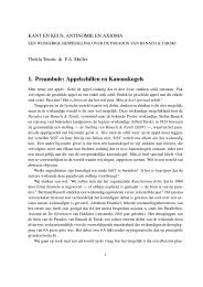
Glaciers having a constant width are very rare. Larger valley <strong>glacier</strong>s <strong>of</strong>ten show a pattern<br />
<strong>of</strong> a relatively wide accumulation basin and a narrower snout that flows into the valley.<br />
Examples are shown in Fig. 4.1.<br />
Fig. 4.1<br />
Nigardsbreen<br />
Abramov Glacier<br />
N<br />
N<br />
1800<br />
400<br />
600<br />
800<br />
1000<br />
1200<br />
1600<br />
1400<br />
1400<br />
2200<br />
1800<br />
1000<br />
800<br />
1800<br />
2000<br />
1952 m<br />
600<br />
2200<br />
2600<br />
400<br />
2400<br />
2987 m<br />
2 km<br />
2901 m<br />
2 km<br />
To handle such a situation we use a very schematic geometry in which the <strong>glacier</strong> consists<br />
<strong>of</strong> two parts having a different width. Again, L is the <strong>glacier</strong> length and the upper basin<br />
has length L ub (Fig. 4.2).<br />
Fig. 4.2<br />
L ub<br />
L<br />
0<br />
x<br />
14
For L < L ub the solution is given <strong>by</strong> eq. (3.3):<br />
L = 2 (H + b 0 - E)<br />
s<br />
. (4.1)<br />
When the mass budget <strong>of</strong> the upper basin is positive L will be larger than Lub. The length<br />
<strong>of</strong> the <strong>glacier</strong> is then determined <strong>by</strong><br />
L ub L<br />
(H + b 0 - s x - E) dx + ξ (H + b 0 - s x - E) dx = 0<br />
0<br />
L ub<br />
. (4.2)<br />
Here ξ is the width <strong>of</strong> the <strong>glacier</strong> tongue divided <strong>by</strong> the width <strong>of</strong> the upper basin.<br />
Evaluating the integrals yields:<br />
- 1 2 ξ s L2 + ξ (H + b 0 - E) L + (1 - ξ) (H + b 0 - E) L ub - 1 2 s (1 - ξ) L ub<br />
2 = 0 (4.3)<br />
This is a quadratic equation for L which is easily solved:<br />
L = - 1 s<br />
E' + E' 2 + 2 s 1-ξ<br />
ξ<br />
1/2<br />
E' L ub + 1 2 s L ub<br />
2<br />
(4.4)<br />
In this expression E' = E - b 0 - H (note that E' < 0).<br />
The solution is illustrated in Fig. 4.3. In this example the upper basin has a length <strong>of</strong><br />
5 km. Other parameter values are b 0 =2000 m, s=0.1, H=100 m. L is plotted as a<br />
function <strong>of</strong> E for three different values <strong>of</strong> ξ. For ξ=0.25, the width <strong>of</strong> the upper basin is<br />
four times that <strong>of</strong> the <strong>glacier</strong> tongue.<br />
Fig. 4.3<br />
20<br />
L (km)<br />
15<br />
10<br />
ξ =4<br />
ξ=1<br />
ξ =0.25<br />
largest sensitivity<br />
5<br />
0<br />
1400 1500 1600 1700 1800 1900 2000<br />
E (m)<br />
15
In this case the <strong>glacier</strong> length increases rapidly when the equilibrium line sinks below<br />
1850 m. A clear maximum <strong>of</strong> dL/dE exists when the <strong>glacier</strong> starts to form the snout.<br />
When the equilibrium line sinks still further, in the end dL/dE will approach the value <strong>of</strong><br />
the original model <strong>glacier</strong> <strong>of</strong> uniform width. When the lower part <strong>of</strong> the <strong>glacier</strong> is wider<br />
than the upper part the opposite is seen. The sensitivity is at a minimum when the budget<br />
<strong>of</strong> the upper basin is just positive.<br />
In conclusion we can state that <strong>glacier</strong>s with a narrow tongue are the ones that are most<br />
sensitive to <strong>climate</strong> change, especially when the <strong>glacier</strong> front is just below the upper<br />
basin.<br />
16
5. A volume time scale for valley <strong>glacier</strong>s<br />
A time scale for the adjustment <strong>of</strong> <strong>glacier</strong>s to <strong>climate</strong> change can be derived from the<br />
requirement <strong>of</strong> mass continuity (Jóhanesson et al, 1989; Haeberli and Hoelzle, 1995).<br />
We perform a linear perturbation analysis. Conservation <strong>of</strong> ice volume V can be<br />
expressed as<br />
d V<br />
d t<br />
= d A H m<br />
d t<br />
= H m d A<br />
d t<br />
+ A dH m<br />
d t<br />
. (5.1)<br />
Here A is the <strong>glacier</strong> area and H m the mean ice thickness. Now we write<br />
V = V 0 + V', A = A 0 +A' and H m = H m,0 + H m ', where the reference state is defined<br />
as (V 0 , A 0 , H m,0 ). By substitution in eq. (5.1) and <strong>by</strong> neglecting higher-order terms we<br />
then obtain the perturbation equation<br />
d V'<br />
d t<br />
= H m,0 d A'<br />
d t<br />
+ A 0 dH m '<br />
d t<br />
. (5.2)<br />
Next we assume (see Fig. 7.1):<br />
A' = w f L' , (5.3)<br />
Here w f is the characteristic width <strong>of</strong> the <strong>glacier</strong> tongue.<br />
Fig. 6.1.<br />
L'<br />
total <strong>glacier</strong><br />
area A<br />
w f<br />
flowline<br />
If the mean thickness <strong>of</strong> the <strong>glacier</strong> does not change we have for the change <strong>of</strong> ice volume<br />
with time<br />
17
d V'<br />
d t<br />
= w f H m,0 d L'<br />
d t<br />
= amount <strong>of</strong> mass added . (5.4)<br />
In a perturbation analysis we have two contributions to the mass added to or removed<br />
from the <strong>glacier</strong>:<br />
change <strong>of</strong> volume = A 0 B' + w f B f L' . (5.5)<br />
B' is the perturbation <strong>of</strong> the balance rate (constant over the <strong>glacier</strong>), and B f the<br />
characteristic balance rate at the <strong>glacier</strong> front. The first term is simply the amount <strong>of</strong> ice<br />
added or removed <strong>by</strong> the balance perturbation on the reference <strong>glacier</strong> area. The second<br />
term is the amount <strong>of</strong> ice lost or gained because the length <strong>of</strong> the <strong>glacier</strong> deviates from that<br />
<strong>of</strong> the reference state. Combining eqs. (5.4)-(5.6) yields<br />
d L'<br />
d t<br />
=<br />
A 0<br />
w f H m,0<br />
B' +<br />
B f<br />
H m,0<br />
L' . (5.7)<br />
The equilibrium state is obtained <strong>by</strong> setting the time derivative to zero. This gives:<br />
L' = - A 0<br />
w f B f<br />
B' . (5.8)<br />
The response time for <strong>glacier</strong> length according to this model is apparently<br />
t L = -<br />
H m,0<br />
B f<br />
. (5.9)<br />
Some examples on response times are given in the table below. The quantities marked<br />
with • are the input data. Eq. (6.1) has been used to calculate H o . The response time is<br />
then obtained from eq. (5.9).<br />
•Ao<br />
•Lo<br />
•s<br />
•β<br />
Ho<br />
•W f<br />
•B f<br />
t L<br />
(km 2 )<br />
(km)<br />
(m 2 yr -1 )<br />
(m)<br />
(m)<br />
(m yr -1 )<br />
(yr)<br />
Nigardsbreen 48.8 10.4 0.13 0.0078 125 500 -10 13<br />
Abramov Glac. 25.9 9.1 0.09 0.0055 136 700 -4 34<br />
Rhonegletscher 18.5 9.8 0.13 0.0066 122 900 -5 24<br />
Franz-Josef Gl. 36 11.4 0.21 0.0125 107 600 -22 5<br />
Aletschgletscher 86.8 24.7 0.1 0.0066 215 1200 -8 27<br />
Ob. Grindelw.gl. 10.1 5.0 0.25 0.0066 65 500 -7 9<br />
18
Problem:<br />
• The time scale derived above is not very accurate, because it ignores the HMBfeedback.<br />
Repeat the analysis and include the HMB-feedback <strong>by</strong> assuming that<br />
H m ' = η L'. Find η <strong>by</strong> linearising eq. (6.1). Calculate the newly derived time scale<br />
for the <strong>glacier</strong>s in the table. Conclusion?<br />
19
6. Including feedback between <strong>glacier</strong> length and ice thickness<br />
In the analysis <strong>of</strong> section 3 we made thickness a function <strong>of</strong> the bed slope, but not <strong>of</strong> the<br />
<strong>glacier</strong> length. This is an obvious shortcoming. A more advanced analysis can be made<br />
<strong>by</strong> using the relation:<br />
H m =<br />
1/2<br />
µ L<br />
, (6.1)<br />
1+ ν s<br />
where µ and ν are positive constants. Actually, eq. (6.1) fits rather well results form a<br />
numerical <strong>glacier</strong> model in which s and L are systematically varied (Oerlemans, 2001).<br />
Note that for s = 0 eq. (6.1) reduces to the relation between ice thickness and <strong>glacier</strong>s<br />
length for a perfectly plastic ice sheet on a flat bed (section 2). In the simple model, the<br />
expression for L was:<br />
L = 2 (H m + b 0 - E)<br />
s<br />
. (6.2)<br />
By substituting eq. (6.1) we obtain (E ' = E -b 0 ):<br />
L = 2 s<br />
1/2<br />
µ L<br />
- E ' . (6.3)<br />
1 + ν s<br />
This quadratic equation is most conveniently solved <strong>by</strong> setting N = L 1/2 . We then have<br />
N 2 -<br />
2 µ 1/2<br />
s (1 + ν s) 1/2<br />
N + 2 E '<br />
s<br />
= 0 . (6.4)<br />
The determinant is<br />
Det =<br />
4 µ<br />
s 2 (1 + ν s)<br />
- 8 E '<br />
s<br />
. (6.5)<br />
Real solutions exist only when Det ≥ 0. The first term is always positive. Therefore a real<br />
solution exists even for small positive values <strong>of</strong> E ', that is, when the equilibrium line is<br />
higher than the highest part <strong>of</strong> the bed at x = 0, but below the <strong>glacier</strong> surface. This<br />
nonlinearity, <strong>of</strong> course, reflects the HMB-feedback. The solution for L reads<br />
L =<br />
µ 1/2<br />
s (1 + ν s) 1/2 ± µ<br />
s 2 (1 + ν s)<br />
- 2 E '<br />
s<br />
1/2<br />
2<br />
. (6.6)<br />
20
Note that values <strong>of</strong> L for which N < 0 are spurious and should not be considered.<br />
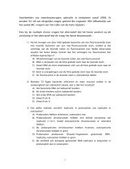
An example is shown in Fig. 6.1. Parameter values are: µ = 9 m, ν = 20, s = 0.06 .<br />
Because L = 0 is a stable solution for E ' > 0 (equilibrium line above the bed<br />
everywhere), there are two stable branches and one unstable branch (dotted). In terms <strong>of</strong><br />
catastrophe theory this model represents a fold, but because we add the condition that L<br />
should be positive it appears as a distorted cusp. The branching <strong>of</strong> the steady-state<br />
solutions that shows up here was in fact found numerically a long time ago (Oerlemans,<br />
1981). It should also be mentioned that the dynamics <strong>of</strong> the present <strong>glacier</strong> model are<br />
similar to those <strong>of</strong> a perfectly plastic ice sheet on a flat bed with a sloping equilibrium line<br />
Weertman (1961).<br />
The range <strong>of</strong> E '-values for which two stable solutions exist is<br />
0 ≤ E ' < E ' crit , (6.7)<br />
where the critical point E' crit is found <strong>by</strong> setting Det = 0:<br />
E ' crit =<br />
µ<br />
2 s (1 + ν s)<br />
. (6.8)<br />
Therefore, for increasing slope <strong>of</strong> the bed, the HMB-feedback becomes weaker and the<br />
critical point approaches the origin. The result for the linear <strong>analytical</strong> model is also<br />
shown. In this caseτ 0 /ρg was set to 9 m, because this is consistent with eq. (6.1) for<br />
s = 0. The squares in Fig. 6.1 shows the dependence <strong>of</strong> <strong>glacier</strong> length on E' as found <strong>by</strong><br />
a numerical plane-shear model for a <strong>glacier</strong> <strong>of</strong> constant width. Clearly, the nonlinear<br />
<strong>analytical</strong> model matches the numerical result very well.<br />
Fig. 6.1.<br />
14<br />
12<br />
10<br />
L (km)<br />
8<br />
6<br />
4<br />
linear model<br />
2<br />
0<br />
nonlinear model<br />
•<br />
•<br />
-200 -150 -100 -50 0 50<br />
E' (m)<br />
21
From the foregoing analysis it is clear that the bed slope is a very important parameter.<br />
For smaller slopes (ice sheets / ice caps) nonlinear effects are more important than for<br />
larger slopes (valley <strong>glacier</strong>s). To classify <strong>glacier</strong> beds with a characteristic slope only<br />
provides not mroe than a schematic picture, <strong>of</strong> course. Nevertheless, it is instructive to<br />
compae curves for different slopes and to speculate how existing <strong>glacier</strong>s and ice caps<br />
might fit in (see Fig. 6.2).<br />
Fig. 6.2<br />
1 10 6<br />
s=0.006<br />
8 10 5<br />
L (m)<br />
6 10 5<br />
4 10 5<br />
• Greenland<br />
2 10 5<br />
0<br />
s=0.02<br />
s=0.1 Aletschgl.<br />
Vatnajökull<br />
•<br />
-1000 -750 -500 -250 0 250 500 750<br />
E' (m)<br />
22
7. Steady state ice-sheet pr<strong>of</strong>iles<br />
The perfectly plastic ice-sheet model can be improved <strong>by</strong> calculating the pr<strong>of</strong>ile for simple<br />
plane shear (Vialov, 1958). In this case the deviatoric stress tensor S ij has only one<br />
nonzero component:<br />
S xz (z) = (H-z) ρ g sin α . (7.1)<br />
Here H is the ice thickness, z the height above the bed, ρ ice density and α the surface<br />
n<br />
slope. This can be combined with Glen's law for simple shear (du/dz = 2 A S xz ) to give<br />
du<br />
dz<br />
= 2 A (H-z) ρ g sin α n . (7.2)<br />
Integrating this equation twice with respect to z yields the vertical mean 'horizontal' ice<br />
velocity U<br />
U = A* H n+1 sin α n + U s (7.3)<br />
In this equation U s is the sliding velocity. A* is the effective flow parameter, which can<br />
be expressed in A, ρ, g and n (see Problems).<br />
Next we consider an axi-symmetric configuration (Fig. 7.1). The vertically-integrated<br />
continuity equation then takes the form:<br />
∂ H<br />
∂ t<br />
= -∇⋅(H U) + b → ∂ H<br />
∂ t<br />
= - ∂(r H U r )<br />
r ∂ r<br />
+ b (7.4)<br />
therefore for the steady state we find:<br />
d (r H U r ) = b r d r → U r = b 2 H-1 r (7.5)<br />
Fig. 7.1<br />
H<br />
φ<br />
R<br />
r<br />
23
We assume that the ice-sheet base is flat and replace sin α <strong>by</strong> dH/dx. With zero sliding<br />
velocity we then have:<br />
U r = - A* H n+1 d H<br />
d r<br />
n<br />
. (7.6)<br />
Now the velocity can be eliminated <strong>by</strong> combining eqs. (7.5) and (7.6):<br />
1+2/n<br />
H<br />
dH<br />
dr<br />
1/n<br />
= - b r<br />
1/n . (7.7)<br />
2 A*<br />
Integration with respect to r yields<br />
n<br />
2n+2 H 2+2/n - H 0<br />
2+2/n = - n<br />
n+1<br />
1/n<br />
b<br />
2 A*<br />
r 1+1/n , (7.8)<br />
or<br />
H 2+2/n - H 0<br />
2+2/n = - 2<br />
1/n<br />
b<br />
2 A*<br />
r 1+1/n . (7.9)<br />
Next we have to apply a boundary condition, namely H = 0 at r = R. This leads to a<br />
relation between the ice thickness in the centre and the ice-sheet radius:<br />
H 0<br />
2+2/n = 2<br />
1/n<br />
b<br />
2 A*<br />
R 1+1/n . (7.10)<br />
The final solution then becomes<br />
H(r) = 2 n/(2n+2) b/(2A*) 1/(2n+2) R 1+1/n - r 1+1/n n/(2n+2) . (7.11)<br />
The most commonly used exponent in Glen's law is 3. In this case we have<br />
H(r) = 2 3/8 b/(2A*) 1/8 R 4/3 - r 4/3 3/8 . (7.12)<br />
The solution is shown in Fig. 7.2, together with the pr<strong>of</strong>ile <strong>of</strong> a pefectly plastic ice sheet<br />
as derived in section 2. The plane shear solution is shown for two values <strong>of</strong> A*: one for<br />
which the height at the centre is equal to that <strong>of</strong> the pefectly plastic solution, and one in<br />
which the mean ice thickness is approximately equal to the mean ice thockness for the<br />
perfectly plastic ice sheet.<br />
24
Fig. 7.2<br />
3500<br />
3000<br />
2500<br />
h (m)<br />
2000<br />
1500<br />
1000<br />
500<br />
perfectly plastic<br />
plane shear 1<br />
plane shear 2<br />
0<br />
0 200 400 600 800 1000 1200 1400 1600<br />
r (km)<br />
A few interesting conclusions can be draw from the plane-shear solution. For n=3 eq.<br />
(7.10) reads<br />
H 0 = 2<br />
1/8<br />
b<br />
2 A*<br />
R 1/2 (7.13)<br />
This shows that the dependence <strong>of</strong> the ice thickness on the accumulation rate is quite<br />
weak. Halving the accumulation rate reduces the ice thickness <strong>by</strong> only 8%. The same<br />
applies to the relation between ice thickness and flow parameter. On the other hand, the<br />
dependence on ice-sheet radius is larger. Halving the radius reduces the ice thickness <strong>by</strong><br />
30%.<br />
It is hard to judge which model performs best. It is clear that the perfectly plastic model<br />
is not very accurate in the central part <strong>of</strong> an ice sheet. However, in many applications this<br />
does not matter at all. One can try to check the validity <strong>of</strong> the pr<strong>of</strong>iles <strong>by</strong> comparison with<br />
observations. This does not give definite answers as to which pr<strong>of</strong>ile performs best (Van<br />
der Veen, 1999). The less steep slope <strong>of</strong> the parabolic pr<strong>of</strong>ile closer to the ice edge seems<br />
more realistic in many cases, albeit for the wrong reason (in reality s<strong>of</strong>ter ice and sliding<br />
over deformable beds leads to reduced ice thickness).<br />
It is noteworthy that the dependence <strong>of</strong> ice thickness on the radius is the same for the<br />
plane-shear and perfectly-plastic <strong>models</strong>. Altogether, when interest is in the large-scale<br />
response <strong>of</strong> ice sheets to environmental change, and when changes in ice volume are<br />
expected to be mainly the result <strong>of</strong> changes in R, then the perfectly plastic model is not a<br />
bad choice.<br />
25
Problems:<br />
• Find an expression for A* in eq. (7.3).<br />
• Suppose that the accumulation rate is not constant but increases with r: b = B R r/R.<br />
Find a new expression for the plane-shear solution and compare with the case <strong>of</strong><br />
constant b.<br />
• The flow parameter A depends on ice temperature, approximately following the<br />
relation A = A 0 exp(-Q/RT). Find out for the plane-shear solution <strong>by</strong> how much the<br />
maximum ice thickness changes when the characteristic ice temperature drops from<br />
275 K to 285 K. Parameter values: A 0 = 1.14⋅10 10 Pa -3 yr -1 , Q = 100 kJ mol -1 .<br />
• We design a schematic mass continuity model for a marine ice sheet. Suppose that the<br />
ice sheet rests on a bed that slopes downwards at a constant rate: b = b 0 - s r and that<br />
the accumulation rate is constant (a). The ice-sheet edge is in the sea, and the<br />
azimuthally averaged ice velocity is proportional to the water depth d (so U R = f * d).<br />
Find an expression for the total mass budget <strong>of</strong> the ice sheet and solve for the icesheet<br />
radius R.<br />
Apply the model to the West Antarctic ice sheet (set b 0 = 0 for simplicity) and try to<br />
fimd out the sensitivity <strong>of</strong> R to changes in accumulation rate (use<br />
R = 600 km, f = 1 yr -1 , a = 0.25 m yr -1 ).<br />
REFS<br />
Haeberli W. and M. Hoelzle (1995): Application <strong>of</strong> inventory data for estimating<br />
characteristics <strong>of</strong> and regional <strong>climate</strong>-change effects on mountain <strong>glacier</strong>s: a pilot<br />
study with the European Alps. Annals <strong>of</strong> Glaciology 21, 206-212.<br />
Jóhannesson T., C.F. Raymond and E.D. Waddington (1989): Time-scale for<br />
adjustment <strong>of</strong> <strong>glacier</strong>s to changes in mass balance. Journal <strong>of</strong> Glaciology 35, 355-<br />
369.<br />
Oerlemans J. (1981): Some basic experiments with a vertically-integrated ice-sheet<br />
model. Tellus 33, 1-11.<br />
Vialov S.S. (1958): Regularities <strong>of</strong> glacial shields movement and the theory <strong>of</strong> plastic<br />
viscous flow. International Association <strong>of</strong> Hydrology, Scientific Publication 47, 266-<br />
275.<br />
Weertman J. (1961): Stability <strong>of</strong> ice-age ice sheets. Journal <strong>of</strong> Geophysical Research<br />
66, 3783-3792.<br />
26
Problem HMB-feedback and response time (P 1)<br />
Conservation <strong>of</strong> ice volume V can be expressed as<br />
d V<br />
d t<br />
= d A H m<br />
d t<br />
= H m d A<br />
d t<br />
+ A dH m<br />
d t<br />
. (P 1.1)<br />
Here A is the <strong>glacier</strong> area and H m the mean ice thickness. Now we write<br />
V = V 0 + V', A = A 0 +A' and H m = H m,0 + H m ', where the reference state is defined<br />
as (V 0 , A 0 , H m,0 ). By neglecting higher-order terms we then obtain the perturbation<br />
equation<br />
d V'<br />
d t<br />
= H m,0 d A'<br />
d t<br />
+ A 0 dH m '<br />
d t<br />
. (P 1.2)<br />
Again we assume:<br />
A' = w f L' , (P 1.3)<br />
Here w f is the characteristic width <strong>of</strong> the <strong>glacier</strong> tongue. Now we include the height-mass<br />
balance feedback <strong>by</strong> assuming that the change in mean thickness is proportional to the<br />
change in <strong>glacier</strong> length:<br />
H m ' = η L' . (P 1.4)<br />
So for the change <strong>of</strong> ice volume with time we find<br />
d V'<br />
d t<br />
= η A 0 + w f H m,0 d L'<br />
d t<br />
= amount <strong>of</strong> mass added . (P 1.5)<br />
We now have three contributions to the mass added to or removed from the <strong>glacier</strong>:<br />
change <strong>of</strong> volume = A 0 B' + A 0 β H m ' + w f B f L' = A 0 B' + A 0 β η' + w f B f L' .<br />
(P 1.6)<br />
B' is the perturbation <strong>of</strong> the balance rate (constant over the <strong>glacier</strong>), β the balance gradient<br />
and B f the characteristic balance rate at the <strong>glacier</strong> front. The first term is simply the<br />
amount <strong>of</strong> ice added or removed <strong>by</strong> the balance perturbation on the reference <strong>glacier</strong> area.<br />
The second term represents the feedback between balance rate and surface elevation. The<br />
third term is the amount <strong>of</strong> ice lost or gained because the length <strong>of</strong> the <strong>glacier</strong> deviates<br />
from that <strong>of</strong> the reference state. Combining the equations yields<br />
27
d L'<br />
d t<br />
=<br />
A 0<br />
η A 0 + w f H m,0<br />
B' + η β A 0 + w f B f<br />
η A 0 + w f H m,0<br />
L' . (P 1.7)<br />
The equilibrium state is obtained <strong>by</strong> setting the time derivative to zero. This gives:<br />
A<br />
L' = - 0 B'<br />
. (P 1.8)<br />
η β A 0 + w f B f<br />
The response time for <strong>glacier</strong> length according to this model is apparently<br />
t L = - η A 0 + w f H m,0<br />
η β A 0 + w f B f<br />
. (P 1.9)<br />
Some examples on response times are given in the table below. The quantities marked<br />
with • are the input data. Eq. (6.1) has been used to calculate H o and η. The response<br />
time is then obtained from eq. (P 1.9). The last column shows the response time in the<br />
absence <strong>of</strong> the HMB-feedback. Apparently for most <strong>glacier</strong>s the HMB-feedback is<br />
important.<br />
•Ao<br />
•Lo<br />
•s<br />
•β<br />
Ho<br />
η<br />
•W f<br />
•B f<br />
t L<br />
t L (η=0)<br />
(km 2 )<br />
(km)<br />
(m 2 yr -1 )<br />
(m)<br />
(m)<br />
(m yr -1 )<br />
(yr)<br />
(yr)<br />
Nigardsbreen 48.8 10.4 0.13 0.0078 125 0.0060 500 -10 129 13<br />
Abramov Glac. 25.9 9.1 0.09 0.0055 136 0.0075 700 -4 167 34<br />
Rhonegletscher 18.5 9.8 0.13 0.0066 122 0.0062 900 -5 60 24<br />
Franz-Josef Gl. 36 11.4 0.21 0.0125 107 0.0047 600 -22 21 5<br />
Aletschgletscher 86.8 24.7 0.1 0.0066 215 0.0044 1200 -8 90 27<br />
Ob. Grindelw.gl. 10.1 5.0 0.25 0.0066 65 0.0065 500 -7 32 9<br />
28
Problem ice-sheet pr<strong>of</strong>ile (P 2)<br />
For the steady-state radial velocity we now have:<br />
d (r H U r ) = b R r2<br />
R<br />
d r → U r =<br />
b R<br />
3 R H-1 r 2 (P 2.1)<br />
This can be combined again with the expression for the vertical mean ice velcocity in the<br />
case <strong>of</strong> simple shearing flow:<br />
U r = - A* H n+1 d H<br />
d r<br />
n<br />
(P 2.2)<br />
We get<br />
1+2/n<br />
H<br />
dH<br />
dr<br />
= -<br />
1/n<br />
b R<br />
3 R A*<br />
r 2/n (P 2.3)<br />
Integration with respect to r yields<br />
n<br />
2n+2 H 2+2/n - H 0<br />
2+2/n = - n<br />
n+2<br />
1/n<br />
b R<br />
3 R A*<br />
r 1+2/n , (P 2.4)<br />
or<br />
H 2+2/n - H 0<br />
2+2/n = - 2n+2<br />
n+2<br />
1/n<br />
b R<br />
3 R A*<br />
r 1+2/n . (P 2.5)<br />
Next we have to apply a boundary condition, namely H = 0 at r = R. This leads to a<br />
relation between the ice thickness in the centre and the ice-sheet radius:<br />
H 0<br />
2+2/n = 2n+2<br />
n+2<br />
1/n<br />
b R<br />
3 R A*<br />
R 1+2/n . (P 2.6)<br />
The final solution then becomes<br />
H(r) = 2n+2<br />
n+2<br />
n/(2n+2)<br />
b R /(3 R A*) 1/(2n+2) R 1+2/n - r 1+2/n n/(2n+2) . (P 2.7)<br />
For n=3 we have:<br />
29
H(r) = 8/5 3/8 b R /(3 R A*) 1/8 R 5/3 - r 5/3 3/8 (P 2.8)<br />
3500<br />
3000<br />
2500<br />
b=const<br />
b=b R<br />
r/R<br />
2000<br />
H (m)<br />
1500<br />
1000<br />
500<br />
0<br />
-500<br />
0 500 1000 1500 2000<br />
r (km)<br />
30
Problem West Antarcic ice sheet (P 3)<br />
The mass budget equation is obtained <strong>by</strong> setting the total accumulation equal to the total<br />
flux across the grounding line. This flux equals the ice velocity times the outlet cross<br />
section. Therefore<br />
π a R = 2 π R f * ρ w<br />
ρ i<br />
d 2 = 2 π R f d 2 (P 3.1)<br />
The water depth at the grounding line equals b 0 - s R, so we have<br />
d 2 = b 0<br />
2 + s<br />
2 R<br />
2 - 2 b0 s R (P 3.2)<br />
Combining yields<br />
2 f s 2 R 2 - (4 b 0 f s + a) R + 2 f b 0<br />
2 = 0 (P 3.3)<br />
Special case: b 0 = 0 (a purely marine ice sheet). So the highest point <strong>of</strong> the continent is<br />
just at sea level. Eq. (P 2.3) reduces to<br />
2 f s 2 R 2 - a R = 0 (P 3.4)<br />
→ R = a<br />
2 f s 2 (P 3.5)<br />
Application to the WAIS (R = 600 km, f = 1 yr -1 , a = 0.25 m yr -1 ):<br />
1/2<br />
→ s = a = 0.25<br />
1/2 = 0.00046 (P 3.6)<br />
2 f R 2 x 1 x 600,000<br />
Sensitivity to changes in accumulation rate:<br />
∂R<br />
∂a = 1<br />
2 f s 2 = 2.37x106 = 23.7 km/% (P 3.7)<br />
31