TURBIDITY SENSOR FOR UNDERWATER APPLICATIONS Sensor ...

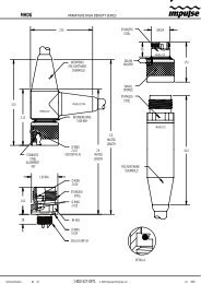
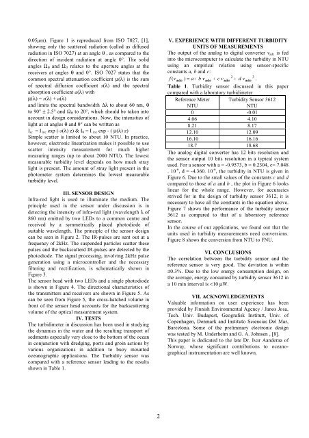
0.05µm). Figure 1 is reproduced from ISO 7027, [1],
showing only the scattered radiation (called as diffused
radiation in ISO 7027) at an angle θ , as compared to the
direction of incident radiation at angle 0°. The solid
angles Ω θ and Ω 0 relates to the aperture angles at the
receivers at angles θ and 0°. ISO 7027 states that the
common spectral attenuation coefficient µ(λ) is the sum
of spectral diffusion coefficient s(λ) and the spectral
absorption coefficient a(λ) with
µ(λ) = s(λ) + a(λ)
and limits the spectral bandwidth ∆λ to about 60 nm, θ
to 90° ± 2.5° and Ω θ to 20°, which should be taken into
account in design considerations. Now, the intensities of
light at at angles θ and 0° can be written as
I sc = I inc exp (-s(λ) z) & I 0 = I inc exp - ( µ(λ) z)
Simple scatter is limited to about 10 NTU. In practice,
however, electronic linearization makes it possible to use
scatter intensity measurement for much higher
measuring ranges (up to about 2000 NTU). The lowest
measurable turbidity level depends on how much stray
light is present. The amount of stray light present in the
photometer system determines the lowest measurable
turbidity level.
III. SENSOR DESIGN
Infra-red light is used to illuminate the medium. The
principle used in the sensor under discussion is in
detecting the intensity of infra-red light (wavelength λ of
860 nm) emitted by two LEDs to a common centre and
received by a symmetrically placed photodiode of
suitable wavelength. The principle of the sensor design
can be seen in Figure 2. The IR-pulses are sent out at a
frequency of 2kHz. The suspended particles scatter these
pulses and the backscatterd IR-pulses are detected by the
photodiode. The signal processing, involving 2kHz pulse
generation using a microcontroller and the necessary
filtering and rectification, is schematically shown in
Figure 3.
The sensor head with two LEDs and a single photodiode
is shown in Figure 4. The directional characteristics of
the transmitters and receivers are shown in Figure 5. As
can be seen from Figure 5, the cross-hatched volume in
front of the sensor head accounts for the backscattering
volume of the optical measurement system.
IV. TESTS
The turbidimeter in discussion has been used in studying
the dynamics in the water and the resulting transport of
sediments especially very close to the bottom of the ocean
in conjunction with dredging, ports and groin actions by
various organizations in addition to buoy mounted
oceanographic applications. The Turbidity sensor was
compared with a reference sensor leading to the results
shown in Table 1.
V. EXPERIENCE WITH DIFFERENT TURBIDITY
UNITS OF MEASUREMENTS
The output of the analog to digital converter v adc is fed
into the microcomputer to calculate the turbidity in NTU
using an empirical relation using sensor-specific
constants a, b and c:
f ( v ) = a + b v + c v + d v
2
adc adc adc adc
3 .
Table 1. Turbidity sensor discussed in this paper
compared with a laboratory turbidimeter
Reference Meter Turbidity Sensor 3612
NTU
NTU
0 -0.01
4.06 4.10
8.21 8.17
12.10 12.09
16.10 16.16
18.7 18.68
The analog digital converter has 12 bits resolution and
the sensor output 10 bits resolution in a typical system
used. For a sensor with a = -0.9573, b = 0.2304, c= 7.048
. 10 -6 , d = -4.360. 10 -6 , the turbidity in NTU is given in
Figure 6. Due to the small values of the constants c and d
compared to those of a and b , the plot in Figure 6 looks
linear for the whole range. However, for accuracies
strived for in the design of turbidity sensor 3612, it is
necessary to have all the constants in the equation above.
Figure 7 shows the performance of the turbidity sensor
3612 as compared to that of a laboratory reference
sensor.
In the course of our applications, we found out that the
units used in turbidity measurements need conversions.
Figure 8 shows the conversion from NTU to FNU.
VI. CONCLUSIONS
The correlation between the turbidity sensor and the
reference sensor is very good. The deviation is within
±0.3%. Due to the low energy consumption design, on
the average, energy consumed by turbidity sensor 3612 in
a 10 min interval is