advantages and limitations of the interline power flow ... - PSCC

2 is in charge of fulfilling this demand through the
Pse1 + Pse2
= 0 constraint. Unlike VSC-1 (in the primary
system) the operation of VSC-2 (secondary system) has
its freedom degrees reduced; thus, its series voltage V C2
can compensate only partially to its own line. This is
because converter VSC-2 also has the task of regulating
the dc-link voltage. So, the P se2 component of VSC-2 is
predefined. This imposes a restriction to this line in that
mainly the quadrature component of V C2 can be specified
to control its power flow. Under this condition, the
primary system will have priority over the secondary
system in achieving its set-point requirements.
The equivalent sending and receiving-end sources in
both AC systems are regarded as stiff. The condition for
which the switch CB is closed (i.e. V 11 =V 21 ) also applies
to the analysis presented in this section.
System 1
V 11
V 12 V V P
C1
13
V
I 1 14
14
Z 11
(P
CB
se1
+P se2
) = 0
System 2
V P
C2
I 2
24
Z 21
Z 24
V 21
V 22
V 23 V 24
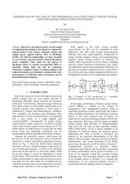
Figure 2: IPFC scheme used in the analysis
It will also be assumed that both AC systems have
identical line parameters. Likewise, it is assumed that
each converter injects an ideal sinusoidal waveform
with only its fundamental frequency [8], [9], [13]. The
steady-state power balance of the n number of converters
(same number of compensated lines) can be represented
by (1):
n
∑
i=
1
P 0
(1)
se _ i
=
As in our case n=2, we will have,
P + = 0
se1
Pse2 (2)
So for each line it can be written,
P
se1
= VC1d
I14d
+ VC1qI14q
(3)
P = V I + V I
(4)
se2
C2d
24d
C2q
From Figure 2, the following system equations can
be written:
V12d
= V14d
−VC1
d
− X14I14d
(5a)
V12 q
= V14q
−VC1
q
+ X14I14q
(5b)
V22d
= V24d
−VC
2d
− X
24I
24d
(6a)
V22 q
= V24q
−VC
2q
+ X
24I
24q
(6b)
I14 d
= k1( V11q
−V14q
+ VC1
q
)
(7a)
I14q
= k1( −V11
d
+ V14d
−VC1
d
)
(7b)
I
24 d
= k2
( V21q
−V24q
+ VC
2q
)
(8a)
= k −V
+ V V
(8b)
24q
( )
I
24q
2 21d
24d
−
C 2d
Z 14
where k
= 1
( X + )
,
1
11
X
14
k
= 1
( X
2
21
+ X
24
Equations (2) through (8) allow the main parameters
of the elementary IPFC to be calculated (Figure 2).
Unlike the GIPFC case addressed in [13], the unknown
variable V C2d will be a function of V C1 (specified). Once
computed the unknown variables (i.e. the d-q components
of V 12 , V 22 , I 14 , I 24 and V C2d ), the power flow in the
receiving-end of Systems 1 and 2, with or without the
effect of the series voltage, can be calculated through
(9).
*
S
1
= ( P1
+ jQ1
) = V14
I
(9a)
14
*
S
2
= ( P2
+ jQ
2
) = V24
I
(9b)
24
Note that System 1 will have two independently controlled
variables (i.e. V C1 , θ C1 ). Conversely, System 2
will only have one variable (V C2q ) to be independently
controlled.
3 RESULTS
The results shown in Figures 3 and 4 were obtained
using the mathematical model developed in Section 2,
in which θ C1 was varied from 0° through 360°. The area
inside the circle corresponds to the ideal region controlled
by VSC-1, which will be limited by the magnitude
of V C1 (V max C1 ). The series reactive compensation in
System 2 was set to be null (i.e. V C2q =0), thus, only the
V C2d component serves as a parameter through which
active power is passed from Converter 2 to 1. The way
how VSC-2 compensates to its own line, through its
available reactive compensation, will be shown in Section
3(c).
Q (pu)
0.2
0
-0.2
-0.4
-0.6
P 1
, Q 1
(System 1)
330°
75°
240° 60°
255°
θ C2= 0°
30°
300°
120°
150°
210°
P 2
, Q 2
(System 2)
θ C1 =0°
-0.8
0.4 0.6 0.8 1 1.2 1.4 1.6
P (pu)
Figure 3: P-Q plane (receiving-end) showing the operative
region of Systems 1 & 2 when V C1 =0.2 pu & V C2d =ƒ(V C1 )
For this particular case, both AC systems were assumed
to have similar transmission angles, i.e. δ 11_14 =
δ 21_24 = -30°. Should these angles be different, maintaining
the same V C1 = 0.2 pu, the results obtained will be
different. Such a case will also be analysed shortly after.
Notice how the power flow in System 2 is forced to
vary (P 2 ≅0.8pu → 1.2pu, Q 2 ≅-0.6pu → +0.1pu) on
account of helping to control P 1 & Q 1 in System 1. For
example, when V C1 =0.2 pu∠60°, with which System 1
increases its active power to about P 1 ≅1.4 pu, System 2
(straight line) will need to reduce its active power to
)
16th PSCC, Glasgow, Scotland, July 14-18, 2008 Page 2