advantages and limitations of the interline power flow ... - PSCC
advantages and limitations of the interline power flow ... - PSCC
advantages and limitations of the interline power flow ... - PSCC

Create successful ePaper yourself
Turn your PDF publications into a flip-book with our unique Google optimized e-Paper software.
MAIN ADVANTAGES AND LIMITATIONS OF THE INTERLINE POWER<br />
FLOW CONTROLLER: A STEADY-STATE ANALYSIS<br />
R.L. Vasquez-Arnez<br />
USP, São Paulo, Brazil<br />
ricleon@pea.usp.br<br />
F.A. Moreira<br />
UFBA, Bahia, Brazil<br />
moreiraf@ufba.br<br />
Abstract – The IPFC (Interline Power Flow Controller)<br />
main <strong>advantages</strong> <strong>and</strong> <strong>limitations</strong> whilst controlling simultaneously<br />
<strong>the</strong> <strong>power</strong> <strong>flow</strong> in multiline systems are in this<br />
paper presented. In order to observe such <strong>advantages</strong> <strong>and</strong><br />
drawbacks, a ma<strong>the</strong>matical model <strong>of</strong> a two-converter<br />
IPFC based on <strong>the</strong> d-q orthogonal coordinates was developed.<br />
Issues like <strong>the</strong> bus voltage variation in presence <strong>of</strong><br />
<strong>the</strong> IPF, <strong>the</strong> effect <strong>of</strong> <strong>the</strong> transmission angle variation upon<br />
<strong>the</strong> controlled region <strong>of</strong> <strong>the</strong> series voltages injected <strong>and</strong><br />
over <strong>the</strong> compensated system itself, are also presented.<br />
Keywords: FACTS, IPFC, Power <strong>flow</strong> control, VSC<br />
1 INTRODUCTION<br />
Recently, particular attention was focused on <strong>the</strong><br />
FACTS (Flexible AC Transmission Systems) devices,<br />
especially on controllers aimed to control <strong>the</strong> <strong>power</strong><br />
<strong>flow</strong> in multiline systems. One <strong>of</strong> <strong>the</strong>se devices is <strong>the</strong><br />
IPFC (Interline Power Flow Controller) which unlike<br />
<strong>the</strong> rest <strong>of</strong> <strong>the</strong> multiconverter controllers, GUPFC (Generalized<br />
Unified Power Flow Controller) <strong>and</strong> GIPFC<br />
(Generalized Interline Power Flow Controller) dispenses<br />
<strong>the</strong> shunt VSC (Voltage Source Converter) in<br />
charge <strong>of</strong> locally supporting <strong>and</strong> compensating <strong>the</strong> bus<br />
voltage variations. Systems without significant voltage<br />
variation for example, would benefit from <strong>the</strong> use <strong>of</strong><br />
this device. Fur<strong>the</strong>rmore, by properly reconfiguring its<br />
arrangement (i.e. using some connection switches between<br />
<strong>the</strong> VSCs <strong>and</strong> <strong>the</strong> line) it can be converted into a<br />
UPFC (Unified Power Flow Controller) <strong>and</strong> even<br />
adapted to <strong>the</strong> above mentioned controllers.<br />
Previous publications on controllers <strong>of</strong> this kind discuss<br />
topics such as its modelling, load <strong>flow</strong> control <strong>and</strong><br />
application to some particular systems [1]-[4]. In [5] a<br />
method for an optimal dimensioning, sizing <strong>and</strong> steadystate<br />
performance directed to single <strong>and</strong> multiconverter<br />
VSC-based FACTS controllers, applied to a particular<br />
real world reduced system, is presented. In [6] <strong>and</strong> [7]<br />
ma<strong>the</strong>matical models for multiterminal VSC-based<br />
HVDC schemes <strong>and</strong> for <strong>the</strong> GUPFC addressing optimal<br />
<strong>power</strong> <strong>flow</strong> methods are presented. Nonlinear solutions<br />
applied to models <strong>of</strong> multiline FACTS controllers are<br />
presented in [8]. In [9] <strong>the</strong> PIM (<strong>power</strong> injection model)<br />
model for computing <strong>the</strong> <strong>power</strong> <strong>flow</strong> in a large <strong>power</strong><br />
system is extended to <strong>the</strong> IPFC. In [10], where <strong>the</strong> IPFC<br />
concept has been put forward, a comprehensive study<br />
on its operation as well as some application considerations<br />
are presented. In [11] a control scheme <strong>of</strong> a 2-<br />
converter IPFC based on a 3-level NPC (Neutral Point<br />
Clamped) VSC aimed at compensating <strong>the</strong> line impedances<br />
is presented. Reference [12], deals with <strong>the</strong> implementation<br />
<strong>and</strong> simulation <strong>of</strong> an IPFC laboratory<br />
model based on a four-switch single-phase converter.<br />
Both [11] <strong>and</strong> [12] are chiefly orientated to show <strong>the</strong><br />
benefits attained by <strong>the</strong> IPFC. Very few references [8],<br />
[13] have explored aspects such as <strong>the</strong> operative <strong>limitations</strong><br />
related to this FACTS controller. In this paper, a<br />
ma<strong>the</strong>matical model based on <strong>the</strong> d-q orthogonal coordinates<br />
will be initially presented. Such a model will be<br />
used to analyse <strong>the</strong> IPFC steady-state response. Thereafter,<br />
<strong>the</strong> main <strong>limitations</strong> related to its operation within a<br />
<strong>power</strong> system will be presented.<br />
2 IPFC OPERATION AND ANALYSIS<br />
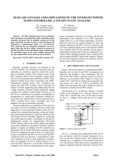
Figure 1 shows <strong>the</strong> scheme <strong>of</strong> a multiconverter IPFC.<br />
Basically, <strong>the</strong> AC side <strong>of</strong> each VSC is connected to its<br />
respective line through a series transformer. The DC<br />
side <strong>of</strong> <strong>the</strong> VSCs share a common circuit. For ease <strong>of</strong><br />
analysis, a two-converter IPFC (Figure 2) whose converters<br />
VSC-1 <strong>and</strong> VSC-2 emulate pure sinusoidal voltage<br />
sources (V C1 <strong>and</strong> V C2 ) will be considered. The<br />
reader will soon notice that such a model can easily be<br />
extended to a multiconverter IPFC scheme.<br />
The injection <strong>of</strong> V C1 on System 1 (Figure 2) usually<br />
results in an exchange <strong>of</strong> P se1 <strong>and</strong> Q se1 between converter<br />
VSC-1 <strong>and</strong> <strong>the</strong> line. Also, for <strong>the</strong> sake <strong>of</strong> analysis,<br />
<strong>the</strong> V C1,2 voltages will be split into its d-q components.<br />
Line 1<br />
Line 2<br />
Series<br />
VSCs<br />
Line 3<br />
VSC-1<br />
VSC-2<br />
VSC-3<br />
Figure 1: Generic scheme <strong>of</strong> an IPFC<br />
The V C1q component has predominant effect on <strong>the</strong><br />
line real <strong>power</strong>, while <strong>the</strong> in-phase component (V C1d )<br />
has over <strong>the</strong> line’s reactive <strong>power</strong>. The reactive <strong>power</strong><br />
exchange Q se1 is supplied by <strong>the</strong> converter itself; however,<br />
<strong>the</strong> presence <strong>of</strong> <strong>the</strong> active <strong>power</strong> component (P se1 )<br />
imposes a dem<strong>and</strong> to <strong>the</strong> DC terminals. Converter VSC-<br />
16th <strong>PSCC</strong>, Glasgow, Scotl<strong>and</strong>, July 14-18, 2008 Page 1
2 is in charge <strong>of</strong> fulfilling this dem<strong>and</strong> through <strong>the</strong><br />
Pse1 + Pse2<br />
= 0 constraint. Unlike VSC-1 (in <strong>the</strong> primary<br />
system) <strong>the</strong> operation <strong>of</strong> VSC-2 (secondary system) has<br />
its freedom degrees reduced; thus, its series voltage V C2<br />
can compensate only partially to its own line. This is<br />
because converter VSC-2 also has <strong>the</strong> task <strong>of</strong> regulating<br />
<strong>the</strong> dc-link voltage. So, <strong>the</strong> P se2 component <strong>of</strong> VSC-2 is<br />
predefined. This imposes a restriction to this line in that<br />
mainly <strong>the</strong> quadrature component <strong>of</strong> V C2 can be specified<br />
to control its <strong>power</strong> <strong>flow</strong>. Under this condition, <strong>the</strong><br />
primary system will have priority over <strong>the</strong> secondary<br />
system in achieving its set-point requirements.<br />
The equivalent sending <strong>and</strong> receiving-end sources in<br />
both AC systems are regarded as stiff. The condition for<br />
which <strong>the</strong> switch CB is closed (i.e. V 11 =V 21 ) also applies<br />
to <strong>the</strong> analysis presented in this section.<br />
System 1<br />
V 11<br />
V 12 V V P<br />
C1<br />
13<br />
V<br />
I 1 14<br />
14<br />
Z 11<br />
(P<br />
CB<br />
se1<br />
+P se2<br />
) = 0<br />
System 2<br />
V P<br />
C2<br />
I 2<br />
24<br />
Z 21<br />
Z 24<br />
V 21<br />
V 22<br />
V 23 V 24<br />
Figure 2: IPFC scheme used in <strong>the</strong> analysis<br />
It will also be assumed that both AC systems have<br />
identical line parameters. Likewise, it is assumed that<br />
each converter injects an ideal sinusoidal waveform<br />
with only its fundamental frequency [8], [9], [13]. The<br />
steady-state <strong>power</strong> balance <strong>of</strong> <strong>the</strong> n number <strong>of</strong> converters<br />
(same number <strong>of</strong> compensated lines) can be represented<br />
by (1):<br />
n<br />
∑<br />
i=<br />
1<br />
P 0<br />
(1)<br />
se _ i<br />
=<br />
As in our case n=2, we will have,<br />
P + = 0<br />
se1<br />
Pse2 (2)<br />
So for each line it can be written,<br />
P<br />
se1<br />
= VC1d<br />
I14d<br />
+ VC1qI14q<br />
(3)<br />
P = V I + V I<br />
(4)<br />
se2<br />
C2d<br />
24d<br />
C2q<br />
From Figure 2, <strong>the</strong> following system equations can<br />
be written:<br />
V12d<br />
= V14d<br />
−VC1<br />
d<br />
− X14I14d<br />
(5a)<br />
V12 q<br />
= V14q<br />
−VC1<br />
q<br />
+ X14I14q<br />
(5b)<br />
V22d<br />
= V24d<br />
−VC<br />
2d<br />
− X<br />
24I<br />
24d<br />
(6a)<br />
V22 q<br />
= V24q<br />
−VC<br />
2q<br />
+ X<br />
24I<br />
24q<br />
(6b)<br />
I14 d<br />
= k1( V11q<br />
−V14q<br />
+ VC1<br />
q<br />
)<br />
(7a)<br />
I14q<br />
= k1( −V11<br />
d<br />
+ V14d<br />
−VC1<br />
d<br />
)<br />
(7b)<br />
I<br />
24 d<br />
= k2<br />
( V21q<br />
−V24q<br />
+ VC<br />
2q<br />
)<br />
(8a)<br />
= k −V<br />
+ V V<br />
(8b)<br />
24q<br />
( )<br />
I<br />
24q<br />
2 21d<br />
24d<br />
−<br />
C 2d<br />
Z 14<br />
where k<br />
= 1<br />
( X + )<br />
,<br />
1<br />
11<br />
X<br />
14<br />
k<br />
= 1<br />
( X<br />
2<br />
21<br />
+ X<br />
24<br />
Equations (2) through (8) allow <strong>the</strong> main parameters<br />
<strong>of</strong> <strong>the</strong> elementary IPFC to be calculated (Figure 2).<br />
Unlike <strong>the</strong> GIPFC case addressed in [13], <strong>the</strong> unknown<br />
variable V C2d will be a function <strong>of</strong> V C1 (specified). Once<br />
computed <strong>the</strong> unknown variables (i.e. <strong>the</strong> d-q components<br />
<strong>of</strong> V 12 , V 22 , I 14 , I 24 <strong>and</strong> V C2d ), <strong>the</strong> <strong>power</strong> <strong>flow</strong> in <strong>the</strong><br />
receiving-end <strong>of</strong> Systems 1 <strong>and</strong> 2, with or without <strong>the</strong><br />
effect <strong>of</strong> <strong>the</strong> series voltage, can be calculated through<br />
(9).<br />
*<br />
S<br />
1<br />
= ( P1<br />
+ jQ1<br />
) = V14<br />
I<br />
(9a)<br />
14<br />
*<br />
S<br />
2<br />
= ( P2<br />
+ jQ<br />
2<br />
) = V24<br />
I<br />
(9b)<br />
24<br />
Note that System 1 will have two independently controlled<br />
variables (i.e. V C1 , θ C1 ). Conversely, System 2<br />
will only have one variable (V C2q ) to be independently<br />
controlled.<br />
3 RESULTS<br />
The results shown in Figures 3 <strong>and</strong> 4 were obtained<br />
using <strong>the</strong> ma<strong>the</strong>matical model developed in Section 2,<br />
in which θ C1 was varied from 0° through 360°. The area<br />
inside <strong>the</strong> circle corresponds to <strong>the</strong> ideal region controlled<br />
by VSC-1, which will be limited by <strong>the</strong> magnitude<br />
<strong>of</strong> V C1 (V max C1 ). The series reactive compensation in<br />
System 2 was set to be null (i.e. V C2q =0), thus, only <strong>the</strong><br />
V C2d component serves as a parameter through which<br />
active <strong>power</strong> is passed from Converter 2 to 1. The way<br />
how VSC-2 compensates to its own line, through its<br />
available reactive compensation, will be shown in Section<br />
3(c).<br />
Q (pu)<br />
0.2<br />
0<br />
-0.2<br />
-0.4<br />
-0.6<br />
P 1<br />
, Q 1<br />
(System 1)<br />
330°<br />
75°<br />
240° 60°<br />
255°<br />
θ C2= 0°<br />
30°<br />
300°<br />
120°<br />
150°<br />
210°<br />
P 2<br />
, Q 2<br />
(System 2)<br />
θ C1 =0°<br />
-0.8<br />
0.4 0.6 0.8 1 1.2 1.4 1.6<br />
P (pu)<br />
Figure 3: P-Q plane (receiving-end) showing <strong>the</strong> operative<br />
region <strong>of</strong> Systems 1 & 2 when V C1 =0.2 pu & V C2d =ƒ(V C1 )<br />
For this particular case, both AC systems were assumed<br />
to have similar transmission angles, i.e. δ 11_14 =<br />
δ 21_24 = -30°. Should <strong>the</strong>se angles be different, maintaining<br />
<strong>the</strong> same V C1 = 0.2 pu, <strong>the</strong> results obtained will be<br />
different. Such a case will also be analysed shortly after.<br />
Notice how <strong>the</strong> <strong>power</strong> <strong>flow</strong> in System 2 is forced to<br />
vary (P 2 ≅0.8pu → 1.2pu, Q 2 ≅-0.6pu → +0.1pu) on<br />
account <strong>of</strong> helping to control P 1 & Q 1 in System 1. For<br />
example, when V C1 =0.2 pu∠60°, with which System 1<br />
increases its active <strong>power</strong> to about P 1 ≅1.4 pu, System 2<br />
(straight line) will need to reduce its active <strong>power</strong> to<br />
)<br />
16th <strong>PSCC</strong>, Glasgow, Scotl<strong>and</strong>, July 14-18, 2008 Page 2
P 2 ≅0.94 pu. As seen in <strong>the</strong>se figures, for <strong>the</strong> full rotation<br />
<strong>of</strong> <strong>the</strong> series angle (θ C1 =0→360°), <strong>the</strong> reactive<br />
<strong>power</strong> Q 2 will experience a broader variation.<br />
The model presented in Section 2 can also be extended<br />
to observe <strong>the</strong> IPFC behavior, mainly <strong>the</strong> degradation<br />
experienced by System 2, when it assists to more<br />
than one line. Figure 4 shows <strong>the</strong> result <strong>of</strong> an IPFC<br />
simultaneously controlling three lines such as those<br />
shown in Figure 1. In this case, <strong>the</strong> primary systems are<br />
constituted by Systems 1 <strong>and</strong> 3, whereas System 2 remains<br />
as <strong>the</strong> secondary (assisting) system. The main<br />
consideration to be done falls again onto eq. (1). In this<br />
case n=3, <strong>the</strong>n (2) will turn into:<br />
P<br />
se1<br />
+ Pse2 + Pse3<br />
= 0<br />
(10)<br />
The rest <strong>of</strong> <strong>the</strong> procedure will be analogous to that<br />
developed while dealing with only 2 series VSCs (same<br />
number <strong>of</strong> compensated lines).<br />
Q (pu)<br />
0.2<br />
0<br />
-0.2<br />
-0.4<br />
-0.6<br />
-0.8<br />
System 1<br />
240°<br />
System 3<br />
30°<br />
0°<br />
75°<br />
0.5 0.6 0.7 0.8 0.9 1 1.1 1.2 1.3 1.4 1.5<br />
Figure 4: (a) Three-converter IPFC, (b) P-Q plane (receiving-end)<br />
<strong>of</strong> Systems 1, 2 <strong>and</strong> 3 when V C1 =0.2 pu∠0→360°,<br />
V C3 =0.1pu∠0→360° & V C2d = ƒ(V C1 , V C3 )<br />
Similarly to <strong>the</strong> conditions imposed in Figure 3, <strong>the</strong> q<br />
component <strong>of</strong> V C2 was set to be null (i.e. no series reactive<br />
compensation was applied to System 2). Notice that<br />
in this case, <strong>the</strong> <strong>power</strong> <strong>flow</strong> over System 2 is significantly<br />
degraded on account <strong>of</strong> <strong>the</strong> help provided to<br />
Systems 1 <strong>and</strong> 3.<br />
a) Bus Voltage Variation due to <strong>the</strong> Series Voltage<br />
Injection – IPFC Primary System<br />
The insertion <strong>of</strong> <strong>the</strong> series voltage in both lines <strong>of</strong> <strong>the</strong><br />
IPFC causes <strong>the</strong> voltages in <strong>the</strong> non-stiff buses to vary.<br />
This variation can trespass some predefined operative<br />
limits <strong>of</strong> <strong>the</strong> bus voltages (e.g. 0.9 pu
In this case, <strong>the</strong> operation <strong>of</strong> <strong>the</strong> series voltage will<br />
be limited to <strong>the</strong> area below <strong>the</strong> shaded areas shown in<br />
Figure 6(b). So, any value <strong>of</strong> V C1 within such areas will<br />
cause overvoltage in <strong>the</strong> operative range <strong>of</strong> bus V 13 . The<br />
same effect will occur in System 2, although this system<br />
can utilise its available reactive compensation (through<br />
<strong>the</strong> V C2q component) to raise or lower to a certain extent<br />
voltage V 23 .<br />
(b) Transmission Angle Effect over <strong>the</strong> Controlled Region<br />
– IPFC Secondary System<br />
It is well established that <strong>the</strong> increase/reduction <strong>of</strong><br />
<strong>the</strong> transmission angle causes <strong>the</strong> line current to also<br />
increase/decrease, if <strong>the</strong> line impedance does not vary.<br />
In this section, <strong>the</strong> effect <strong>of</strong> <strong>the</strong> transmission angle upon<br />
<strong>the</strong> <strong>power</strong> <strong>flow</strong> <strong>of</strong> <strong>the</strong> assisting system will be shown.<br />
Figure 7 shows <strong>the</strong> receiving-end ∆P-∆Q behaviour<br />
corresponding to Line 2. Such results represent <strong>the</strong><br />
incremented <strong>power</strong> around <strong>the</strong> uncompensated case (P 0<br />
& Q 0 ). Generally, <strong>the</strong> total <strong>power</strong> <strong>flow</strong> in both systems,<br />
regarding <strong>the</strong> effect <strong>of</strong> V C1 & V C2 , can be expressed as<br />
P = [ P ∆P]<br />
0 + <strong>and</strong> Q = [ Q ∆Q]<br />
0 + . When δ 21_24 =-30° <strong>the</strong><br />
uncompensated <strong>power</strong> at <strong>the</strong> receiving-end was equal to<br />
P 0 =1.0 <strong>and</strong> Q 0 =-0.2679 pu. When δ 21_24 =0°, <strong>the</strong> reactive<br />
<strong>power</strong> <strong>flow</strong> in <strong>the</strong> receiving-end, ∆Q 2 (Figure 7a), can<br />
be controlled in <strong>the</strong> range ∆Q 2 =±0.4 pu, without affecting<br />
<strong>the</strong> active <strong>power</strong> <strong>flow</strong> at all. An opposite effect<br />
occurs when δ 21_24 = -90°, for which ∆Q 2 =0 <strong>and</strong><br />
∆P 2 =±0.4 pu, though <strong>the</strong> operation under both angles is<br />
in practice remote. Figure 7(b) shows <strong>the</strong> effect <strong>of</strong> <strong>the</strong><br />
transmission angle upon <strong>the</strong> ∆P-∆Q plane for <strong>the</strong> condition<br />
V C2d =0 (similarly to an SSSC – Static Synchronous<br />
Series Compensator) with V C2q being specified. The<br />
positive (Figure 7a), negative (Figure 7b) or even zero<br />
slope <strong>of</strong> <strong>the</strong> control lines can be calculated through (see<br />
also Figure 2):<br />
*<br />
S = V<br />
(10)<br />
I<br />
2 24I<br />
24<br />
24<br />
⎛ V21<br />
− V24<br />
+ V<br />
=<br />
⎜<br />
⎝ jX<br />
C2<br />
⎞<br />
⎟<br />
⎠<br />
(11)<br />
In this case X = (X 21 +X 24 ). So, <strong>the</strong> d-q components <strong>of</strong><br />
I 24 can be written as:<br />
⎛V21q<br />
−V24q<br />
⎞ VC2q<br />
⎛ V<br />
0 C2q ⎞<br />
I =<br />
⎜<br />
⎟ + =<br />
⎜ I +<br />
⎟ (12a)<br />
24d<br />
d<br />
⎝ X ⎠ X ⎝ X ⎠<br />
⎛ V21d<br />
− V24d<br />
⎞ VC2d<br />
⎛ 0 VC2d<br />
⎞<br />
I = ⎜−<br />
⎟ − = ⎜ I − ⎟ (12b)<br />
24q<br />
q<br />
⎝ X ⎠ X ⎝ X ⎠<br />
Substituting (12) into (10) yields,<br />
0<br />
0<br />
⎛ VC2q<br />
V ⎞<br />
C2d 0<br />
P2 ( V24d<br />
I<br />
d<br />
V24qI<br />
q<br />
) ⎜V24d<br />
V24q<br />
= ( P + ∆P2<br />
)<br />
X X<br />
⎟ (13a)<br />
= + + −<br />
⎝<br />
⎠<br />
0<br />
0<br />
⎛ VC2q<br />
V ⎞<br />
C2d 0<br />
Q2 ( V24qI<br />
d<br />
V24d<br />
I<br />
q<br />
) V24q<br />
V24d<br />
= ( Q + ∆Q2<br />
)<br />
(13b)<br />
= − +<br />
⎜ +<br />
X X<br />
⎟<br />
⎝<br />
⎠<br />
Writing ∆P 2 <strong>and</strong> ∆Q 2 in a matrix form, we obtain:<br />
⎡ ∆P2<br />
⎤<br />
⎢ ⎥ =<br />
⎣∆Q2<br />
⎦<br />
1<br />
X<br />
⎡V<br />
⎢<br />
⎣V<br />
24d<br />
24q<br />
−V<br />
V<br />
24q<br />
24d<br />
⎤⎡V<br />
⎥⎢<br />
⎦⎣V<br />
C2q<br />
C2d<br />
⎤<br />
⎥<br />
⎦<br />
(14)<br />
If V C2q =0 <strong>and</strong> as V C2d is a function <strong>of</strong> V C1<br />
(V C1 =0.2pu∠0°→360°) <strong>the</strong>n:<br />
∆P V<br />
2 24q<br />
= −<br />
(15a)<br />
∆Q2<br />
V24d<br />
V24d<br />
∆Q2 = − ∆P<br />
(15b)<br />
2<br />
V<br />
24q<br />
Which draw <strong>the</strong> positive slopes <strong>of</strong> <strong>the</strong> control lines<br />
shown in Figure 7(a).<br />
0.4<br />
0.2<br />
∆Q 0<br />
-0.2<br />
δ 21−24<br />
= 0°<br />
System 1<br />
V C1<br />
=0.2 pu (0° to 360°)<br />
-0.4<br />
-0.4 -0.2 0 0.2 0.4<br />
P<br />
0.4<br />
0.2<br />
∆Q 0<br />
-0.2<br />
−30°<br />
δ 21−24<br />
= 0°<br />
− 60°<br />
∆<br />
(a)<br />
−30°<br />
−60°<br />
δ 21−24<br />
= −90°<br />
System 2<br />
− 90°<br />
System 2<br />
-0.4<br />
-0.4 -0.2 0 0.2 0.4<br />
∆ P<br />
Figure 7: Power <strong>flow</strong> in Line 2 (receiving-end) for several<br />
values <strong>of</strong> δ 11_14 : (a) V C2q =0 <strong>and</strong> V C2d =ƒ(V C1 ), positive slope;<br />
(b) V C2d =0 <strong>and</strong> V C2q =0.2 pu, negative slope<br />
(b)<br />
If V C2d = 0 <strong>and</strong> as V C2q =0.2 pu, <strong>the</strong>n (14) becomes:<br />
∆P2<br />
V24d<br />
= −<br />
(16a)<br />
∆Q V<br />
2<br />
V<br />
24q<br />
24q<br />
∆Q<br />
2<br />
= ∆P<br />
(16b)<br />
2<br />
V24d<br />
Which draw <strong>the</strong> positive slopes <strong>of</strong> <strong>the</strong> control lines<br />
shown in Figure 7(b).<br />
c) Control Area <strong>of</strong> <strong>the</strong> IPFC Secondary System<br />
Since <strong>the</strong> primary system <strong>of</strong> <strong>the</strong> IPFC behaves similarly<br />
to a line compensated through a UPFC, its control<br />
area in <strong>the</strong> P-Q plane will correspond to that shown in<br />
Figure 3. Due to <strong>the</strong> inherent restrictions <strong>of</strong> <strong>the</strong> secondary<br />
system, each value <strong>of</strong> V C2q will create parallel line<br />
leftwards <strong>of</strong> <strong>the</strong> M-N line (if V C2q is inductive) or rightwards<br />
<strong>of</strong> it (if V C2q is capacitive); thus, giving place to<br />
16th <strong>PSCC</strong>, Glasgow, Scotl<strong>and</strong>, July 14-18, 2008 Page 4
<strong>the</strong> skewed area shown in Figure 8. The M-N line<br />
shown in this figure has no series reactive compensation<br />
(i.e. V C2q = 0).<br />
Apparently, <strong>the</strong> secondary system might have a bigger<br />
control area than <strong>the</strong> primary system. However,<br />
because both converters are rated with <strong>the</strong> same capacity,<br />
this control area will be basically limited to <strong>the</strong><br />
same circular area as that <strong>of</strong> Line 1. For example, if we<br />
consider point B in Figure 8, which is out <strong>of</strong> <strong>the</strong> circular<br />
area, converter VSC-2 would not be able to fully accomplish<br />
its compensation function on both lines. This<br />
can be verified by comparing <strong>the</strong> boundaries <strong>of</strong> <strong>the</strong><br />
controlled regions, which should be equal.<br />
For any point inside <strong>the</strong> circle, it can be verified that:<br />
max<br />
∆ = ( ∆P<br />
+ j∆Q<br />
) 0.4 pu.<br />
S1 1 1<br />
≤<br />
As for point B, outside <strong>the</strong> circle, <strong>the</strong> pu value will<br />
be:<br />
B<br />
∆S<br />
2<br />
= ∆P2<br />
+ ∆Q<br />
2<br />
2<br />
2<br />
=<br />
2<br />
0.2 + ( −<br />
0.4)<br />
2<br />
= 0.447 pu<br />
This value is greater than <strong>the</strong> maximum value corresponding<br />
to that drawn by converter VSC-1<br />
B max<br />
B<br />
( ∆ S2 > ∆S1<br />
), thus, ∆ S 2<br />
can not be considered<br />
as an operative point <strong>of</strong> System 2.<br />
0.6<br />
0.4<br />
0.2<br />
C<br />
V C2q<br />
(ind.)<br />
M<br />
V C2q<br />
(cap.)<br />
d) Transmission Angle Effect upon <strong>the</strong> Converters<br />
This section shows <strong>the</strong> steady-state response <strong>of</strong> <strong>the</strong><br />
series converters when <strong>the</strong> transmission angle is simultaneously<br />
varied. This analysis resulted also from <strong>the</strong><br />
model developed in Section 2. In order to observe <strong>the</strong><br />
effect <strong>of</strong> transmission angle, <strong>the</strong> series voltage in both<br />
systems were kept constant at V C1 =0.2 pu ∠0→360°<br />
<strong>and</strong> V C2q =0. Once computed <strong>the</strong> line current in each<br />
line, eqs. (19a) <strong>and</strong> (19b) were used to compute P se <strong>and</strong><br />
Q se in also each converter.<br />
*<br />
S<br />
se1<br />
= ( Pse1<br />
+ jQse1<br />
) = VC1I<br />
(17)<br />
L1<br />
V11<br />
−V14<br />
+ VC1<br />
I<br />
L1<br />
= (18)<br />
jX<br />
1<br />
from which it can be obtained:<br />
V<br />
C1<br />
Pse1<br />
= [ V11<br />
sin ( δ11<br />
− θ<br />
C1<br />
) − V14<br />
sin ( δ14<br />
− θ<br />
C1<br />
)]<br />
(19a)<br />
X<br />
1<br />
VC1<br />
Q<br />
se1<br />
= [ V11cos( δ11<br />
- θC1<br />
) −V14cos( δ14<br />
- θC1<br />
) + VC1<br />
] (19b)<br />
X<br />
1<br />
Figure 9(a) shows <strong>the</strong> case when <strong>the</strong> transmission<br />
angle in System 1 is varied (δ 11_14 = -10°, -20°, -30°)<br />
while that <strong>of</strong> System 2 was kept constant at δ 21-24 = -<br />
30°.<br />
0.3<br />
0.2<br />
0.1<br />
Q se<br />
VSC - 1<br />
-10°<br />
-20°<br />
-30°<br />
∆ Q<br />
0<br />
System 1<br />
0<br />
-0.2<br />
System 2<br />
-0.1<br />
VSC - 2<br />
-0.2 -0.1 0 0.1 0.2<br />
-0.4<br />
N<br />
-0.6<br />
-0.6 -0.4 -0.2 0 0.2 0.4 0.6<br />
∆ P<br />
Figure 8: Ideal control region (IPFC Secondary system) at<br />
<strong>the</strong> receiving-end: V C2q =0→±0.2 pu, V C2p =ƒ(V C1 ) e<br />
V C1 =0.2∠0→360°<br />
Actually, as V C2q increases from V C2q =0→±0.2pu (inductive<br />
or capacitive mode) <strong>the</strong> V C2d component will<br />
decrease. Similarly to Section 3(b), <strong>the</strong> ∆P-∆Q controlled<br />
region shown in this figure does not correspond<br />
to <strong>the</strong> capacity <strong>of</strong> <strong>the</strong> converters, but to <strong>the</strong> incremented<br />
<strong>power</strong> around P 0 &Q 0 in <strong>the</strong> receiving-end. Also, as V C2q<br />
is increased (i.e. displacing <strong>the</strong> M-N line leftwards or<br />
rightwards) <strong>the</strong> V C2d component will decrease. This<br />
occurs so as to maintain <strong>the</strong> capacity <strong>of</strong> converter VSC-<br />
2, which should not be trespassed. Should <strong>the</strong> M-N line<br />
be displaced even fur<strong>the</strong>r, for example reaching point C,<br />
both converters will be operating as independent SSSCs<br />
with angles 75° (inductive mode <strong>of</strong> V C2q ) or 255° (capacitive<br />
mode <strong>of</strong> V C2q ). Thus, <strong>the</strong> active <strong>power</strong> exchange<br />
between <strong>the</strong> converters will be zero.<br />
B<br />
0.6<br />
0.5<br />
0.4<br />
0.3<br />
Q se 0.2<br />
0.1<br />
0<br />
-0.1<br />
-0.2<br />
VSC - 2<br />
P se<br />
(a)<br />
VSC - 1<br />
-10°<br />
-0.2 -0.1 0 0.1 0.2<br />
P se<br />
-20°<br />
-30°<br />
(b)<br />
Figure 9: Control region <strong>of</strong> converters VSC-1 & VSC-2<br />
when V C1 =0.2 pu ∠0→360° <strong>and</strong> V C2q =0: (a) δ 11_14 = -10°, -<br />
20°, -30° <strong>and</strong> δ 21_24 = -30°, (b) δ 11_14 = -30° <strong>and</strong> δ 21_24 = -10°,<br />
-20°, -30°<br />
It can be seen that <strong>the</strong> active <strong>power</strong> dem<strong>and</strong> P se1 increases<br />
proportionally to δ 11_14 . Likewise, P se2 varies<br />
16th <strong>PSCC</strong>, Glasgow, Scotl<strong>and</strong>, July 14-18, 2008 Page 5
according to δ 11_14 (blue curves) as it has to fulfil <strong>the</strong><br />
dem<strong>and</strong> <strong>of</strong> P se1 . The reactive <strong>power</strong> Q se2 (at VSC-2)<br />
shows a less variation compared to that experienced by<br />
P se2 .<br />
Once reversed this condition, that is, <strong>the</strong> transmission<br />
angle in System 2 is varied (δ 21_24 = -10°, -20°, -<br />
30°) while <strong>the</strong> angle <strong>of</strong> System 1 is kept constant (δ 11_14<br />
= -30°), <strong>the</strong> reactive <strong>power</strong> Q se2 (blue curves) becomes<br />
highly affected (Figure 9b). Conversely, <strong>the</strong> real <strong>power</strong><br />
<strong>of</strong> VSC-2 (P se2 ) operates nearly in <strong>the</strong> same range (-0.2,<br />
+0.2 pu). Obviously, <strong>the</strong> variation <strong>of</strong> δ 21_24 will be also<br />
reflected in <strong>the</strong> variation <strong>of</strong> <strong>the</strong> <strong>power</strong> <strong>flow</strong> (P 2 ) in System<br />
2.<br />
4 CONCLUSIONS<br />
This paper showed <strong>the</strong> main attributes <strong>and</strong> dis<strong>advantages</strong><br />
characterising <strong>the</strong> operation <strong>of</strong> <strong>the</strong> IPFC whilst<br />
controlling <strong>the</strong> <strong>power</strong> <strong>flow</strong> in multiline systems.<br />
Issues like <strong>the</strong> <strong>power</strong> <strong>flow</strong> degradation in <strong>the</strong> system<br />
termed as secondary <strong>and</strong> <strong>the</strong> bus voltage variation in<br />
both systems on account <strong>of</strong> helping to manipulate <strong>the</strong><br />
series voltage in <strong>the</strong> primary system(s), were also addressed.<br />
It was also shown that maintaining <strong>the</strong> bus<br />
voltage within certain technical limits, it was <strong>the</strong> case <strong>of</strong><br />
voltage V 13 , imposes some restrictions to <strong>the</strong> operative<br />
region <strong>of</strong> <strong>the</strong> series voltage (V C1 ). Some o<strong>the</strong>r steadystate<br />
operative conditions such as <strong>the</strong> variation <strong>of</strong> <strong>the</strong><br />
transmission angle <strong>and</strong> its effect over both systems were<br />
also analysed in <strong>the</strong> paper.<br />
Despite <strong>the</strong> above mentioned drawbacks <strong>the</strong> IPFC,<br />
even in its simplest form (i.e. with only two series converters)<br />
can be very attractive <strong>and</strong> useful for relieving<br />
congested systems.<br />
REFERENCES<br />
[1] B. Fardanesh, B. Shperling, E. Uzunovic, S.<br />
Zelingher, “Multi-converter FACTS Devices: <strong>the</strong><br />
Generalized Unified Power Flow Controller<br />
(GUPFC),” in Proc. IEEE Power Engineering Society<br />
Summer Meeting, v. 2, 16-20 July 2000, pp.<br />
1020-1025.<br />
[2] V. Diez-Valencia, U.D. Annakkage, A.M. Gole, P.<br />
Demchenko, D. Jacobson, “Interline Power Flow<br />
Controller (IPFC) Steady State Operation,” in<br />
Proc. Canadian Conference on Electrical <strong>and</strong><br />
Computer Engineering, IEEE CCECE 2002, v. 1,<br />
2002, pp. 280-284.<br />
[3] X. Wei, J.H. Chow, B. Fardanesh, A.A. Edris, “A<br />
Dispatch Strategy for an Interline Power Flow<br />
Controller Operating at Rated Capacity.” In: Proc.<br />
PSCE 2004 – Power Systems Conference & Exposition,<br />
IEEE PES, New York, Oct. 10-13, 2004.<br />
[4] J. Sun, L. Hopkins, B. Shperling, B. Fardanesh, M.<br />
Graham, M. Parisi, S. Macdonald, S. Bhattacharya,<br />
S. Berkowitz, A.A. Edris, “Operating Characteristics<br />
<strong>of</strong> <strong>the</strong> Convertible Static Compensator on <strong>the</strong><br />
345 kV Network,” in Proc. PSCE 2004 – Power<br />
Systems Conference & Exposition, IEEE PES, New<br />
York, v. 2, Oct. 10-13, 2004, pp. 732-738.<br />
[5] B. Fardanesh, “Optimal Utilization, Sizing, <strong>and</strong><br />
Steady-State Performance Comparison <strong>of</strong> Multiconverter<br />
VSC-Based FACTS Controllers,” IEEE<br />
Transactions on Power Delivery, Vol. 19, No. 3,<br />
pp. 1321-1327, July, 2004.<br />
[6] X-P. Zhang, "Multiterminal Voltage-Sourced Converter-Based<br />
HVDC Models for Power Flow<br />
Analysis," IEEE Transactions on Power Systems,<br />
Vol. 19, No. 4, pp. 1877-1884, Nov. 2004.<br />
[7] X-P. Zhang, E. H<strong>and</strong>schin, M. Yao, “Modeling <strong>of</strong><br />
<strong>the</strong> Generalized Unified Power Flow Controller<br />
(GUPFC) in a Nonlinear Interior Point OPF,”<br />
IEEE Transactions on Power Systems, Vol. 16,<br />
No. 3, pp. 367-373, Aug. 2001.<br />
[8] R.L. Vasquez-Arnez, L.C. Zanetta Jr., “Operational<br />
Analysis <strong>and</strong> Limitations <strong>of</strong> <strong>the</strong> VSI-Based Multi-<br />
Line FACTS Controllers,” SBA Control & Automation<br />
Journal, Vol. 17, No. 2, Apr./June 2006, ISSN<br />
0103-1759, pp. 167-176.<br />
[9] Y. Zhang, C. Chen, Y. Zhang, “A Novel Power<br />
Injection Model <strong>of</strong> IPFC for Power Flow Analysis<br />
Inclusive <strong>of</strong> Practical Constraints,” IEEE Transactions<br />
on Power Systems, Vol. 21, No. 4, pp. 1550 –<br />
1556, Nov. 2006.<br />
[10] L. Gyugyi, K.K. Sen, C.D. Schauder, “The Interline<br />
Power Flow Controller Concept: A New Approach<br />
to Power Flow Management in Transmission<br />
System,” IEEE Trans. Power Delivery, Vol.<br />
14, no.3, pp. 1115-1123, 1999.<br />
[11] S. Salem, V. K. Sood, “Simulation <strong>and</strong> Controller<br />
Design <strong>of</strong> an Interline Power Flow Controller in<br />
EMTP RV,” in Proc. International Conference on<br />
Power Systems Transients (IPST'07), Lyon, June<br />
4-7, 2007.<br />
[12] S. Sankar, S. Ramareddy, “Simulation <strong>and</strong> Implementation<br />
<strong>of</strong> Interline Power Flow Controller System,”<br />
International Journal <strong>of</strong> Applied Engineering<br />
Research, Vol. 2, No. 4, 2007, pp. 557–568.<br />
[13] R.L. Vasquez-Arnez, L.C. Zanetta Jr., “A New<br />
Approach for Modeling <strong>the</strong> Multi-Line VSC-Based<br />
FACTS Controllers <strong>and</strong> <strong>the</strong>ir Operational Constraints,”<br />
IEEE Transactions on Power Delivery,<br />
Vol. 23, No. 1, Jan. 2008. pp. 457-464.<br />
[14] N.G. Hingorani, L. Gyugyi, “Underst<strong>and</strong>ing<br />
FACTS: Concepts <strong>and</strong> Technology <strong>of</strong> Flexible AC<br />
Transmission Systems.” New York, IEEE Press,<br />
2000.<br />
16th <strong>PSCC</strong>, Glasgow, Scotl<strong>and</strong>, July 14-18, 2008 Page 6