Implementing Qubits with Superconducting Integrated Circuits

Quantum Information Processing, Vol. 3, Nos. 1–5, October 2004 (© 2004) 

Implementing Qubits with Superconducting 

Integrated Circuits 

Michel H. Devoret 1,4 and John M. Martinis 2,3 

Received March 2, 2004; accepted June 2, 2004 

Superconducting qubits are solid state electrical circuits fabricated using techniques 

borrowed from conventional integrated circuits. They are based on the 

Josephson tunnel junction, the only non-dissipative, strongly non-linear circuit element 

available at low temperature. In contrast to microscopic entities such as 

spins or atoms, they tend to be well coupled to other circuits, which make them 

appealling from the point of view of readout and gate implementation. Very 

recently, new designs of superconducting qubits based on multi-junction circuits 

have solved the problem of isolation from unwanted extrinsic electromagnetic perturbations. 

We discuss in this review how qubit decoherence is affected by the 

intrinsic noise of the junction and what can be done to improve it. 

KEY WORDS: Quantum information; quantum computation; superconducting 

devices; Josephson tunnel junctions; integrated circuits. 

PACS: 03.67.−a, 03.65.Yz, 85.25.−j, 85.35.Gv. 

1. INTRODUCTION 

1.1. The Problem of Implementing a Quantum Computer 

The theory of information has been revolutionized by the discovery 

that quantum algorithms can run exponentially faster than their classical 

counterparts, and by the invention of quantum error-correction protocols. 

(1) These fundamental breakthroughs have lead scientists and engineers 

to imagine building entirely novel types of information processors. 

However, the construction of a computer exploiting quantum—rather than 

1 Applied Physics Department, Yale University, New Haven, CT 06520, USA. 

2 National Institute of Standards and Technology, Boulder, CO 80305, USA. 

3 Present address: Physics Department, University of California, Santa Barbara, CA 93106, 

USA. 

4 To whom correspondence should be addressed. E-mail: michel.devoret@yale.edu 

163 

1570-0755/04/1000-0163/0 © 2004 Springer Science+Business Media, Inc.

164 Devoret and Martinis 

classical—principles represents a formidable scientific and technological 

challenge. While quantum bits must be strongly inter-coupled by gates 

to perform quantum computation, they must at the same time be completely 

decoupled from external influences, except during the write, control 

and readout phases when information must flow freely in and out of the 

machine. This difficulty does not exist for the classical bits of an ordinary 

computer, which each follow strongly irreversible dynamics that damp the 

noise of the environment. 

Most proposals for implementing a quantum computer have been 

based on qubits constructed from microscopic degrees of freedom: spin of 

either electrons or nuclei, transition dipoles of either atoms or ions in vacuum. 

These degrees of freedom are naturally very well isolated from their 

environment, and hence decohere very slowly. The main challenge of these 

implementations is enhancing the inter-qubit coupling to the level required 

for fast gate operations without introducing decoherence from parasitic 

environmental modes and noise. 

In this review, we will discuss a radically different experimental 

approach based on “quantum integrated circuits.” Here, qubits are constructed 

from collective electrodynamic modes of macroscopic electrical 

elements, rather than microscopic degrees of freedom. An advantage of 

this approach is that these qubits have intrinsically large electromagnetic 

cross-sections, which implies they may be easily coupled together in complex 

topologies via simple linear electrical elements like capacitors, inductors, 

and transmission lines. However, strong coupling also presents a 

related challenge: is it possible to isolate these electrodynamic qubits from 

ambient parasitic noise while retaining efficient communication channels 

for the write, control, and read operations? The main purpose of this article 

is to review the considerable progress that has been made in the past 

few years towards this goal, and to explain how new ideas about methodology 

and materials are likely to improve coherence to the threshold 

needed for quantum error correction. 

1.2. Caveats 

Before starting our discussion, we must warn the reader that this 

review is atypical in that it is neither historical nor exhaustive. Some 

important works have not been included or are only partially covered. On 

the other hand, the reader may feel we too frequently cite our own work, 

but we wanted to base our speculations on experiments whose details we 

fully understand. We have on purpose narrowed our focus: we adopt the 

point of view of an engineer trying to determine the best strategy for 

building a reliable machine given certain design criteria. This approach

Implementing Qubits with Superconducting Integrated Circuits 165 

obviously runs the risk of presenting a biased and even incorrect account 

of recent scientific results, since the optimization of a complex system is 

always an intricate process with both hidden passageways and dead-ends. 

We hope nevertheless that the following sections will at least stimulate discussions 

on how to harness the physics of quantum integrated circuits into 

a mature quantum information processing technology. 

2. BASIC FEATURES OF QUANTUM INTEGRATED CIRCUITS 

2.1. Ultra-low Dissipation: Superconductivity 

For an integrated circuit to behave quantum mechanically, the first 

requirement is the absence of dissipation. More specifically, all metallic 

parts need to be made out of a material that has zero resistance at the 

qubit operating temperature and at the qubit transition frequency. This is 

essential in order for electronic signals to be carried from one part of the 

chip to another without energy loss—a necessary (but not sufficient) condition 

for the preservation of quantum coherence. Low temperature superconductors 

such as aluminium or niobium are ideal for this task. (2) For 

this reason, quantum integrated circuit implementations have been nicknamed 

“superconducting qubits” 1 . 

2.2. Ultra-low Noise: Low Temperature 

The degrees of freedom of the quantum integrated circuit must be 

cooled to temperatures where the typical energy kT of thermal fluctuations 

is much less that the energy quantum ω 01 associated with the transition 

between the states |qubit = 0〉 and |qubit = 1〉. For reasons which 

will become clear in subsequent sections, this frequency for superconducting 

qubits is in the 5–20 GHz range and therefore, the operating temperature 

T must be around 20 mK (recall that 1 K corresponds to about 

20 GHz). These temperatures may be readily obtained by cooling the chip 

with a dilution refrigerator. Perhaps more importantly though, the “electromagnetic 

temperature” of the wires of the control and readout ports 

connected to the chip must also be cooled to these low temperatures, 

which requires careful electromagnetic filtering. Note that electromagnetic 

1 In principle, other condensed phases of electrons, such as high-T c superconductivity or the 

quantum Hall effect, both integer and fractional, are possible and would also lead to quantum 

integrated circuits of the general type discussed here. We do not pursue this subject further 

than this note, however, because dissipation in these new phases is, by far, not as well 

understood as in low-T c superconductivity.


(a) 

SUPERCONDUCTING 

BOTTOM 

ELECTRODE 

SUPERCONDUCTING 

TOP ELECTRODE 

TUNNEL OXIDE 

LAYER 

(b) 

I 0 

C J 

Fig. 1. (a) Josephson tunnel junction made with two superconducting thin films; (b) 

Schematic representation of a Josephson tunnel junction. The irreducible Josephson element 

is represented by a cross. 

damping mechanisms are usually stronger at low temperatures than those 

originating from electron–phonon coupling. The techniques (3) and requirements 

(4) for ultra-low noise filtering have been known for about 20 years. 

From the requirements kT ≪ ω 01 and ω 01 ≪ , where is the energy 

gap of the superconducting material, one must use superconducting materials 

with a transition temperature greater than about 1 K. 

2.3. Non-linear, Non-dissipative Elements: Tunnel Junctions 

Quantum signal processing cannot be performed using only purely 

linear components. In quantum circuits, however, the non-linear elements 

must obey the additional requirement of being non-dissipative. Elements 

like PIN diodes or CMOS transistors are thus forbidden, even if they 

could be operated at ultra-low temperatures. 

There is only one electronic element that is both non-linear and nondissipative 

at arbitrarily low temperature: the superconducting tunnel junction 

2 (also known as a Josephson tunnel junction (5) ). As illustrated in 

Fig. 1, this circuit element consists of a sandwich of two superconducting 

thin films separated by an insulating layer that is thin enough (typically 

∼1 nm) to allow tunneling of discrete charges through the barrier. In later 

2 A very short superconducting weak link (see for instance Ref. 6) is a also a possible candidate, 

provided the Andreev levels would be sufficiently separated. Since we have too few 

experimental evidence for quantum effects involving this device, we do not discuss this otherwise 

important matter further.


sections we will describe how the tunneling of Cooper pairs creates an 

inductive path with strong non-linearity, thus creating energy levels suitable 

for a qubit. The tunnel barrier is typically fabricated from oxidation 

of the superconducting metal. This results in a reliable barrier since the 

oxidation process is self-terminating. (7) The materials properties of amorphous 

aluminum oxide, alumina, make it an attractive tunnel insulating 

layer. In part because of its well-behaved oxide, aluminum is the material 

from which good quality tunnel junctions are most easily fabricated, and it 

is often said that aluminium is to superconducting quantum circuits what 

silicon is to conventional MOSFET circuits. Although the Josephson effect 

is a subtle physical effect involving a combination of tunneling and superconductivity, 

the junction fabrication process is relatively straightforward. 

2.4. Design and Fabrication of Quantum Integrated Circuits 

Superconducting junctions and wires are fabricated using techniques 

borrowed from conventional integrated circuits 3 . Quantum circuits are 

typically made on silicon wafers using optical or electron-beam lithography 

and thin film deposition. They present themselves as a set of micronsize 

or sub-micron-size circuit elements (tunnel junctions, capacitors, and 

inductors) connected by wires or transmission lines. The size of the chip 

and elements are such that, to a large extent, the electrodynamics of the 

circuit can be analyzed using simple transmission line equations or even 

a lumped element approximation. Contact to the chip is made by wires 

bonded to mm-size metallic pads. The circuit can be designed using conventional 

layout and classical simulation programs. 

Thus, many of the design concepts and tools of conventional semiconductor 

electronics can be directly applied to quantum circuits. Nevertheless, 

there are still important differences between conventional and 

quantum circuits at the conceptual level. 

2.5. Integrated Circuits that Obey Macroscopic Quantum Mechanics 

At the conceptual level, conventional and quantum circuits differ in 

that, in the former, the collective electronic degrees of freedom such as 

currents and voltages are classical variables, whereas in the latter, these 

degrees of freedom must be treated by quantum operators which do 

not necessarily commute. A more concrete way of presenting this rather 

3 It is worth mentioning that chips with tens of thousands of junctions have been successfully 

fabricated for the voltage standard and for the Josephson signal processors, which are only 

exploiting the speed of Josephson elements, not their macroscopic quantum properties.


abstract difference is to say that a typical electrical quantity, such as the 

charge on the plates of a capacitor, can be thought of as a simple number 

is conventional circuits, whereas in quantum circuits, the charge on 

the capacitor must be represented by a wave function giving the probability 

amplitude of all charge configurations. For example, the charge on 

the capacitor can be in a superposition of states where the charge is both 

positive and negative at the same time. Similarly the current in a loop 

might be flowing in two opposite directions at the same time. These situations 

have originally been nicknamed “macroscopic quantum coherence 

effects” by Tony Leggett (8) to emphasize that quantum integrated circuits 

are displaying phenomena involving the collective behavior of many particles, 

which are in contrast to the usual quantum effects associated with 

microscopic particles such as electrons, nuclei or molecules 4 . 

2.6. DiVicenzo Criteria 

We conclude this section by briefly mentioning how quantum integrated 

circuits satisfy the so-called DiVicenzo criteria for the implementation 

of quantum computation. (9) The non-linearity of tunnel junctions 

is the key property ensuring that non-equidistant level subsystems can be 

implemented (criterion #1: qubit existence). As in many other implementations, 

initialization is made possible (criterion #2: qubit reset) by the 

use of low temperature. Absence of dissipation in superconductors is one 

of the key factors in the quantum coherence of the system (criterion #3: 

qubit coherence). Finally, gate operation and readout (criteria #4 and #5) 

are easily implemented here since electrical signals confined to and traveling 

along wires constitute very efficient coupling methods. 

3. THE SIMPLEST QUANTUM CIRCUIT 

3.1. Quantum LC Oscillator 

We consider first the simplest example of a quantum integrated circuit, 

the LC oscillator. This circuit is shown in Fig. 2, and consists 

of an inductor L connected to a capacitor C, all metallic parts being 

superconducting. This simple circuit is the lumped-element version of a 

superconducting cavity or a transmission line resonator (for instance, the 

link between cavity resonators and LC circuits is elegantly discussed by 

4 These microscopic effects determine also the properties of materials, and explain phenomena 

such as superconductivity and the Josephson effect itself. Both classical and quantum circuits 

share this bottom layer of microscopic quantum mechanics.


C 

L 

Fig. 2. 

Lumped element model for an electromagnetic resonator: LC oscillator. 

Feynman (10) ). The equations of motion of the LC circuit are those of an 

harmonic oscillator. It is convenient to take the position coordinate as 

being the flux in the inductor, while the role of conjugate momentum 

is played by the charge Q on the capacitor playing the role of its conjugate 

momentum. The variables and Q have to be treated as canonically 

conjugate quantum operators that obey [, Q] = i. The hamiltonian of 

the circuit is H = (1/2) 2 /L + (1/2)Q 2 /C, which can be equivalently written 

as H = ω 0 (n + (1/2)) where n is the number operator for photons in 

the resonator and ω 0 =1/ √ LC is the resonance frequency of the oscillator. 

It is important to note that the parameters of the circuit hamiltonian are 

not fundamental constants of Nature. They are engineered quantities with 

a large range of possible values which can be modified easily by changing 

the dimensions of elements, a standard lithography operation. It is 

in this sense, in our opinion, that the system is unambiguously “macroscopic”. 

The other important combination of the parameters L and C is 

the characteristic impedance Z = √ L/C of the circuit. When we combine 

this impedance with the residual resistance of the circuit and/or its radiation 

losses, both of which we can lump into a resistance R, we obtain 

the quality factor of the oscillation: Q=Z/R. The theory of the harmonic 

oscillator shows that a quantum superposition of ground state and first 

excited state decays on a time scale given by 1/RC. This last equality illustrates 

the general link between a classical measure of dissipation and the 

upper limit of the quantum coherence time. 

3.2. Practical Considerations 

In practice, the circuit shown in Fig. 2 may be fabricated using planar 

components with lateral dimensions around 10 µm, giving values of L 

and C approximately 0.1 nH and 1 pF, respectively, and yielding ω 0 /2π ≃ 

16 GHz and Z 0 = 10 . If we use aluminium, a good BCS superconductor 

with transition temperature of 1.1 K and a gap /e≃ 200 µV , dissipation 

from the breaking of Cooper pairs will begin at frequencies greater 

than 2/h ≃ 100 GHz. The residual resistivity of a BCS superconductor 

decreases exponentially with the inverse of temperature and linearly


with frequency, as shown by the Mattis-Bardeen (MB) formula ρ (ω) ∼ 

ρ 0 (ω/k B T)exp (−/k B T ), (11) where ρ 0 is the resistivity of the metal in 

the normal state (we are treating here the case of the so-called “dirty” 

superconductor, (12) which is well adapted to thin film systems). According 

to MB, the intrinsic losses of the superconductor at the temperature 

and frequency (typically 20 mK and 20 GHz) associated with qubit dynamics 

can be safely neglected. However, we must warn the reader that the 

intrisinsic losses in the superconducting material do not exhaust, by far, 

sources of dissipation, even if very high quality factors have been demonstrated 

in superconducting cavity experiments. (13) 

3.3. Matching to the Vacuum Impedance: A Useful Feature, not a Bug 

Although the intrisinsic dissipation of superconducting circuits can be 

made very small, losses are in general governed by the coupling of the 

circuit with the electromagnetic environment that is present in the forms 

of write, control and readout lines. These lines (which we also refer to 

as ports) have a characteristic propagation impedance Z c ≃ 50 , which 

is constrained to be a fraction of the impedance of the vacuum Z vac = 

377 . It is thus easy to see that our LC circuit, with a characteristic 

impedance of Z 0 = 10 , tends to be rather well impedance-matched to 

any pair of leads. This circumstance occurs very frequently in circuits, and 

almost never in microscopic systems such as atoms which interact very 

weakly with electromagnetic radiation 5 . Matching to Z vac is a useful feature 

because it allows strong coupling for writing, reading, and logic operations. 

As we mentioned earlier, the challenge with quantum circuits is to 

isolate them from parasitic degrees of freedom. The major task of this 

review is to explain how this has been achieved so far and what level of 

isolation is attainable. 

3.4. The Consequences of being Macroscopic 

While our example shows that quantum circuits can be mass-produced 

by standard micro-fabrication techniques and that their parameters 

can be easily engineered to reach some optimal condition, it also points 

out evident drawbacks of being “macroscopic” for qubits. 

5 The impedance of an atom can be crudely seen as being given by the impedance quantum 

R K = h/e 2 . We live in a universe where the ratio Z vac /2R K , also known as the fine structure 

constant 1/137.0, is a small number.


The engineered quantities L and C can be written as 

L = L stat + L(t), 

C = C stat + C(t). 

(1) 

(a) The first term on the right-hand side denotes the static part of the 

parameter. It has statistical variations: unlike atoms whose transition frequencies 

in isolation are so reproducible that they are the basis of atomic 

clocks, circuits will always be subject to parameter variations from one 

fabrication batch to another. Thus prior to any operation using the circuit, 

the transition frequencies and coupling strength will have to be determined 

by “diagnostic” sequences and then taken into account in the algorithms. 

(b) The second term on the right-hand side denotes the time-dependent 

fluctuations of the parameter. It describes noise due to residual 

material defects moving in the material of the substrate or in the material 

of the circuit elements themselves. This noise can affect for instance 

the dielectric constant of a capacitor. The low frequency components of 

the noise will make the resonance frequency wobble and contribute to the 

dephasing of the oscillation. Furthermore, the frequency component of the 

noise at the transition frequency of the resonator will induce transitions 

between states and will therefore contribute to the energy relaxation. 

Let us stress that statistical variations and noise are not problems 

affecting superconducting qubit parameters only. For instance when several 

atoms or ions are put together in microcavities for gate operation, 

patch potential effects will lead to expressions similar in form to Eq. (1) 

for the parameters of the hamiltonian, even if the isolated single qubit 

parameters are fluctuation-free. 

3.5. The Need for Non-linear Elements 

Not all aspects of quantum information processing using quantum 

integrated circuits can be discussed within the framework of the LC 

circuit, however. It lacks an important ingredient: non-linearity. In the 

harmonic oscillator, all transitions between neighbouring states are degenerate 

as a result of the parabolic shape of the potential. In order to have 

a qubit, the transition frequency between states |qubit = 0〉 and |qubit = 1〉 

must be sufficiently different from the transition between higher-lying eigenstates, 

in particular 1 and 2. Indeed, the maximum number of 1-qubit 

operations that can be performed coherently scales as Q 01 |ω 01 − ω 12 | /ω 01 

where Q 01 is the quality factor of the 0 → 1 transition. Josephson tunnel 

junctions are crucial for quantum circuits since they bring a strongly nonparabolic 

inductive potential energy.


4. THE JOSEPHSON NON-LINEAR INDUCTANCE 

At low temperatures, and at the low voltages and low frequencies corresponding 

to quantum information manipulation, the Josephson tunnel 

junction behaves as a pure non-linear inductance (Josephson element) in 

parallel with the capacitance corresponding to the parallel plate capacitor 

formed by the two overlapping films of the junction (Fig. 1b). This 

minimal, yet precise model, allows arbitrary complex quantum circuits to 

be analysed by a quantum version of conventional circuit theory. Even 

though the tunnel barrier is a layer of order ten atoms thick, the value of 

the Josephson non-linear inductance is very robust against static disorder, 

just like an ordinary inductance—such as the one considered in Sec. 3—is 

very insensitive to the position of each atom in the wire. We refer to (14) 

for a detailed discussion of this point. 

4.1. Constitutive Equation 

Let us recall that a linear inductor, like any electrical element, can be 

fully characterized by its constitutive equation. Introducing a generalization 

of the ordinary magnetic flux, which is only defined for a loop, we 

define the branch flux of an electric element by (t)= ∫ t 

−∞ V(t 1) dt 1 , where 

V(t) is the space integral of the electric field along a current line inside the 

element. In this language, the current I(t) flowing through the inductor is 

proportional to its branch flux (t): 

I(t)= 1 (t). (2) 

L 

Note that the generalized flux (t) can be defined for any electric element 

with two leads (dipole element), and in particular for the Josephson 

junction, even though it does not resemble a coil. The Josephson element 

behaves inductively, as its branch flux–current relationship (5) is 

I (t) = I 0 sin [2π (t)/ 0 ] . (3) 

This inductive behavior is the manifestation, at the level of collective 

electrical variables, of the inertia of Cooper pairs tunneling across the 

insulator (kinetic inductance). The discreteness of Cooper pair tunneling 

causes the periodic flux dependence of the current, with a period given 

by a universal quantum constant 0 , the superconducting flux quantum 

h/2e. The junction parameter I 0 is called the critical current of the tunnel 

element. It scales proportionally to the area of the tunnel layer and 

diminishes exponentially with the tunnel layer thickness. Note that the


constitutive relation Eq. (3) expresses in only one equation the two Josephson 

relations. (5) This compact formulation is made possible by the introduction 

of the branch flux (see Fig. 3). 

The purely sinusoidal form of the constitutive relation Eq. (3) can 

be traced to the perturbative nature of Cooper pair tunneling in a tunnel 

junction. Higher harmonics can appear if the tunnel layer becomes very 

thin, though their presence would not fundamentally change the discussion 

presented in this review. The quantity 2π (t)/ 0 = δ is called the 

gauge-invariant phase difference accross the junction (often abridged into 

“phase”). It is important to realize that at the level of the constitutive relation 

of the Josephson element, this variable is nothing else than an electromagnetic 

flux in dimensionless units. In general, we have 

θ = δ mod 2π, 

where θ is the phase difference between the two superconducting condensates 

on both sides of the junction. This last relation expresses how the 

superconducting ground state and electromagnetism are tied together. 

4.2. Other Forms of the Parameter Describing the Josephson 

Non-linear Inductance 

The Josephson element is also often described by two other parameters, 

each of which carry exactly the same information as the critical current. 

The first one is the Josephson effective inductance L J0 =ϕ 0 /I 0 , where 

ϕ 0 = 0 /2π is the reduced flux quantum. The name of this other form 

becomes obvious if we expand the sine function in Eq. (3) in powers of 

around = 0. Keeping the leading term, we have I = /L J0 . Note 

that the junction behaves for small signals almost as a point-like kinetic 

I 

Φ 

Fig. 3. Sinusoidal current-flux relationship of a Josephson tunnel junction, the simplest 

non-linear, non-dissipative electrical element (solid line). Dashed line represents current–flux 

relationship for a linear inductance equal to the junction effective inductance. 

Φ 0


inductance: a 100 nm × 100 nm area junction will have a typical inductance 

of 100 nH, whereas the same inductance is only obtained magnetically 

with a loop of about 1 cm in diameter. More generally, it is convenient 

to define the phase-dependent Josephson inductance 

( ) ∂I −1 

L J (δ) = = L J 0 

∂ cos δ . 

Note that the Josephson inductance not only depends on δ, it can 

actually become infinite or negative! Thus, under the proper conditions, 

the Josephson element can become a switch and even an active circuit element, 

as we will see below. 

The other useful parameter is the Josephson energy E J = ϕ 0 I 0 .Ifwe 

compute the energy stored in the junction E(t) = ∫ t 

−∞ I(t 1)V (t 1 ) dt 1 , we 

find E(t) =−E J cos [2π (t)/ 0 ]. In contrast with the parabolic dependence 

on flux of the energy of an inductance, the potential associated 

with a Josephson element has the shape of a cosine washboard. The total 

height of the corrugation of the washboard is 2E J . 

4.3. Tuning the Josephson Element 

A direct application of the non-linear inductance of the Josephson 

element is obtained by splitting a junction and its leads into two equal 

junctions, such that the resulting loop has an inductance much smaller 

the Josephson inductance. The two smaller junctions in parallel then 

behave as an effective junction (15) whose Josephson energy varies with 

ext , the magnetic flux externally imposed through the loop 

E J ( ext ) = E J cos (π ext / 0 ) . (4) 

Here, E J the total Josephson energy of the two junctions. The Josephson 

energy can also be modulated by applying a magnetic field in the plane 

parallel to the tunnel layer. 

5. THE QUANTUM ISOLATED JOSEPHSON JUNCTION 

5.1. Form of the Hamiltonian 

If we leave the leads of a Josephson junction unconnected, we obtain 

the simplest example of a non-linear electrical resonator. In order to analyze 

its quantum dynamics, we apply the prescriptions of quantum circuit


theory briefly summarized in Appendix 1. Choosing a representation privileging 

the branch variables of the Josephson element, the momentum corresponds 

to the charge Q = 2eN having tunneled through the element and 

the canonically conjugate position is the flux = ϕ 0 θ associated with the 

superconducting phase difference across the tunnel layer. Here, N and θ 

are treated as operators that obey [θ,N] = i. It is important to note that 

the operator N has integer eigenvalues whereas the phase θ is an operator 

corresponding to the position of a point on the unit circle (an angle 

modulo 2π). 

By eliminating the branch charge of the capacitor, the hamiltonian 

reduces to 

H = E CJ (N − Q r /2e) 2 − E J cos θ (5) 

where E CJ = (2e)2 

2C J 

is the Coulomb charging energy corresponding to one 

Cooper pair on the junction capacitance C J and where Q r is the residual 

offset charge on the capacitor. 

One may wonder how the constant Q r got into the hamiltonian, since 

no such term appeared in the corresponding LC circuit in Sec. 3. The continuous 

charge Q r is equal to the charge that pre-existed on the capacitor 

when it was wired with the inductor. Such offset charge is not some 

nit-picking theoretical construct. Its physical origin is a slight difference 

in work function between the two electrodes of the capacitor and/or an 

excess of charged impurities in the vicinity of one of the capacitor plates 

relative to the other. The value of Q r is in practice very large compared 

to the Cooper pair charge 2e, and since the hamiltonian (5) is invariant 

under the transformation N → N ± 1, its value can be considered completely 

random. 

Such residual offset charge also exists in the LC circuit. However, we 

did not include it in our description of Sec. 3 since a time-independent 

Q r does not appear in the dynamical behavior of the circuit: it can be 

removed from the hamiltonian by performing a trivial canonical transformation 

leaving the form of the hamiltonian unchanged. 

It is not possible, however, to remove this constant from the junction 

hamiltonian (5) because the potential is not quadratic in θ. The parameter 

Q r plays a role here similar to the vector potential appearing in the hamiltonian 

of an electron in a magnetic field. 

5.2. Fluctuations of the Parameters of the Hamiltonian 

The hamiltonian 5 thus depends thus on three parameters which, following 

our discussion of the LC oscillator, we write as


Q r = Q stat 

r + Q r (t), 

E C = EC stat + E C(t), (6) 

E J = EJ 

stat + E J (t) 

in order to distinguish the static variation resulting from fabrication of the 

circuit from the time-dependent fluctuations. While Q stat 

r can be considered 

fully random (see above discussion), EC 

stat and EJ 

stat can generally be 

adjusted by construction to a precision better than 20%. The relative fluctuations 

Q r (t)/2e and E J (t)/E J are found to have a 1/f power spectral 

density with a typical standard deviations at 1 Hz roughly of order 

10 −3 Hz −1/2 and 10 −5 Hz −1/2 , respectively, for a junction with a typical 

area of 0.01 µm 2 . (16) The noise appears to be produced by independent 

two-level fluctuators. (17) The relative fluctuations E C (t)/E C are much 

less known, but the behavior of some glassy insulators at low temperatures 

might lead us to expect also a 1/f power spectral density, but probably 

with a weaker intensity than those of E J (t)/E J . We refer to the 

three noise terms in Eq. (6) as offset charge, dielectric and critical current 

noises, respectively. 

6. WHY THREE BASIC TYPES OF JOSEPHSON QUBITS? 

The first-order problem in realizing a Josephson qubit is to suppress 

as much as possible the detrimental effect of the fluctuations of Q r , while 

retaining the non-linearity of the circuit. There are three main stategies 

for solving this problem and they lead to three fundamental basic type of 

qubits involving only one Josephson element. 

6.1. The Cooper Pair Box 

The simplest circuit is called the “Cooper pair box” and was first 

described theoretically, albeit in a slightly different version than presented 

here, by Büttiker. (18) It was first realized experimentally by the Saclay 

group in 1997. (19) Quantum dynamics in the time domain were first seen 

by the NEC group in 1999. (20) 

In the Cooper pair box, the deviations of the residual offset charge 

Q r are compensated by biasing the Josephson tunnel junction with a 

voltage source U in series with a “gate” capacitor C g (see Fig. 4a). One 

can easily show that the hamiltonian of the Cooper pair box is 

H = E C 

( 

N − Ng 

) 2 − EJ cos θ. (7)


Here E C = (2e) 2 /(2 ( C J + C g ) ) is the charging energy of the island of the 

box and N g = Q r + C g U/2e. Note that this hamiltonian has the same 

form as hamiltonian (5). Often N g is simply written as C g U/2e since U at 

the chip level will anyhow deviate substantially from the generator value 

at high-temperature due to stray emf’s in the low-temperature cryogenic 

wiring. 

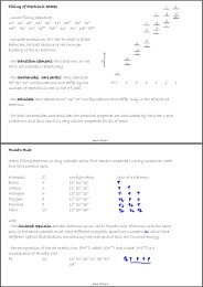
In Fig. 5, we show the potential in the θ representation as well as 

the first few energy levels for E J /E C = 1 and N g = 0. As shown in Appendix 

2, the Cooper pair box eigenenergies and eigenfunctions can be calculated 

with special functions known with arbitrary precision, and in Fig. 6 

we plot the first few eigenenergies as a function of N g for E J /E C = 0.1 

and E J /E C = 1. Thus, the Cooper box is to quantum circuit physics what 

the hydrogen atom is to atomic physics. We can modify the spectrum with 

the action of two externally controllable electrodynamic parameters: N g , 

which is directly proportional to U, and E J , which can be varied by applying 

a field through the junction or by using a split junction and applying 

a flux through the loop, as discussed in Sec. 3. These parameters bear 

some resemblance to the Stark and Zeeman fields in atomic physics. For 

the box, however much smaller values of the fields are required to change 

the spectrum entirely. 

We now limit ourselves to the two lowest levels of the box. Near the 

degeneracy point N g =1/2 where the electrostatic energy of the two charge 

states |N = 0〉 and |N = 1〉 are equal, we get the reduced hamiltonian (19,21) 

H qubit =−E z (σ Z + X control σ X ), (8) 

where, in the limit E J /E C ≪1, E z =E J /2 and X control =2(E C /E J ) ( (1/2)−N g 

) 

. 

In Eq. (8), σ Z and σ X refer to the Pauli spin operators. Note that the 

X-direction is chosen along the charge operator, the variable of the box 

we can naturally couple to. 

(a) (b) (c) 

Φ ext 

U g 

C g 

I b 

Fig. 4. The three basic superconducting qubits. (a) Cooper pair box (prototypal charge 

qubit); (b) RF-SQUID (prototypal flux qubit); and (c) current-biased junction (prototypal 

phase qubit). The charge qubit and the flux qubit requires small junctions fabricated with 

e-beam lithography while the phase qubit can be fabricated with conventional optical lithography. 

L


4 

3 

E/E J 

2 

1 

0 

-1 

-π 0 

θ 

π 

Fig. 5. Potential landscape for the phase in a Cooper pair box (thick solid line). The first 

few levels for E J /E C = 1 and N g = 1/2 are indicated by thin horizontal solid lines. 

If we plot the energy of the eigenstates of hamiltonian (8) as a 

function of the control parameter X control , we obtain the universal level 

repulsion diagram shown in Fig. 7. Note that the minimum energy 

E 

7 

6 

5 

4 

3 

2 

1 

7 

6 

E 

5 

(2E J E C ) 1/2 4 

3 

2 

1 

E J 

E C 

= 0.1 

E J 

= 1 

E C 

(2E J E C ) 1/2 N g = C g U/2e 

0 

0.5 1 1.5 2 2.5 3 

Fig. 6. Energy levels of the Cooper pair box as a function of N g , for two values of E J /E C . 

As E J /E C increases, the sensitivity of the box to variations of offset charge diminishes, but 

so does the non-linearity. However, the non-linearity is the slowest function of E J /E C and a 

compromise advantageous for coherence can be found.


1.0 

0.5 

E/E z 

0.0 

-0.5 

-1.0 

-1.0 -0.5 0.0 0.5 1.0 

X control 

Fig. 7. Universal level anticrossing found both for the Cooper pair box and the 

RF-SQUID at their “sweet spot”. 

splitting is given by E J . Comparing Eq. (8) with the spin hamiltonian 

in NMR, we see that E J plays the role of the Zeeman field while the 

electrostatic energy plays the role of the transverse field. Indeed we can 

send on the control port corresponding to U time-varying voltage signals 

in the form of NMR-type pulses and prepare arbitrary superpositions of 

states. (22) 

The expression 8 shows that at the “sweet spot” X control = 0, i.e., the 

degeneracy point N g = 1/2, the qubit transition frequency is to first order 

insentive to the offset charge noise Q r . We will discuss in Sec. 6.2 how 

an extension of the Cooper pair box circuit can display quantum coherence 

properties on long time scales by using this property. 

In general, circuits derived from the Cooper pair box have been nicknamed 

“charge qubits”. One should not think, however, that in charge 

qubits, quantum information is encoded with charge. Both the charge N 

and phase θ are quantum variables and they are both uncertain for a 

generic quantum state. Charge in “charge qubits” should be understood 

as refering to the “controlled variable”, i.e., the qubit variable that couples 

to the control line we use to write or manipulate quantum information. In 

the following, for better comparison between the three qubits, we will be 

faithful to the convention used in Eq. (8), namely that σ X represents the 

controlled variable. 

6.2. The RF-SQUID 

The second circuit—the so-called RF-SQUID (23) —can be considered 

in several ways the dual of the Cooper pair box (see Fig. 4b). It employs


3 

2 

E/E J 

1 

Φ/Φ 0 

0 

-1 -0.5 0 0.5 1 

Fig. 8. 

Schematic potential energy landcape for the RF-SQUID. 

a superconducting transformer rather than a gate capacitor to adjust the 

hamiltonian. The two sides of the junction with capacitance C J are connected 

by a superconducting loop with inductance L. An external flux 

ext is imposed through the loop by an auxiliary coil. Using the methods 

of Appendix 1, we obtain the hamiltonian (8) 

[ ] 

H = q2 

+ φ2 2e 

2C J 2L − E J cos 

(φ − ext) . (9) 

We are taking here as degrees of freedom the integral φ of the voltage 

across the inductance L, i.e., the flux through the superconducting loop, 

and its conjugate variable, the charge q on the capacitance C J ; they obey 

[φ,q] = i. Note that in this representation, the phase θ, corresponding to 

the branch flux across the Josephson element, has been eliminated. Note 

also that the flux φ, in contrast to the phase θ, takes its values on a line 

and not on a circle. Likewise, its conjugate variable q, the charge on the 

capacitance, has continuous eigenvalues and not integer ones like N. Note 

that we now have three adjustable energy scales: E J , E CJ = (2e) 2 /2C J and 

E L = 2 0 /2L. 

The potential in the flux representation is schematically shown in 

Fig. 8 together with the first few levels, which have been seen experimentally 

for the first time by the SUNY group. (24) Here, no analytical 

expressions exist for the eigenvalues and the eigenfunctions of the problem, 

which has two aspect ratios: E J /E CJ and λ = L J /L − 1. 

Whereas in the Cooper box the potential is cosine-shaped and has 

only one well since the variable θ is 2π-periodic, we have now in general 

a parabolic potential with a cosine corrugation. The idea here for curing 

the detrimental effect of the offset charge fluctuations is very different


than in the box. First of all Q stat 

r has been neutralized by shunting the two 

metallic electrodes of the junction by the superconducting wire of the loop. 

Then, the ratio E J /E CJ is chosen to be much larger than unity. This tends 

to increase the relative strength of quantum fluctuations of q, making offset 

charge fluctuations Q r small in comparison. The resulting loss in the 

non-linearity of the first levels is compensated by taking λ close to zero 

and by flux-biasing the device at the half-flux quantum value ext = 0 /2. 

Under these conditions, the potential has two degenerate wells separated 

by a shallow barrier with height E B = (3λ 2 /2)E J . This corresponds to the 

degeneracy value N g = 1/2 in the Cooper box, with the inductance energy 

in place of the capacitance energy. At ext = 0 /2, the two lowest energy 

levels are then the symmetric and antisymmetric combinations of the two 

wavefunctions localized in each well, and the energy splitting between the 

two states can be seen as the tunnel splitting associated with the quantum 

motion through the potential barrier between the two wells, bearing close 

resemblance to the dynamics of the ammonia molecule. This splitting E S 

depends exponentially on the barrier height, which itself depends strongly 

on E J .WehaveE S = η √ E B E CJ exp ( −ξ √ ) 

E B /E CJ where the numbers η 

and ξ have to be determined numerically in most practical cases. The nonlinearity 

of the first levels results thus from a subtle cancellation between 

two inductances: the superconducting loop inductance L and the junction 

effective inductance −L J0 which is opposed to L near ext = 0 /2. However, 

as we move away from the degeneracy point ext = 0 /2, the splitting 

2E between the first two energy levels varies linearly with the applied 

flux E = ζ( 2 0 /2L) (N − 1/2). Here the parameter N = ext / 0 , also 

called the flux frustration, plays the role of the reduced gate charge N g . 

The coefficient ζ has also to be determined numerically. We are therefore 

again, in the vicinity of the flux degeneracy point ext = 0 /2 and 

for E J /E CJ ≫ 1, in presence of the universal level repulsion behavior (see 

Fig. 7) and the qubit hamiltonian is again given by 

H qubit =−E z (σ Z + X control σ X ) , (10) 

where now E z = E S /2 and X control = 2(E /E S )((1/2) − N ). The qubits 

derived from this basic circuit (25,33) have been nicknamed “flux qubits”. 

Again, quantum information is not directly represented here by the flux 

φ, which is as uncertain for a general qubit state as the charge q on the 

capacitor plates of the junction. The flux φ is the system variable to which 

we couple when we write or control information in the qubit, which is 

done by sending current pulses on the primary of the RF-SQUID transformer, 

thereby modulating N , which itself determines the strength of 

the pseudo-field in the X-direction in the hamiltonian 10. Note that the


parameters E S , E , and N are all influenced to some degree by the critical 

current noise, the dielectric noise and the charge noise. Another independent 

noise can also be present, the noise of the flux in the loop, which 

is not found in the box and which will affect only N . Experiments on 

DC-SQUIDS (15) have shown that this noise, in adequate conditions, can 

be as low as 10 −8 (h/2e)/Hz −1/2 at a few kHz. However, experimental 

results on flux qubits (see below) seem to indicate that larger apparent flux 

fluctuations are present, either as a result of flux trapping or critical current 

fluctuations in junctions implementing inductances. 

6.3. Current-biased Junction 

The third basic quantum circuit biases the junction with a fixed 

DC-current source (Fig. 7c). Like the flux qubit, this circuit is also 

insensitive to the effect of offset charge and reduces the effect of charge 

fluctuations by using large ratios of E J /E CJ . A large non-linearity in the 

Josephson inductance is obtained by biasing the junction at a current I 

very close to the critical current. A current bias source can be understood 

as arising from a loop inductance with L →∞ biased by a flux →∞ 

such that I = /L. The Hamiltonian is given by 

H = E CJ p 2 − Iϕ 0 δ − I 0 ϕ 0 cos δ, (11) 

where the gauge invariant phase difference operator δ is, apart from the 

scale factor ϕ 0 , precisely the branch flux across C J . Its conjugate variable 

is the charge 2ep on that capacitance, a continuous operator. We 

have thus [δ,p] = i. The variable δ, like the variable φ of the RF-SQUID, 

takes its value on the whole real axis and its relation with the phase θ is 

δ mod 2π = θ as in our classical analysis of Sec. 4. 

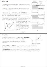
The potential in the δ representation is shown in Fig. 9. It has the 

shape of a tilted washboard, with the tilt given by the ratio I/I 0 . When 

I approaches I 0 , the phase is δ ≈ π/2, and in its vicinity, the potential is 

very well approximated by the cubic form 

U (δ) = ϕ 0 (I 0 − I)(δ − π/2) − I 0ϕ 0 

6 (δ − π/2)3 , (12) 

Note that its shape depends critically on the difference I 0 − I. ForI I 0 , 

there is a well with a barrier height U = (2 √ 2/3)I 0 ϕ 0 (1 − I/I 0 ) 3/2 and 

the classical oscillation frequency at the bottom of the well (so-called 

plasma oscillation) is given by


2 

E/E J 

0 

-2 

-4 

-1 -0.5 0 0.5 1 

δ/2π 

Fig. 9. 

Tilted washboard potential of the current-biased Josephson junction. 

ω p = 

= 

1 

√ 

LJ (I)C J 

1 

√ 

[1 − (I/I 0 ) 2] 1/4 

. 

LJ0 C J 

Quantum-mechanically, energy levels are found in the well (see Fig. 11) (3) 

with non-degenerate spacings. The first two levels can be used for qubit 

states, (26) and have a transition frequency ω 01 ≃ 0.95ω p . 

A feature of this qubit circuit is built-in readout, a property missing 

from the two previous cases. It is based on the possibility that states in 

the cubic potential can tunnel through the cubic potential barrier into the 

continuum outside the barrier. Because the tunneling rate increases by 

a factor of approximately 500 each time we go from one energy level to 

the next, the population of the |1〉 qubit state can be reliably measured by 

sending a probe signal inducing a transition from the 1 state to a higher 

energy state with large tunneling probability. After tunneling, the particle 

representing the phase accelerates down the washboard, a convenient 

self-amplification process leading to a voltage as large as 2/e across the 

junction. Therefore, a finite voltage V ≠ 0 suddenly appearing across the 

junction just after the probe signal implies that the qubit was in state |1〉, 

whereas V = 0 implies that the qubit was in state |0〉. 

In practice, like in the two previous cases, the transition frequency 

ω 01 /2π falls in the 5–20 GHz range. This frequency is only determined by 

material properties of the barrier, since the product C J L J does not depend 

on junction area. The number of levels in the well is typically U/ω p ≈4.


Setting the bias current at a value I and calling I the variations of 

the difference I − I 0 (originating either in variations of I or I 0 ), the qubit 

Hamiltonian is given by 

√ 

 

H qubit = ω 01 σ Z + I (σ X + χσ Z ), (13) 

2ω 01 C J 

where χ = √ ω 01 /3U ≃1/4 for typical operating parameters. In contrast 

with the flux and phase qubit circuits, the current-biased Josephson junction 

does not have a bias point where the 0→1 transition frequency has a 

local minimum. The hamiltonian cannot be cast into the NMR-type form 

of Eq. (8). However, a sinusoidal current signal I (t) ∼ sin ω 01 t can still 

produce σ X rotations, whereas a low-frequency signal produces σ Z operations. 

(27) 

In analogy with the preceding circuits, qubits derived from this circuit 

and/or having the same phase potential shape and qubit properties have 

been nicknamed “phase qubits” since the controlled variable is the phase 

(the X pseudo-spin direction in hamiltonian (13)). 

6.4. Tunability versus Sensitivity to Noise in Control Parameters 

The reduced two-level hamiltonians Eqs. (8), (10) and (13) have been 

tested thoroughly and are now well-established. They contain the very 

important parametric dependence of the coefficient of σ X , which can be 

viewed on one hand as how much the qubit can be tuned by an external 

control parameter, and on the other hand as how much it can be dephased 

by uncontrolled variations in that parameter. It is often important to realize 

that even if the control parameter has a very stable value at the level of 

room-temperature electronics, the noise in the electrical components relaying 

its value at the qubit level might be inducing detrimental fluctuations. 

An example is the flux through a superconducting loop, which in principle 

could be set very precisely by a stable current in a coil, and which in 

practice often fluctuates because of trapped flux motion in the wire of the 

loop or in nearby superconducting films. Note that, on the other hand, 

the two-level hamiltonian does not contain all the non-linear properties of 

the qubit, and how they conflict with its intrinsic noise, a problem which 

we discuss in the next Sec. 6.5. 

6.5. Non-linearity versus Sensitivity to Intrinsic Noise 

The three basic quantum circuit types discussed above illustrate a general 

tendency of Josephson qubits. If we try to make the level structure


very non-linear, i.e. |ω 01 − ω 12 | ≫ ω 01 , we necessarily expose the system 

sensitively to at least one type of intrinsic noise. The flux qubit is contructed 

to reach a very large non-linearity, but is also maximally exposed, relatively 

speaking, to critical current noise and flux noise. On the other hand, 

the phase qubit starts with a relatively small non-linearity and acquires it 

at the expense of a precise tuning of the difference between the bias current 

and the critical current, and therefore exposes itself also to the noise 

in the latter. The Cooper box, finally, acquires non-linearity at the expense 

of its sensitivity to offset charge noise. The search for the optimal qubit 

circuit involves therefore a detailed knowledge of the relative intensities of 

the various sources of noise, and their variations with all the construction 

parameters of the qubit, and in particular—this point is crucial—the properties 

of the materials involved in the tunnel junction fabrication. Such indepth 

knowledge does not yet exist at the time of this writing and one can 

only make educated guesses. 

The qubit optimization problem is also further complicated by the 

necessity to readout quantum information, which we address just after 

reviewing the relationships between the intensity of noise and the decay 

rates of quantum information. 

7. QUBIT RELAXATION AND DECOHERENCE 

A generic quantum state of a qubit can be represented as a unit vector 

−→ S pointing on a sphere—the so-called Bloch sphere. One distinguishes 

two broad classes of errors. The first one corresponds to the tip of the 

Bloch vector diffusing in the latitude direction, i.e., along the arc joining 

the two poles of the sphere to or away from the north pole. This process is 

called energy relaxation or state-mixing. The second class corresponds to 

the tip of the Bloch vector diffusing in the longitude direction, i.e., perpendicularly 

to the line joining the two poles. This process is called dephasing 

or decoherence. 

In Appendix 3, we define precisely the relaxation and decoherence 

rates and show that they are directly proportional to the power spectral 

densities of the noises entering in the parameters of the hamiltonian of 

the qubit. More precisely, we find that the decoherence rate is proportional 

to the total spectral density of the quasi-zero-frequency noise in the qubit 

Larmor frequency. The relaxation rate, on the other hand, is proportional 

to the total spectral density, at the qubit Larmor frequency, of the noise 

in the field perpendicular to the eigenaxis of the qubit. 

In principle, the expressions for the relaxation and decoherence rate 

could lead to a ranking of the various qubit circuits: from their reduced


spin hamiltonian, one can find with what coefficient each basic noise 

source contributes to the various spectral densities entering in the rates. 

In the same manner, one could optimize the various qubit parameters to 

make them insensitive to noise, as much as possible. However, before discussing 

this question further, we must realize that the readout itself can 

provide substantial additional noise sources for the qubit. Therefore, the 

design of a qubit circuit that maximizes the number of coherent gate operations 

is a subtle optimization problem which must treat in parallel both 

the intrinsic noises of the qubit and the back-action noise of the readout. 

8. READOUT OF SUPERCONDUCTING QUBITS 

8.1. Formulation of the Readout Problem 

We have examined so far the various basic circuits for qubit implementation 

and their associated methods to write and manipulate quantum 

information. Another important task quantum circuits must perform is the 

readout of that information. As we mentioned earlier, the difficulty of the 

readout problem is to open a coupling channel to the qubit for extracting 

information without at the same time submitting it to both dissipation and 

noise. 

Ideally, the readout part of the circuit—referred to in the following 

simply as “readout”—should include both a switch, which defines an 

“OFF” and an “ON” phase, and a state measurement device. During the 

OFF phase, where reset and gate operations take place, the measurement 

device should be completely decoupled from the qubit degrees of freedom. 

During the ON phase, the measurement device should be maximally coupled 

to a qubit variable that distinguishes the 0 and the 1 state. However, 

this condition is not sufficient. The back-action of the measurement device 

during the ON phase should be weak enough not to relax the qubit. (28) 

The readout can be characterized by 4 parameters. The first one 

describes the sensitivity of the measuring device while the next two 

describe its back-action, factoring in the quality of the switch (see Appendix 

3 for the definitions of the rates Ɣ): 

(i) the measurement time τ m defined as the time taken by the measuring 

device to reach a signal-to-noise ratio of 1 in the determination of the 

state. 

(ii) the energy relaxation rate Ɣ1 ON of the qubit in the ON state. 

(iii) the coherence decay rate Ɣ2 OFF of the qubit information in the OFF 

state.


(iv) the dead time t d needed to reset both the measuring device and qubit 

after a measurement. They are usually perturbed by the energy expenditure 

associated with producing a signal strong enough for external 

detection. 

Simultaneously minimizing these parameters to improve readout performance 

cannot be done without running into conflicts. An important 

quantity to optimize is the readout fidelity. By construction, at the end of 

the ON phase, the readout should have reached one of two classical states: 

0 c and 1 c , the outcomes of the measurement process. The latter can be 

described by two probabilities: the probability p 00c (p 11c ) that starting from 

the qubit state |0〉 (|1〉) the measurement yields 0 c (1 c ). The readout fidelity 

(or discriminating power) is defined as F = p 00c + p 11c − 1. For a measuring 

device with a signal-to-noise ratio increasing like the square of measurement 

duration τ, we would have, if back-action could be neglected, 

F = erf ( 2 −1/2 τ/τ m 

) 

. 

8.2. Requirements and General Strategies 

The fidelity and speed of the readout, usually not discussed in the 

context of quantum algorithms because they enter marginally in the evaluation 

of their complexity, are actually key to experiments studying the 

coherence properties of qubits and gates. A very fast and sensitive readout 

will gather at a rapid pace information on the imperfections and drifts 

of qubit parameters, thereby allowing the experimenter to design fabrication 

strategies to fight them during the construction or even correct them 

in real time. 

We are thus mostly interested in “single-shot” readouts, (28) for which 

F is of order unity, as opposed to schemes in which a weak measurement 

is performed continuously. (29) If F ≪1, of order F −2 identical preparation 

and readout cycles need to be performed to access the state of the qubit. 

The condition for “single-shot” operation is 

Ɣ ON 

1 

τ m < 1. 

The speed of the readout, determined both by τ m and t d , should be 

sufficiently fast to allow a complete characterization of all the properties 

of the qubit before any drift in parameters occurs. With sufficient speed, 

the automatic correction of these drits in real time using feedback will be 

possible. 

Rapidly pulsing the readout to full ON and OFF states is done with 

a fast, strongly non-linear element, which is provided by one or more


auxiliary Josephson junctions. Decoupling the qubit from the readout in 

the OFF phase requires balancing the circuit in the manner of a Wheatstone 

bridge, with the readout input variable and the qubit variable corresponding 

to two orthogonal electrical degrees of freedom. Finally, to be as 

complete as possible even in presence of small asymmetries, the decoupling 

also requires an impedance mismatch between the qubit and the dissipative 

degrees of freedom of the readout. In Sec. 8.3, we discuss how these 

general ideas have been implemented in second generation quantum circuits. 

The examples we have chosen all involve a readout circuit which is 

built-in the qubit itself to provide maximal coupling during the ON phase, 

as well as a decoupling scheme which has proven effective for obtaining 

long decoherence times. 

8.3. Phase Qubit: Tunneling Readout with a DC-SQUID On-chip 

Amplifier. 

The simplest example of a readout is provided by a system derived 

from the phase qubit (see Fig. 10). In the phase qubit, the levels in the 

cubic potential are metastable and decay in the continuum, with level n+1 

having roughly a decay rate Ɣ n+1 that is 500 times faster than the decay 

Ɣ n of level n. This strong level number dependence of the decay rate leads 

naturally to the following readout scheme: when readout needs to be performed, 

a microwave pulse at the transition frequency ω 12 (or better at 

ω 13 ) transfers the eventual population of level 1 into level 2, the latter 

decaying rapidly into the continuum, where it subsequently loses energy 

by friction and falls into the bottom state of the next corrugation of the 

potential (because the qubit junction is actually in a superconducting loop 

of large but finite inductance, the bottom of this next corrugation is in fact 

the absolute minimum of the potential and the particle representing the 

system can stay an infinitely long time there). Thus, at the end of the readout 

pulse, the sytem has either decayed out of the cubic well (readout state 

1 c ) if the qubit was in the |1〉 state or remained in the cubic well (readout 

state 0 c ) if the qubit was in the |0〉 state. The DC-SQUID amplifier 

is sensitive enough to detect the change in flux accompanying the exit of 

the cubic well, but the problem is to avoid sending the back-action noise 

of its stabilizing resistor into the qubit circuit. The solution to this problem 

involves balancing the SQUID loop in such a way, that for readout 

state 0 c , the small signal gain of the SQUID is zero, whereas for readout 

state 1 c , the small signal gain is non-zero. (17) This signal dependent gain is 

obtained by having two junctions in one arm of the SQUID whose total 

Josephson inductance equals that of the unique junction in the other arm.


WRITE AND 

CONTROL 

PORT 

READOUT 

PORT 

Fig. 10. Phase qubit implemented with a Josephson junction in a high-inductance superconducting 

loop biased with a flux sufficiently large that the phase across the junction sees 

a potential analogous to that found for the current-biased junction. The readout part of the 

circuit is an asymmetric hysteretic SQUID which is completely decoupled from the qubit in 

the OFF phase. Isolation of the qubit both from the readout and control port is obtained 

through impedance mismatch of transformers. 

Fig. 11. Rabi oscillations observed for the qubit of Fig. 10. 

Finally, a large impedance mismatch between the SQUID and the qubit is 

obtained by a transformer. The fidelity of such readout is remarkable: 95% 

has been demonstrated. In Fig. 11, we show the result of a measurement 

of Rabi oscillations with such qubit+readout.


WRITE AND 

CONTROL PORT 

READOUT 

PORT 

Fig. 12. “Quantronium" circuit consisting of a Cooper-pair box with a non-linear inductive 

readout. A Wheatstone bridge configuration decouples qubit and readout variables when 

readout is OFF. Impedance mismatch isolation is also provided by additional capacitance in 

parallel with readout junction. 

8.4. Cooper-pair Box with Non-linear Inductive Readout: The 

“Quantronium” Circuit 

The Cooper-pair box needs to be operated at its “sweet spot” (degeneracy 

point) where the transition frequency is to first order insensitive to 

offset charge fluctuations. The “Quantronium” circuit presented in Fig. 12 

is a 3-junction bridge configuration with two small junctions defining a 

Cooper box island, and thus a charge-like qubit which is coupled capacitively 

to the write and control port (high-impedance port). There is also 

a large third junction, which provides a non-linear inductive coupling to 

the read port. When the read port current I is zero, and the flux through 

the qubit loop is zero, noise coming from the read port is decoupled 

from the qubit, provided that the two small junctions are identical both in 

critical current and capacitance. When I is non-zero, the junction bridge is 

out of balance and the state of the qubit influences the effective non-linear 

inductance seen from the read port. A further protection of the impedance 

mismatch type is obtained by a shunt capacitor across the large junction: 

at the resonance frequency of the non-linear resonator formed by 

the large junction and the external capacitance C, the differential mode 

of the circuit involved in the readout presents an impedance of the order 

of an ohm, a substantial decoupling from the 50 transmission line carrying 

information to the amplifier stage. The readout protocol involves a 

DC pulse (22,30) or an RF pulse (31) stimulation of the readout mode. The 

response is bimodal, each mode corresponding to a state of the qubit. 

Although the theoretical fidelity of the DC readout can attain 95%, only a 

maximum of 40% has been obtained so far. The cause of this discrepancy 

is still under investigation. 

In Fig. 13 we show the result of a Ramsey fringe experiment demonstrating 

that the coherence quality factor of the quantronium can reach


Fig. 13. Measurement of Ramsey fringes for the Quantronium. Two π/2 pulses separated 

by a variable delay are applied to the qubit before measurement. The frequency of the pulse 

is slightly detuned from the transition frequency to provide a stroboscopic measurement of 

the Larmor precession of the qubit. 

25,000 at the sweet spot. (22) By studying the degradation of the qubit 

absorption line and of the Ramsey fringes as one moves away from the 

sweet spot, it has been possible to show that the residual decoherence is 

limited by offset charge noise and by flux noise. (32) In principle, the influence 

of these noises could be further reduced by a better optimization 

of the qubit design and parameters. In particular, the operation of the 

box can tolerate ratios of E J /E C around 4 where the sensitivity to offset 

charge is exponentially reduced and where the non-linearity is still of order 

15%. The quantronium circuit has so far the best coherence quality factor. 

We believe this is due to the fact that critical current noise, one dominant 

intrinsic source of noise, affects this qubit far less than the others, relatively 

speaking, as can be deduced from the qubit hamiltonians of Sec. 6. 

8.5. 3-Junction Flux Qubit with Built-in Readout 

Figure 14 shows a third example of built-in readout, this time for 

a flux-like qubit. The qubit by itself involves three junctions in a loop, 

the larger two of the junctions playing the role of the loop inductance 

in the basic RF-SQUID. (33) The advantage of this configuration is to 

reduce the sensitivity of the qubit to external flux variations. The readout 

part of the circuit involves two other junctions forming a hysteretic 

DC-SQUID whose offset flux depends on the qubit flux state. The critical 

current of this DC-SQUID has been probed by a DC pulse, but an


READOUT 

PORT 

WRITE AND 

CONTROL 

PORT 

Fig. 14. Three-junction flux qubit with a non-linear inductive readout. The medium-size 

junctions play the role of an inductor. Bridge configuration for nulling out back-action of 

readout is also employed here, as well as impedance mismatch provided by additional capacitance. 

Fig. 15. Ramsey fringes obtained for qubit of Fig. 14. 

RF pulse could be applied as in another flux readout. Similarly to the two 

previous cases, the readout states 1 c and 0 c , which here correspond to the 

DC-SQUID having switched or not, map very well the qubit states |1〉 and 

|0〉, with a fidelity better than 60%. Here also, a bridge technique orthogonalizes 

the readout mode, which is the common mode of the DC-SQUID, 

and the qubit mode, which is coupled to the loop of the DC-SQUID. 

External capacitors provide additional protection through impedance mismatch. 

Figure 15 shows Ramsey oscillations obtained with this system.


8.6. Too much On-chip Dissipation is Problematic: Do not Stir up the Dirt 

All the circuits above include an on-chip amplification scheme producing 

high-level signals which can be read directly by high-temperature 

low-noise electronics. In the second and third examples, these signals lead 

to non-equilibrium quasi-particle excitations being produced in the near 

vicinity of the qubit junctions. An elegant experiment has recently demonstrated 

that the presence of these excitations increases the offset charge 

noise. (34) More generally, one can legitimately worry that large energy 

dissipation on the chip itself will lead to an increase of the noises discussed 

in Sec. 5.2. A broad class of new readout schemes addresses this 

question. (31,35,36) They are based on a purely dispersive measurement of 

a qubit susceptibility (capacitive or inductive). A probe signal is sent 

to the qubit. The signal is coupled to a qubit variable whose average 

value is identical in the two qubit states (for instance, in the capacitive 

susceptibility, the variable is the island charge in the charge qubit at the 

degeneracy point). However, the susceptibility, which is the derivative of 

the qubit variable with respect to the probe, differs from one qubit state 

to the other. The resulting state-dependent phase shift of the reflected signal 

is thus amplified by a linear low temperature amplifier and finally discriminated 

at high temperature against an adequately chosen threshold. 

In addition to being very thrifty in terms of energy being dissipated on 

chip, these new schemes also provide a further natural decoupling action: 

when the probe signal is off, the back-action of the amplifier is also completely 

shut off. Finally, the interrogation of the qubit in a frequency band 

excluding zero facilitates the design of very efficient filters. 

9. COUPLING SUPERCONDUCTING QUBITS 

A priori, three types of coupling scheme can be envisioned: 

(a) In the first type, the transition frequency of the qubits are all equal 

and the coupling between any pair is switched on using one or several 

junctions as non-linear elements. (37,38) 

(b) In the second type, the couplings are fixed, but the transition frequencies 

of a pair of qubits, originally detuned, are brought on resonance 

when the coupling between them needs to be turned on. (39–41) 

(c) In the third type, which bears close resemblance to the methods used 

in NMR, (1) the couplings and the resonance frequencies of the qubits 

remain fixed, the qubits being always detuned. Being off-diagonal, 

the coupling elements have negligible action on the qubits. However, 

when a strong micro-wave field is applied to the target and control


qubits their resonant frequency with an appropriate amplitude, they 

become in “speaking terms” for the exchange of energy quanta and 

gate action can take place. (42) 

So far only scheme (b) has been tested experimentally. 

The advantage of schemes (b) and (c) is that they work with purely 

passive reactive elements like capacitors and inductors which should 

remain very stable as a function of time and which also should present 

very little high-frequency noise. In a way, we must design quantum integrated 

circuits in the manner that vacuum tube radios were designed in 

the 1950s: only six tubes were used for a complete heterodyne radio set, 

including the power supply. Nowadays several hundreds of transistors are 

used in a radio or any hi-fi system. In that ancient era of classical electronics, 

linear elements like capacitors, inductors or resistors were “free” 

because they were relatively reliable whereas tubes could break down easily. 

We have to follow a similar path in quantum integrated circuit, the reliability 

issues having become noise minimization issues. 

10. CAN COHERENCE BE IMPROVED WITH BETTER 

MATERIALS? 

Up to now, we have discussed how, given the power spectral densities 

of the noises Q r , E C and E J , we could design a qubit equipped 

with control, readout and coupling circuits. It is worthwhile to ask at this 

point if we could improve the material properties to improve the coherence 

of the qubit, assuming all other problems like noise in the control 

channels and the back-action of the readout have been solved. A model 

put forward by one of us (JMM) and collaborators shed some light on 

the direction one would follow to answer this question. The 1/f spectrum 

of the materials noises suggests that they all originate from 2-level 

fluctuators in the amorphous alumina tunnel layer of the junction itself, 

or its close vicinity. The substrate or the surface of the superconducting 

films are also suspect in the case of Q r and E C but their influence 

would be relatively weaker and we ignore them for simplicity. These twolevel 

systems are supposed to be randomly distributed positional degrees 

of freedom ξ i with effective spin-1/2 properties, for instance an impurity 

atom tunneling between two adjacent potential well. Each two-level system 

is in principle characterized by three parameters: the energy splitting 

ω i , and the two coefficients α i and β i of the Pauli matrix representation 

of ξ i = α i σ iz + β i σ ix (z is here by definition the eigen-energy axis). 

The random nature of the problem leads us to suppose that α i and β i 

are both Gaussian random variables with the same standard deviation ρ i .


By carrying a charge, the thermal and quantum motion of ξ i can contribute 

to Q r = ∑ i q iξ i and E C = ∑ i c i β2 i 

ω i 

σ iz . Likewise, by modifying the 

transmission of a tunneling channel in its vicinity, the motion of ξ i can 

contribute to E J = ∑ i g iξ i . We can further suppose that the quality of 

the material of the junction is simply characterized by a few numbers. The 

essential one is the density ν of the transition frequencies ω i in frequency 

space and in real space, assuming a ω −1 distribution (this is necessary to 

explain the 1/f behavior) and a uniform spatial distribution on the surface 

of the junction. Recent experiments indicate that the parameter ν is 

of order 10 5 µm −2 per decade. Then, assuming a value for ρ i independent 

of frequency, only one coefficient is needed per noise, namely, the average 

modulation efficiency of each fluctuator. Such analysis provides a common 

language for describing various experiments probing the dependence of decoherence 

on the material of the junction. Once the influence of the junction 

fabrication parameters (oxydation pressure and temperature, impurity 

contents, and so on) on these noise intensities will be known, it will be 

possible to devise optimized fabrication procedures, in the same way perhaps 

as the 1/f noise in C-MOS transistors has been reduced by careful 

material studies. 

11. CONCLUDING REMARKS AND PERSPECTIVES 

The logical thread through this review of superconducting qubits has 

been the question “What is the best qubit design?”. Because some crucial 

experimental data is still missing, we unfortunately, at present, cannot conclude 

by giving a definitive answer to this complex optimization problem. 

Yet, a lot has already been achieved, and superconducting qubits are 

becoming serious competitors of trapped ions and atoms. The following 

properties of quantum circuits have been demonstrated: 

(a) Coherence quality factors Q ϕ = T ϕ ω 01 can attain at least 2×10 4 . 

(b) Readout and reset fidelity can be greater than 95%. 

(c) All states on the Bloch sphere can be addressed. 

(d) Spin echo techniques can null out low frequency drift of offset 

charges. 

(e) Two qubits can be coupled and RF pulses can implement gate operation. 

(f) A qubit can be fabricated using only optical lithography techniques. 

The major problem we are facing is that these various results have not 

been obtained at the same time IN THE SAME CIRCUIT, although succesful 

design elements in one have often been incorporated into the next


generation of others. The complete optimization of the single qubit+readout 

has not been achieved yet. However, we have presented in this review 

the elements of a systematic methodology resolving the various conflicts 

that are generated by all the different requirements. Our opinion is that, 

once noise sources are better characterized, an appropriate combination 

of all the known circuit design strategies for improving coherence, as well 

as the understanding of optimal tunnel layer growth conditions for lowering 

the intrinsic noise of Josephson junctions, should lead us to reach 

the 1-qubit and 2-qubit coherence levels needed for error correction. (45) 

Along the way, good medium term targets to test overall progress on 

the simultaneous fronts of qubit coherence, readout and gate coupling 

are the measurement of Bell ’s inequality violation or the implementation 

of the Deutsch–Josza algorithm, both of which requiring the simultaneous 

satisfaction of properties (a)–(e). 

ACKNOWLEDGMENTS 

The authors have greatly benefited from discussions with I. Chuang, 

D. Esteve, S. Girvin, S. Lloyd, H. Mooij, R. Schoelkopf, I. Siddiqi, C. Urbina 

and D. Vion. They would like also to thank the participants of the 

Les Houches Summer School on Quantum Information Processing and 

Entanglement held in 2003 for useful exchanges. Finally, funding from 

ARDA/ARO and the Keck Fundation is gratefully acknowledged. 

APPENDIX 1. QUANTUM CIRCUIT THEORY 

The problem we are addressing in this section is, given a superconducting 

circuit made up of capacitors, inductors and Josephson junctions, 

how to systematically write its quantum hamiltonian, the generating function 

from which the quantum dynamics of the circuit can be obtained. 

This problem has been considered first by Yurke and Denker (46) in a seminal 

paper and analyzed in further details by Devoret. (47) We will only 

summarize here the results needed for this review. 

The circuit is given as a set of branches, which can be capacitors, 

inductors or Josephson tunnel elements, connected at nodes. Several independent 

paths formed by a succession of branches can be found between 

nodes. The circuit can therefore contain one or several loops. It is important 

to note that a circuit has not one hamiltonian but many, each one 

depending on a particular representation. We are describing here one


particular type of representation, which is usually well adapted to circuits 

containing Josephson junctions. Like in classical circuit theory, a 

set of independent current and voltages has to be found for a particular 

representation. We start by associating to each branch b of the circuit, the 

current i b flowing through it and the voltage v b across it (a convention has 

to be made first on the direction of the branches). Kirchhoff’s laws impose 

relations among branch variables and some of them are redundant. The 

following procedure is used to eliminate redundant branches: one node of 

the circuit is first chosen as ground. Then from the ground, a loop-free 

set of branches called spanning tree is selected. The rule behind the selection 

of the spanning tree is the following: each node of the circuit must be 

linked to the ground by one and only one path belonging to the tree. In 

general, inductors (linear or non-linear) are preferred as branches of the 

tree but this is not necessary. Once the spanning tree is chosen (note that 

we still have many possibilities for this tree), we can associate to each node 

a “node voltage” v n which is the algebraic sum of the voltages along the 

branches between ground and the node. The conjugate “node current” i n 

is the algebraic sum of all currents flowing to the node through capacitors 

ONLY. The dynamical variables appearing in the hamiltonian of the 

circuit are the node fluxes and node charges defined as 

φ n = 

q n = 

∫ t 

−∞ 

∫ t 

−∞ 

v (t 1 ) dt 1 , 

i (t 1 ) dt 1 . 

Using Kirchhoff’s laws, it is possible to express the flux and the 

charge of each branch as a linear combination of all the node fluxes 

and charges, respectively. In this inversion procedure, important physical 

parameters appear: the magnetic fluxes through the loops imposed by 

external static magnetic fields and the polarization charges imposed by 

charge bias sources. 

If we now sum the energies of all branches of the circuit expressed 

in terms of node flux and charges, we will obtain the hamiltonian of 

the circuit corresponding to the representation associated with the particular 

spanning tree. In this hamiltonian, capacitor energies behave like 

kinetic terms while the inductor energies behave as potential terms. The 

hamiltonian of the LC circuit written in Sec. 2 is an elementary example 

of this procedure. 

Once the hamiltonian is obtained it is easy get its quantum version by 

replacing all the node fluxes and charges by their quantum operator equivalent. 

The flux and charge of a node have a commutator given by i, like


the position and momentum of a particle 

φ → ˆφ, 

q →ˆq, 

[ 

ˆφ, ˆq] 

= i. 

One can also show that the flux and charge operators corresponding 

to a branch share the same commutation relation. Note that for the special 

case of the Josephson element, the phase ˆθ and Cooper pair number 

ˆN, which are its dimensionless electric variables, have the property 

[ 

ˆθ, ˆN] 

= i. 

In the so-called charge basis, we have 

ˆN = ∑ N 

N |N〉〈N| , 

cos ˆθ = 

2 

1 ∑ 

(|N〉〈N + 1| + |N+〉〈N|) 

N 

while in the so-called phase basis, we have 

ˆN = |θ〉 ∂ 

i∂ 〈θ| . 

Note that since the Cooper pair number ˆN is an operator with integer 

eigenvalues, its conjugate variable ˆθ, has eigenvalues behaving like angles, 

i.e., they are defined only modulo 2π. 

In this review, outside this appendix, we have dropped the hat on 

operators for simplicity. 

APPENDIX 2. EIGENENERGIES AND EIGENFUNCTIONS 

OF THE COOPER PAIR BOX 

From Appendix 1, it easy to see that the hamiltonian of the Cooper 

pair box leads to the Schrodinger equation 

[ ( ) ∂ 2 

E C 

i∂θ − N g − E J cos θ] 

k (θ) = E k k (θ).


The functions k (θ) e −iN g 

and energies E k are solutions of the Mathieu 

equation and can be found with arbitrary precision for all values of 

the parameters N g and E J /E C . (48) For instance, using the program Mathematica, 

we find 

[ 

] 

E k = E C M A k + 1 − (k + 1) mod 2 + 2N g (−1) k , −2E J /E C , 

{ [ 

k (θ) = eiN gθ 4Ek 

√ M C , −2E J 

, θ ] 

[ 

+ i(−1) k+1 4Ek 

M S , −2E J 

, θ ]} 

, 

2π E C E C 2 

E C E C 2 

where M A (r, q) = MathieuCharacteristicA[r,q], 

M C (a,q,z) = MathieuC[a,q,z], 

M S (a,q,z) = MathieuS[a,q,z]. 

APPENDIX 3. RELAXATION AND DECOHERENCE RATES 

FOR A QUBIT 

Definition of the Rates 

We start by introducing the spin eigenreference frame ẑ, ˆx and ŷ consisting 

of the unit vector along the eigenaxis and the associated orthogonal 

unit vectors ( ˆx is in the XZ plane). For instance, for ( the Cooper pair box, 

we find that ẑ = cos αẐ + sin α ˆX, with tan α = 2E C Ng − 1/2 ) /E J , while 

ˆx =−sin αẐ + cos α ˆX. 

Starting with −→ S pointing along ˆx at time t = 0, the dynamics of the 

Bloch vector in absence of relaxation or decoherence is 

−→ S 0 (t) = cos(ω 01 ) ˆx + sin(ω 01 )ŷ 

In presence of relaxation and decoherence, the Bloch vector will deviate 

from −→ S 0 (t) and will reach eventually the equilibrium value Sz eq ẑ, 

where Sz 

eq = tanh (ω 01 /2k B T). 

We define the relaxation and decoherence rates as 

ln 〈 S z (t) − S eq 〉 

z 

Ɣ 1 = lim 

, 

t→∞ t ] 

ln 

Ɣ φ = lim t→∞ 

[ 〈 −→S (t). 

−→ S 0 (t)〉 

∣ −→ S(t)−Sz 

eq 

ẑ∣ 

Note that these rates have both a useful and rigorous meaning only if 

the evolution of the components of the average Bloch vector follows, after 

t 

.


a negligibly short settling time, an exponential decay. The Ɣ 1 and Ɣ φ rates 

are related to the NMR spin relaxation times T 1 and T 2 (49) by 

T 1 = Ɣ −1 

1 , 

T 2 = ( Ɣ φ + Ɣ 1 /2 ) −1 . 

The T 2 time can be seen as the net decay time of quantum information, 

including the influence of both relaxation and dephasing processes. 

In our discussion of superconducting qubits, we must separate the contribution 

of the two type of processes since their physical origin is in general 

very different and cannot rely on the T 2 time alone. 

Expressions for the Rates 

The relaxation process can be seen as resulting from unwanted transitions 

between the two eigenstate of the qubit induced by fluctuations in 

the effective fields along the x and y axes. Introducing the power spectral 

density of this field, one can demonstrate from Fermi’s Golden Rule that, 

for perturbative fluctuations, 

Ɣ 1 = S x(ω 01 ) + S y (ω 01 ) 

2 . 

Taking the case of the Cooper-pair box as an example, we find that 

S y (ω 01 ) = 0 and that 

where 

S x (ω) = 

∫ +∞ 

−∞ 

dt e iωt 〈A(t)A(0)〉 + 〈B(t)B(0)〉 , 

A(t) = E J(t)E el 

√ , 

2 EJ 2 + E2 el 

B(t) = E JE el (t) 

√ , 

2 EJ 2 + E2 el 

E el = 2E C (N g − 1/2). 

Since the fluctuations E el (t) can be related to the impedance of the 

environment of the box, (19,21,50) an order of magnitude estimate of the 

relaxation rate can be performed, and is in rough agreement with observations. 

(22,51)


The decoherence process, on the other hand, is induced by fluctuations 

in the effective field along the eigenaxis z. If these fluctuations are 

Gaussian, with a white noise spectral density up to frequencies of order 

several Ɣ φ (which is often not the case because of the presence of 1/f 

noise) we have 

Ɣ φ = S z (ω ≃ 0) 

2 . 

In presence of a low frequency noise with an 1/f behavior, the formula 

is more complicated. (52) If the environment producing the low frequency 

noise consists of many degrees of freedom, each of which is very weakly 

coupled to the qubit, then one is in presence of classical dephasing which, 

if slow enough, can in principle be fought using echo techniques. If, one 

the other hand, only a few degrees of freedom like magnetic spins or 

glassy two-level systems are dominating the low frequency dynamics, dephasing 

is quantum and not correctable, unless the transition frequencies of 

these few perturbing degrees of freedom is itself very stable. 

REFERENCES 

1. M. A. Nielsen and I. L. Chuang, Quantum Computation and Quantum Information (Cambridge, 

2000). 

2. M. Tinkham, Introduction to Superconductivity (Krieger, Malabar, 1985). 

3. J. M. Martinis, M. H. Devoret, J. Clarke, Phys. Rev. Lett. 55, 1543 (1985); M. H. Devoret, 

J. M. Martinis, J. Clarke, Phys. Rev. Lett. 55, 1908 (1985); J. M. Martinis, M. H. 

Devoret and J. Clarke, Phys. Rev. 35, 4682 (1987). 

4. J. M. Martinis and M. Nahum, Phys Rev. B48, 18316 (1993). 

5. B. D. Josephson, in Superconductivity, R. D. Parks (ed.) (Marcel Dekker, New York, 

1969). 

6. K. K. Likharev, Dynamics of Josephson Junctions and Circuits (Gordon and Breach, New 

York, 1986). 

7. I. Giaever, Phys. Rev. Lett. 5, 147, 464 (1960). 

8. A. O. Caldeira and A. J. Leggett, Ann. Phys. (N.Y.) 149, 347 (1983); A. J. Leggett, 

J. Phys. CM 14, R415 (2002). 

9. D. P. DiVincenzo, arXiv:quant-ph/0002077. 

10. R. P. Feynman, Lectures on Physics, Vol. 2, Chap. 23, (Addison-Wesley, Reading, 1964). 

11. D. C. Mattis and J. Bardeen, Phys. Rev. 111, 412 (1958). 

12. P. G. de Gennes, Superconductivity of Metals and Alloys (Benjamin, New York, 1966). 

13. J. M. Raimond, M. Brune, and S. Haroche, Rev. Mod. Phys. 73, 565 (2001). 

14. J. M. Martinis and K. Osborne, in Quantum Information and Entanglement, eds.J.M. 

Raimond, D. Esteve, and J. Dalibard, Les Houches Summer School Series, arXiv:condmat/0402430. 

15. J. Clarke, Proc. IEEE 77, 1208 (1989). 

16. D. J. Van Harlingen, B. L. T. Plourde, T. L. Robertson, P. A. Reichardt, and John 

Clarke, preprint.


17. R. W. Simmonds, K. M. Lang, D. A. Hite, D. P. Pappas, and J. M. Martinis, accepted 

for publication in Phys. Rev. Lett. 

18. M. Büttiker, Phys. Rev. B36, 3548 (1987). 

19. V. Bouchiat, D. Vion, P. Joyez, D. Esteve, M. H. Devoret, Physica Scripta T 76, 165 

(1998). 

20. Y. Nakamura , Yu. A. Pashkin, and J. S. Tsai, Nature 398, 786 (1999). 

21. Yu. Makhlin, G. Schön, and A. Shnirman, Rev. Mod. Phys. 73, 357 (2001). 

22. D. Vion, A. Aassime, A. Cottet, P. Joyez, H. Pothier, C. Urbina, D. Esteve, and M. H. 

Devoret, Science 296, 286 (2002). 

23. A. Barone and G. Paternò, Physics and Applications of the Josephson Effect (Wiley, New 

York, 1992). 

24. S. Han, R. Rouse, and J. E. Lukens, Phys. Rev. Lett. 84, 1300 (2000); J. R. Friedman, 

V. Patel, W. Chen, S. K. Tolpygo, and J. E. Lukens, Nature 406, 43 (2000). 

25. J. E. Mooij, T. P. Orlando, L. Levitov, Lin Tian, C. H. van der Wal, and S. Lloyd, 

Science 285, 1036 (1999); C. H. van der Wal, A. C. J. ter Haar, F. K. Wilhem, R. N. 

Schouten, C. Harmans, T. P. Orlando, S. Loyd, and J. E. Mooij, Science 290, 773 (2000). 

26. J. M. Martinis, S. Nam, J. Aumentado, and C. Urbina, Phys. Rev. Lett. 89, 117901 

(2002). 

27. M. Steffen, J. Martinis, and I. L. Chuang, PRB 68, 224518 (2003). 

28. M. H. Devoret and R. J. Schoelkopf, Nature 406, 1039 (2002). 

29. A. N. Korotkov and D. V. Averin, Phys. Rev. B 64, 165310 (2001). 

30. A. Cottet, D. Vion, A. Aassime, P. Joyez, D. Esteve, and M. H. Devoret, Physica C 367, 

197 (2002). 

31. I. Siddiqi, R. Vijay, F. Pierre, C. M. Wilson, M. Metcalfe, C. Rigetti, L. Frunzio, and 

M. H. Devoret, cond-mat/0312623, submitted to Phys. Rev. Lett. 


Devoret, Fortschritte der Physik 51, 462 (2003). 

33. I. Chiorescu, Y. Nakamura, C. J. P. M. Harmans, and J. E. Mooij, Science 299, 1869 

(2003). 

34. J. Mannik and J. E. Lukens, Phys. Rev. Lett. 92, 057004 (2004). 

35. A. Wallraff, D. I. Schuster, A. Blais, L. Frunzio, R.-S. Huang, J. Majer, S. Kumar, S. M. 

Girvin, R. J. Schoelkopf, cond-mat/0408367, accepted by Nature. 

36. A. Lupascu, C. J. M. Verwijs, R. N. Schouten, C. J. P. M. Harmans, J. E. Mooij, condmat/0311510, 

submitted to Phys. Rev. Lett. 

37. Variable electrostatic transformer: controllable coupling of two charge qubits, D.V. Averin, 

C. Bruder, Phys. Rev. Lett. 91, 057003 (2003). 

38. A. Blais, A. Maassen van den Brink, A. M. Zagoskin, Phys. Rev. Lett. 90, 127901 (2003) 

39. A. Pashkin Yu, T. Yamamoto, O. Astafiev, Y. Nakamura, D. V. Averin, and J. S. Tsai, 

Nature 421 (2003). 

40. J. B. Majer, Superconducting Quantum Circuits, PhD Thesis, TU Delft, (2002); 

J. B. Majer, F. G. Paauw, A. C. J. ter Haar, C. P. J. Harmans, and J. E. Mooij, 

arXiv:cond-mat/0308192. 

41. A. J. Berkley, H. Xu, R. C. Ramos, M. A. Gubrud, F. W. Strauch, P. R. Johnson, J. R. 

Anderson, A. J. Dragt, C. J. Lobb, and F. C. Wellstood, Science 300, 1548 (2003). 

42. C. Rigetti and M. Devoret, unpublished. 

43. Y. Nakamura, A. Pashkin Yu, and J. S. Tsai, Phys. Rev. Lett. 88, 047901 (2002). 


Devoret, Forts. der Physik 51, 462 (2003); E. Collin, G. Ithier, A. Aassime, P. Joyez, D. 

Vion and D. Esteve, submitted. 

45. J. Preskill, J. Proc. R. Soc. London Ser. A 454, 385 (1998).


46. B. Yurke and J. S. Denker, Phys. Rev. A 29, 1419 (1984). 

47. M. H. Devoret in “Quantum Fluctuations” , S. Reynaud, E. Giacobino, J. Zinn-Justin 

(eds.) (Elsevier, Amsterdam, 1996), p. 351. 

48. A. Cottet, Implementation of a quantum bit in a superconducting circuit, PhD Thesis, Université 

Paris 6, 2002. 

49. A. Abragam, Principles of Nuclear Magnetic Resonance (Oxford University Press, 

Oxford, 1985). 

50. R. J. Schoelkopf, A. A. Clerk, S. M. Girvin, K. W. Lehnert, and M. H. Devoret. ar- 

Xiv:cond-mat/0210247. 

51. K. W. Lehnert, K. Bladh, L. F. Spietz, D. Gunnarsson, D. I. Schuster, P. Delsing, and 

R. J. Schoelkopf, Phys. Rev.Lett. 90, 027002 (2002). 

52. J. M. Martinis, S. Nam, J. Aumentado, K. M. Lang, and C. Urbina, Phys. Rev. B 67, 462 

(2003).

Implementing Qubits with Superconducting Integrated Circuits

Create successful ePaper yourself

Delete template?

Save as template?