Carbon and water cycles in north temperate fens and bogs - Desai ...
Carbon and water cycles in north temperate fens and bogs - Desai ...
Carbon and water cycles in north temperate fens and bogs - Desai ...

You also want an ePaper? Increase the reach of your titles
YUMPU automatically turns print PDFs into web optimized ePapers that Google loves.
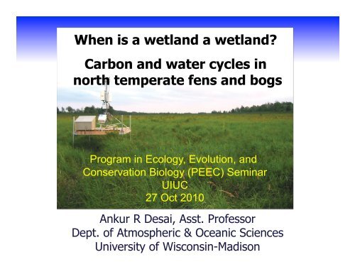
When is a wetl<strong>and</strong> a wetl<strong>and</strong>?<br />
<strong>Carbon</strong> <strong>and</strong> <strong>water</strong> <strong>cycles</strong> <strong>in</strong><br />
<strong>north</strong> <strong>temperate</strong> <strong>fens</strong> <strong>and</strong> <strong>bogs</strong><br />
Program <strong>in</strong> Ecology, Evolution, <strong>and</strong><br />
Conservation Biology (PEEC) Sem<strong>in</strong>ar<br />
UIUC<br />
27 Oct 2010<br />
Ankur R <strong>Desai</strong>, Asst. Professor<br />
Ankur <strong>Desai</strong>, Atmospheric & Oceanic Sci., UW-‐Madison <br />
Dept. of Atmospheric & Oceanic Sciences<br />
CEE 698: Susta<strong>in</strong>ability Pr<strong>in</strong>ciples, PracFces, <strong>and</strong> Paradoxes <br />
University of Feb Wiscons<strong>in</strong>-Madison<br />
9, 2010
Biogeo-what?<br />
• L<strong>and</strong> <strong>and</strong> ocean ecosystems have <br />
biophysical <strong>and</strong> biogeochemical <br />
dependences on the atmosphere <br />
– Biophysical – InteracFons of moisture, heat, <br />
solar radiaFon between ecosystems <strong>and</strong> <br />
atmosphere <br />
– Biogeochemical – Cycl<strong>in</strong>g of nutrients, <br />
especially carbon <strong>and</strong> nitrogen <br />
• As the atmosphere changes, both of these <br />
are chang<strong>in</strong>g <strong>in</strong> ecosystems! Lead<strong>in</strong>g to:
SURPRISE!
SURPRISE!<br />
• Ecosystems are generally evoluFonarily <br />
adapted to regional climate <strong>and</strong> its short-term<br />
variability <br />
• Expecta6ons of how these ecosystems <br />
respond to climate variaFon form the basis <br />
of ecosystem ecology <strong>and</strong> biogeochemistry <br />
• But: Surprises are likely given the complex <br />
<strong>in</strong>terplay between ecosystems <strong>and</strong> climate
SURPRISE!<br />
• Surprises are no fun for ecosystem <br />
management <br />
• But: It’s also how science progresses <br />
• And: We are likely enter<strong>in</strong>g an era where <br />
surprises will be more common. <br />
Why?
Our Era<br />
• From 1990-‐2005: <br />
– World Popula6on <strong>in</strong>creased 22% to <br />
~6,500,000,000 people <br />
– Global oil consump6on grew 25% to <br />
85,000,000 barrels per day <br />
– Gross World Product (GWP) grew 40% to <br />
$59,380,000,000,000 US dollars <br />
• PopulaFon doubl<strong>in</strong>g Fmes have <strong>in</strong>creased <br />
– 1850-‐1930, 80 years, 1-‐2 billion <br />
– 1930-‐1975, 45 years, 2-‐4 billion <br />
– 1975-‐2015, 40 years, 4-‐8 billion <br />
Source: UCAR
Why? CO 2 !<br />
385 ppm <br />
(2008) <br />
CO 2 (ppm) <br />
232 ppm <br />
Ice ages <br />
Years Before Present <br />
Source: Lüthi et al (2008), CDIAC, & Wikimedia Commons
S<strong>in</strong>ce 1990<br />
• Global annual CO 2 emissions grew 25% to <br />
27,000,000,000 tons of CO 2 <br />
• CO 2 <strong>in</strong> the atmosphere grew 10% to <br />
385 ppm <br />
• At current rates, CO 2 is likely to exceed <br />
500-‐950 ppm someFme this century <br />
• But: Rate of atmospheric CO 2 <strong>in</strong>crease is about <br />
half the rate of emissions <strong>in</strong>crease. Why?
Where Is The <strong>Carbon</strong> Go<strong>in</strong>g?<br />
Ecosystem <strong>Carbon</strong> S<strong>in</strong>k <br />
Houghton et al. (2007)
IPCC, 4 th AR, (2007) <br />
What’s The Big Deal?
IPCC AR4 (2007) <br />
The Big Deal
Friedl<strong>in</strong>gste<strong>in</strong> et al. (2005) <br />
A Small Problem
Houghton et al. (2007) <br />
<strong>Carbon</strong> Cycle
No Surprises Here<br />
• The befer we can reduce uncerta<strong>in</strong>ty of how <br />
ecosystem carbon/<strong>water</strong>/energy cycl<strong>in</strong>g responds <br />
to climate, the befer we can model future <br />
climate change <strong>and</strong> impacts <br />
• I will present a story to illustrate surprises of <br />
ecosystem responses to a chang<strong>in</strong>g climate based <br />
on research conducted by my lab <strong>and</strong> <br />
collaborators
• ExpectaFon: <br />
A Wetl<strong>and</strong> Story<br />
– Wetl<strong>and</strong>s store carbon under wet condiFons <br />
• Therefore: <br />
– RestoraFon of <strong>north</strong> <strong>temperate</strong> wetl<strong>and</strong>s <br />
should lead to <strong>in</strong>creased carbon sequestraFon
Wetl<strong>and</strong> <strong>Carbon</strong><br />
Boreal <strong>and</strong> subarcFc <br />
wetl<strong>and</strong>s conta<strong>in</strong> an <br />
esFmated 455 Pg <br />
soil carbon. <br />
This is up to 1/3 of <br />
total global soil <br />
carbon pool <br />
(Gorham, 1991) <br />
Mitra et al, 2005, Curr. Sci.
Biogeochemical Interactions<br />
CH CO 4 2<br />
CO 2<br />
CH 4<br />
Under<strong>water</strong><br />
(anoxic;<br />
anaerobic<br />
bacteria)<br />
Above <strong>water</strong><br />
(oxygenated;<br />
aerobic<br />
bacteria)
Biophysical Interactions<br />
Case 1: High <strong>water</strong> table<br />
High latent heat loss<br />
Case 2: Low <strong>water</strong> table<br />
High sensible heat loss<br />
Low sensible heat loss<br />
Low latent heat loss
Buffam et al. (2010) GCB <br />
Northern Highl<strong>and</strong>s
Buffam et al. (2010) GCB
A Tower
A Useful Tower
Many Useful Towers
A Useful Tower With Data
Methods<br />
• MulF-‐year flux tower Net Ecosystem Exchange (NEE) <br />
observed, quality controlled, gap-‐filled (<strong>Desai</strong> et al., 2005) <br />
• Rates of photosynthesis – Gross Primary Produc6on <br />
(GPP) <strong>and</strong> Ecosystem Respira6on (ER) derived from <br />
mov<strong>in</strong>g w<strong>in</strong>dow regression of NEE to environmental <br />
variables; NEE = ER-‐GPP (<strong>Desai</strong> et al., 2008) <br />
• Results compared to seasonal <strong>water</strong> table depth <br />
observaFons at each site (Sulman et al., submifed) <br />
• Six state-‐of-‐the-‐art ecosystem models parameterized <strong>and</strong> <br />
run at three sites with same meteorological forc<strong>in</strong>g <strong>and</strong> <br />
biometric <strong>in</strong>fo (Shroeder et al., <strong>in</strong> prep)
Wetl<strong>and</strong> <strong>Carbon</strong> Fluxes
Seasonal Variability
Interannual Variability
Natural Experiment
Decl<strong>in</strong><strong>in</strong>g Water Table
Trend?<br />
Sulman et al. (2009) Biogeosci.
SURPRISE!
Lakes Levels Are Dropp<strong>in</strong>g<br />
Stow et al. (2008)
Regional Climate Trends<br />
• StaFsFcally-‐<strong>in</strong>terpolated staFon data 1950-‐2006 <br />
WICCI (2009)
What Drives Water Table?<br />
• Water table elevaFon is driven by <br />
precipitaFon <strong>and</strong> evaporaFon <br />
Sulman et al. (2009) Biogeosci.
Evapotranspiration
Biophysical Interactions<br />
Case 1: High <strong>water</strong> table<br />
High latent heat loss<br />
Case 2: Low <strong>water</strong> table<br />
High sensible heat loss<br />
Low sensible heat loss<br />
Low latent heat loss
Energy Balance<br />
• Net radiation<br />
<strong>in</strong>creased due to<br />
<strong>in</strong>creas<strong>in</strong>g <strong>in</strong>com<strong>in</strong>g<br />
radiation <strong>and</strong><br />
decrease <strong>in</strong> albedo<br />
• Sensible heat flux<br />
<strong>in</strong>creased relative to<br />
latent heat flux<br />
• If these changes<br />
occur on a large<br />
scale, they can have<br />
significant effects on<br />
regional climate<br />
(Sampaio et al. 2007,<br />
Foley et al. 2003)<br />
Latent heat flux<br />
Sensible heat flux<br />
Net radiation<br />
Heat flux <strong>in</strong>to ground
A Wet Place
South Fork<br />
Wilson Flowage<br />
Lost Creek
A Bog
NEE-><br />
A Fen
NEE-><br />
• 27 site-‐years of data <br />
Some Wet Places<br />
Sulman et al. (2010) GRL
Mer Bleue<br />
Western Peatl<strong>and</strong>
Western Peatl<strong>and</strong> (Alberta)
NEE-><br />
S<strong>and</strong>hill Fen (Sask)
NEE-><br />
Mer Bleue (Ont)
NEE-><br />
Sulman et al. (2010) GRL
Sulman et al. (2010) GRL
Sulman et al. (2010) GRL
A Ha!<br />
• ProducFvity <strong>and</strong> decomposiFon have <br />
consistent, similar relaFonships to <strong>water</strong> <br />
table elevaFon <strong>in</strong> <strong>north</strong> <strong>temperate</strong> <br />
wetl<strong>and</strong>s <br />
• But: Fens <strong>and</strong> <strong>bogs</strong> respond <strong>in</strong> opposite <br />
fashion <br />
– relaFonship stronger <strong>in</strong> <strong>fens</strong> <br />
• The net effect is limited response of NEE to <br />
<strong>water</strong> table <strong>in</strong> both <strong>fens</strong> <strong>and</strong> <strong>bogs</strong> <br />
• Interannual <strong>and</strong> long-‐term may respond <br />
differently
Do Models Get This?<br />
• Six model, three site <strong>in</strong>tercomparison <br />
– Residuals = Modeled flux – Observed flux <br />
a) ER residuals <br />
Courtesy of N. Shroeder, UW <br />
b) GPP residuals
N. Schroeder,<br />
Senior Thesis<br />
Discrepancies
What’s Driv<strong>in</strong>g This?<br />
• AdaptaFon of plants to dry<strong>in</strong>g condiFons <br />
leads to <strong>in</strong>creases <strong>in</strong> <strong>water</strong> use efficiency, <br />
especially for <strong>fens</strong>, maybe?
Morals For Wetl<strong>and</strong>s<br />
• Wetl<strong>and</strong> carbon cycl<strong>in</strong>g is not a monotonic <br />
funcFon of <strong>water</strong> table <br />
– Fens may be more resilient to climate change <br />
than <strong>bogs</strong> <br />
• Plants adapt to change, but the Fmescale <br />
depends on the k<strong>in</strong>d of ecosystem <br />
Mesic forests? <br />
Temperate <strong>fens</strong>
From Sites to Regions<br />
• The fundamentals of ecology <strong>and</strong> <br />
micrometeorology have been mostly studied at <br />
the plot scale <br />
• The fundamentals of surface-‐atmosphere <br />
<strong>in</strong>teracFon <strong>in</strong>fluence on the climate systems have <br />
been mostly studied globally <br />
• Regions (l<strong>and</strong>scapes, <strong>water</strong>sheds, conFnents) are <br />
where climate-‐ecosystem <strong>in</strong>teracFons are least <br />
understood <strong>and</strong> likely to hold the most surprises <br />
– It’s also the relevant scale for ecosystem management
And Of The Region?<br />
• Northern Wiscons<strong>in</strong> is a mix of upl<strong>and</strong> <br />
forest (70%) <strong>and</strong> wetl<strong>and</strong> (30%) <br />
– Should regional CO 2 fluxes respond to <br />
hydrologic serng? <br />
• We can esFmate regional fluxes us<strong>in</strong>g <br />
– top-‐down by <strong>in</strong>verse or boundary layer budget <br />
approaches, or <br />
– bofom-‐up from forest <strong>in</strong>ventory or flux-‐tower <br />
opFmized ecosystem model<strong>in</strong>g.
• Bofom-‐up (scal<strong>in</strong>g) <br />
Methods<br />
– IFUSE – Interannual Flux-‐Tower Upscal<strong>in</strong>g Experiment <br />
• 12 regional flux towers categorized by l<strong>and</strong> cover <strong>and</strong> age are used to <br />
parameterize simple regional model us<strong>in</strong>g MCMC approach (<strong>Desai</strong> et <br />
al., 2008; <strong>in</strong> prep) <br />
– ED – Ecosystem Demography Model v1.5 <br />
• Height-‐<strong>and</strong>-‐age cohort succession model tuned to Forest Inventory <br />
<strong>and</strong> Analysis (FIA) data (<strong>Desai</strong> et al., 2007) <br />
• Top-‐down (atmospheric budgets) <br />
– EBL – Equilibrium Boundary Layer <br />
• 1-‐D boundary layer budget <strong>in</strong>ferred from WLEF 447-‐m tall tower CO 2 <br />
profile, NOAA mar<strong>in</strong>e CO 2 flask network, <strong>and</strong> NARR reanalysis <br />
subsidence rates (Helliker et al, 2004) <br />
– CT – <strong>Carbon</strong>Tracker v2009 <br />
• Global, nested-‐grid <strong>in</strong>verse model based on CASA surface model, <br />
global surface conFnuous <strong>and</strong> flask CO 2 network, <strong>and</strong> Ensemble <br />
Kalman Filter tracer-‐transport assimilaFon with TM5 w<strong>in</strong>ds (Peters et <br />
al., 2007)
Regional Flux<br />
• Magnitudes vary, but variability is similar <br />
<strong>Desai</strong> et al (2010) JGR-‐G
Regions <strong>and</strong> Water<br />
• Prior year <strong>water</strong> table strong <strong>in</strong>fluences <br />
anomalies <strong>in</strong> regional NEE <br />
<strong>Desai</strong> et al (2010) JGR-‐G
Morals: Noth<strong>in</strong>g Is Simple<br />
• <strong>Carbon</strong> <strong>and</strong> <strong>water</strong> cycl<strong>in</strong>g l<strong>in</strong>kages require close exam<strong>in</strong>aFon <strong>in</strong> <br />
ecosystem models <br />
– Moisture stress covaries with temperature <strong>and</strong> precipitaFon <br />
• Complex <strong>in</strong>terac6ons between the physical environment <strong>and</strong> all <br />
biological systems (e.g., <strong>in</strong>sects, microbes) should not be <br />
underesFmated – it’s where the surprises ouen hide <br />
– Lag effects, <strong>and</strong> posiFve/negaFve feedbacks can be complex <br />
– Models that <strong>in</strong>corporate, test, <strong>and</strong> verify these <strong>in</strong>teracFons can help us <br />
anFcipate surprises <br />
• Slow, steady rates of change allow us to anFcipate <strong>and</strong> react to <br />
surprises; rapid climate surprises are likely to exacerbate ecosystem <br />
surprises <br />
– Policies that slow climate change or destabilizaFon are wise with respect <br />
to m<strong>in</strong>imiz<strong>in</strong>g ecosystem disrupFon
Acknowledgements<br />
• <strong>Desai</strong> Ecometeorology Lab (flux.aos.wisc.edu): <br />
• Fund<strong>in</strong>g partners: UW Graduate school, NSF, <br />
UCAR, NOAA, USDA NRS, NASA, DOE, DOE NICCR, <br />
WI Focus on Energy
Acknowledgements<br />
• UW: Ben Sulman*, Nicole Schroeder*, Jonathan Thom* <br />
• SUNY-‐Buffalo: D. Scof Mackay <br />
• USFS: Nic Saliendra, Ron Teclaw, Dan Baumann <br />
• NASA GSFC: Bruce Cook <br />
• NOAA ESRL: Arlyn Andrews <br />
• UMN: Paul Bolstad <br />
• U. Lethbridge: Larry Flanagan <br />
• Trent U.: Peter Lafleur <br />
• UC-‐Berkeley: Oliver Sonnentag <br />
• Environment Canada: Alan Barr <br />
• U. Penn: Brent Helliker <br />
• Harvard: Paul Moorcrou