RW I:Discussion Papers - Rheinisch-Westfälisches Institut für ...

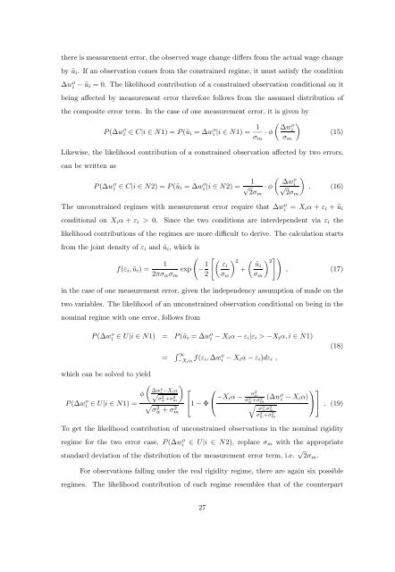
there is measurement error, the observed wage change differs from the actual wage change
by ũ i . If an observation comes from the constrained regime, it must satisfy the condition
∆wi o − ũ i = 0. The likelihood contribution of a constrained observation conditional on it
being affected by measurement error therefore follows from the assumed distribution of
the composite error term. In the case of one measurement error, it is given by
P (∆wi o ∈ C|i ∈ N1) = P (ũ i =∆wi o |i ∈ N1) = 1 ( ) ∆w
o
· φ i
σ m σ m
(15)
Likewise, the likelihood contribution of a constrained observation affected by two errors,
can be written as
P (∆wi o ∈ C|i ∈ N2) = P (ũ i =∆wi o |i ∈ N2) = √ 1 ( ) ∆w
o
· φ i √2σm . (16)
2σm
The unconstrained regimes with measurement error require that ∆w o i
= X i α + ε i +ũ i
conditional on X i α + ε i > 0. Since the two conditions are interdependent via ε i the
likelihood contributions of the regimes are more difficult to derive. The calculation starts
from the joint density of ε i and ũ i ,whichis
( [ (
1
f(ε i , ũ i )= exp − 1 ) 2 ( ) ]) 2 εi ũi
+
, (17)
2πσ w σ m 2 σ w σ m
in the case of one measurement error, given the independency assumption of made on the
two variables. The likelihood of an unconstrained observation conditional on being in the
nominal regime with one error, follows from
P (∆w o i ∈ U|i ∈ N1) = P (ũ i =∆w o i − X iα − ε i |ε i > −X i α, i ∈ N1)
= ∫ ∞
−X iα f(ε i, ∆w o i − X iα − ε i )dε i ,
(18)
which can be solved to yield
( )
∆wi φ
o−Xiα
⎡ ⎛
√
P (∆wi o σ 2 w +σm
∈ U|i ∈ N1) = √ 2 ⎣1 − Φ ⎝ −X iα −
σ 2 w + σm
2
σ2 w
σw 2 +σ2 m
√
σ 2 w σm
2
σw+σ 2 m
2
⎞⎤
(∆wi o − X iα)
⎠⎦ . (19)
To get the likelihood contribution of unconstrained observations in the nominal rigidity
regime for the two error case, P (∆wi
o ∈ U|i ∈ N2), replace σ m with the appropriate
standard deviation of the distribution of the measurement error term, i.e. √ 2σ m .
For observations falling under the real rigidity regime, there are again six possible
regimes.
The likelihood contribution of each regime resembles that of the counterpart
27