Gender Segregation and Gender Wage Differences during the Early ...

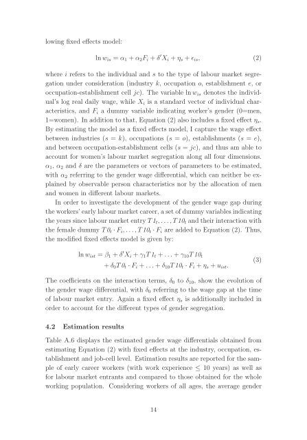
lowing fixed effects model:
ln w is = α 1 + α 2 F i + δ ′ X i + η s + ɛ is , (2)
where i refers to the individual and s to the type of labour market segregation
under consideration (industry k, occupation o, establishment e, or
occupation-establishment cell jc). The variable ln w is denotes the individual’s
log real daily wage, while X i is a standard vector of individual characteristics,
and F i a dummy variable indicating worker’s gender (0=men,
1=women). In addition to that, Equation (2) also includes a fixed effect η s .
By estimating the model as a fixed effects model, I capture the wage effect
between industries (s = k), occupations (s = o), establishments (s = e),
and between occupation-establishment cells (s = jc), and thus am able to
account for women’s labour market segregation along all four dimensions.
α 1 , α 2 and δ are the parameters or vectors of parameters to be estimated,
with α 2 referring to the gender wage differential, which can neither be explained
by observable person characteristics nor by the allocation of men
and women in different labour markets.
In order to investigate the development of the gender wage gap during
the workers’ early labour market career, a set of dummy variables indicating
the years since labour market entry T 1 t ,...,T10 t and their interaction with
the female dummy T 0 t · F i ,...,T10 t · F i are added to Equation (2). Thus,
the modified fixed effects model is given by:
ln w ist = β 1 + δ ′ X i + γ 1 T 1 t + ...+ γ 10 T 10 t
+ δ 0 T 0 t · F i + ...+ δ 10 T 10 t · F i + η s + u ist .
(3)
The coefficients on the interaction terms, δ 0 to δ 10 , show the evolution of
the gender wage differential, with δ 0 referring to the wage gap at the time
of labour market entry. Again a fixed effect η s is additionally included in
order to account for the different types of gender segregation.
4.2 Estimation results
Table A.6 displays the estimated gender wage differentials obtained from
estimating Equation (2) with fixed effects at the industry, occupation, establishment
and job-cell level. Estimation results are reported for the sample
of early career workers (with work experience ≤ 10years)aswellas
for labour market entrants and compared to those obtained for the whole
working population. Considering workers of all ages, the average gender
14