UNDERSTANDING DIGITAL TV - Ro.Ve.R. Laboratories S.p.A.

UNDERSTANDING DIGITAL TV
• Radio Frequency Measurements
• Propagation Effects
• Impedance & Matching
• SFN Networks and ECHOES
• Recommended Parameters & Limit Values

Dear Users,
This document does not intend to explain how Digital Terrestrial Television (DTT) works (there is another
Rover technical publication that clearly explains this called “An Introduction to DTT”), instead we hope
to provide practical, basic information about the transmission, propagation and reception issues
of digital television signals.
Above all we will look at how to improve reception in difficult locations and situations, especially in the
case of complex SFN networks, or in the presence of urban sources of electromagnetic noise.
May we remind you that in 99% of the cases, reception improves by working on the antenna ; unfortunately
no magic set top box or TV set currently exists.
We apologize in advance for any inaccuracies and invite you to notify us if you find any.
We hope you enjoy this and remind you that there is always business for competent and well equipped
professional antenna installers.
Some clarifications:
Each equipment manufacturer uses different names for the two BER’s, so we have decided to use the
acronyms employed by the British, who were the first to introduce a DVB-T network in Europe in 1998.
• bBER = where “b” stands for “before”, i.e. measured before Viterbi error correction.
This is also known as Pre BER or CBER.
• aBER = where “a” stands for “after”, i.e. measured after Viterbi error correction.
This is also known as Post BER or even VBER.
2

SUMMARY
6 Radio frequency spectrum
8 Average Channel power
10 RF Power measurement
12 DVB-T modulation
14 Performance indicators
16 Locking threshold
18 Before & After Viterbi error correction – Noise margin
20 Propagation effects
22 Reflection measurement examples (echoes)
24 Eliminating reflections
26 Antenna distance table
28 Reflections from the ground
30 The back to front antenna ratio
32 Impedance matching in distribution systems
34 SFN (Single Frequency Network)
36 ECHOES and guard interval
38 Measuring the network delay
40 Reducing echoes
42 The sum of the signals between two TX sites
44 Reception example between two TX sites
46 Modulation parameters and limit values
48 The Low limit for Q.E.F. Reception (Q.E.F. = Quasi Error Free)
50 Minimum Power and thresholds
52 EM fields and reception power
54 Correlation between MER & BER
56 Radioelectric reception quality
58 ITU Standard Procedure
60 Case Study - Microinterruptions
62 MER versus CARRIER.
64 The “signal stratification” effect
66 Impulse noise
68 Measuring impulse noise disturbances
70 Impulse noise interference spectrum
72 Mismatching and distribution
3

RADIO FREQUENCY MEASUREMENTS
RADIO FREQUENCY SPECTRUM
Analog, 1 program for each channel
You can see video, croma and audio
Digital, many programs for each channel
You cannot see the single contributions
4

The difference between the two signals is evident in that the digital signal is composed of thousands of
carriers, which give the impression of a continuous spectrum.
Each of these carriers is modulated in amplitude and phase separately and independently from the others
and brings with it a part of the total content of information. The user’s decoder must then interpret and
reassemble all the information, translating it into video signals and selecting the program required by
the user.
The difference that interests an installer is to measure the received “field”, it is a good idea to see if there
is a difference between an analog and digital situation to see how things are:
ANALOG - You measure the voltage of a single video carrier and express it in units. The most suitable
unit, used by almost everyone, is dBµV, ideal value: 60 dBµV level.
DIGITAL - This measures the power of the complete channel (Average Channel Power), calculating the
total power of each carrier (power, not voltage). The unit should be, logically, the milliWatt, or rather dBm
(0 dBm = 1 milliwatt), but if you still use dBµV for convenience, ideal value 50 dBµV.
5

RADIOFREQUENCY MEASUREMENTS
AVERAGE CHANNEL POWER
This is what you see when you
expand the spectrum of individual
carriers.
Digital signal: thousands of carriers exactly 6817
The power can only be the total amount of all of them
Delta f = space between the carriers
equal to approximately 1 KHz,
or to be precise 1116Hz
6

The function that allows you to find out the total power of all carriers is called the “Average Channel
Power”.
With professional analyzers you can choose different measurement modes, whereas in portable
analyzers this is fixed and always active for radiofrequency average power measurements.
Why is this strange way of measuring the power as a sum used?
Because every small carrier carries a piece of the entire channel and the quality of the signal depends on
all of the carriers.
It is possible, as we will see later, to also lose a part of the carriers, or have some at a very low level, but it
is the power of all the carriers that matters.
The meters on the market perform this measurement in various ways, they carry out the average
operation by splitting the spectrum into several parts and then calculate the total of the partial powers.
The result is the average power, called RMS (Root Mean Square value).
7

RADIOFREQUENCY MEASUREMENTS
RF POWER MEASUREMENT
The mains RF Power/Level units:
RF DIGITAL POWER RF ANALOG LEVEL
1mW = 0 dBm
1µV = 0 dBµV
0dBm = 108,7 dBµV 1mV = 60 dBµV
–58,7 dBm = 50 dBµV 1mV = 0dBmV (USA)
AVERAGE POWER IN DVB-T
• It is like powering an electric heater with
many small power linesDVB-T:
• Each line provides part of the energy
• The total heat is the total amount of all
lines contributions
8

The power of the digital signal is always measured in dBµV, but is different from analog:
ANALOG: Is the true voltage measured only for the peak of the video carrier and a certain amount
is required (about 1 millivolt, equal to 60 dBµV) to obtain a quality image, practically low level = low
quality, high level = high quality pictures.
DIGITAL: This is a measurement derived from the average power, obviously it is not possible to measure
8000 signal carriers individually. The result is however expressed in dBµV, a well known, familiar unit.
PLEASE NOTE:
The power of the received field is not so important in DVB-T, it only needs to have a required
minimum level that is about 40 dBµV (better 50 dBµV), after which it has no influence on the
quality. In fact, it is better to avoid levels that are too high and that could saturate and degrade
the set-top box and the quality of the signal received.
With numbers, as shown above, you can move very quickly from dBµV to dBm and vice versa: just add,
or remove the number 108.7, which is valid for 75 ohm systems. In the case of 50 ohms, the number
is 107. In all the meters you can select the unit of measurement you prefer: dBm or dBµV, or dVmV for
USA.
9

RADIOFREQUENCY MEASUREMENTS
DVB-T MODULATION
The carriers are modulated:
in Amplitude – vector length
in Phase – vector angle
Until the decoder detects that the vector falls
within the right square, there is no error and
reception is perfect.
Each carrier is modulated independently from the others.
Each carrier carries a piece of the total information.
The modulation is both for phase and amplitude, for example “64QAM” (the most used)
or “QPSK” or “16QAM” (or “256QAM” for DVB–T2)
10

The modulation is the same type for each carrier, but carries different pieces of binary information
and hence the amplitude and phase of the various carriers are different from each other. This gives a
confused representation of the spectrum, that appears to have a beard like the noise.
In fact it is very similar, because the information is random and randomly variable, so that the British have
coined the phrase “noise like signal”, which gives the idea of a completely unrecognizable signal within
the spectrum.
The noise picked up by the antenna, or interference, makes the carrier’s vector moving randomly within
its square; if the noise increases the amplitude, it can throw it out and then there will be an error and the
video image will become unrecognizable suddenly and without notice.
Instead, in an analog signal, the noise, or interference, has a progressive action and is immediately
visible on the signal.
In the case of a digital signal, by observing the spectrum and the received power, it is not clear when the
various carriers are received correctly, because you do not know how much noise disturbance there is,
and how it affects the reception.
Later you will see what to do when working on headends and antenna pointing, in order to obtain the
best signal and work out how to measure the signal quality.
11

RADIOFREQUENCY MEASUREMENTS
PERFORMANCE INDICATORS
Some errors =
Only a few dots are outside the right
square
MER is reasonable
Few errors - BER worsens
The MER shows bad positioning of the vectors
The BER tells you the percentage of bit errors
Possible error =
The dots are scattered but not
outside the square
High MER, good BER
No error =
Excellent MER and BER
12

We know that signals can be “polluted” by noise or other interference.
These “uninvited guests” are often present and are added randomly, from time to time, to the vectors of
carriers and alter their position, making it difficult to recognize groups of bits from the decoder.
It is not possible to predict the magnitude of the noise disturbance, which is constantly changing, but
you can expect to constantly commit errors in the recognition of the bits.
To counteract this behavior the FEC (Forward Error Correction) mechanism has been introduced at the
cost of reducing transmission capacity, it allows the correction of errors - of course there are limits to the
correction capability.
The measurement is carried out by counting the errors: various instruments record, using a counter, up
to 999 errors and this is why the measurement takes a lot of time.
IMPORTANT:
Remember that, even in the presence of errors, the signal is decoded correctly, maintaining
the highest quality, so a method is required to determine the quality of the reception system.
Practically find out how many dB we can increase the noise or interference, without affecting the
quality of the received information this is called “Threshold Point”.
13

RADIOFREQUENCY MEASUREMENTS
LOCKING THRESHOLD
DIGITAL
More noise, or interference,
Up to the threshold,
THEN CRASH!!
picture
quality
good
average
decoding
margin
poor
signal intensity
ANALOG
More noise, or interference,
less quality
PICTURES WORSEN SMOOTHLY
BUT IT CAN BE SEEN
• DVB-T implements powerful error correction (FEC)
• Even though there is interference, up to a point, it is corrected
• To understand how much margin is left before a crash there is the:
MER (modulation error ratio)
14

The DVB-T signal has this behavious, which has both advantages and disadvantages:
Advantages:
1. Obviously the quality is always high, even in the presence of noise disturbances.
2. The signal power is no longer critical, you do not have to worry about constantly bringing it to the
maximum power, the quality is always high, regardless of the signal power strength.
3. The minimum power required is much lower than the level required for analog.
Disadvantages:
1. In the case of analog bad reception, if you could not do anything else, you could build the best
reception system at its limit, warning the customer that he has to settle for poor quality.
2. In DVB-T this cannot be done: if there is increased noise, the decoder remains completely unlocked
(threshold phenomenon).
3. Interruptions of a few seconds and “macroblocks” are much more disturbing in a momentary drop
in analog quality, which resumes immediately.
15

RADIOFREQUENCY MEASUREMENTS
BEFORE & AFTER VITERBI ERROR
CORRECTION - NOISE MARGIN
DEMODULATOR
1st ERROR CORRECTION
VITERBI
2nd ERROR CORRECTION
REED SOLOMON
MPEG DECODER
bBER
aBER
• Absolutely minimum bBER and MER: bBER=2x10 –2 and a MER of approx. 20 dB
(You must remain above these limit values, 6 dB noise margin (with 64QAM)
• Viterbi reduces errors until 2 x 10 –4 (after Viterbi aBER)
• Reed Salomon corrects what is left up to BER 1 x 10 –11
• This is QEF (quasi error free) – an error event statistically visible every 30 minutes
16

Here you can see a schematic block of the structure of a DVB-T set top box, where error correction is
done in two stages, as is carried out in TV and SAT set top boxes.
The Viterbi circuit is common to all types of digital broadcasting and clears up most of the errors and
adapts the system for the Reed Solomon error correction.
What happens is that the number of errors at the decoder input is highly variable, and after Viterbi error
correction it is much lower and more consistent.
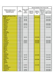
In the picture on page 18 you can see the error limits tolerated by the system, but as we already said,
the limits must be much higher and if you want an acceptable and stable quality you must have some
Margin (usually the Noise Margin in DVB-T must be 6 dB).
IMPORTANT:
The real innovation in the work of installation and development of an antenna system for digital
signals (unlike analog), lies in the noise margin concept, to be respected for all digital systems,
including cable and satellite distribution. Since the minimum values ​of various parameters to be
analyzed differs between the various systems satellite, terrestrial and cable (see table on page 2), some
meters automatically provide the signal quality FAIL–MARG–PASS, and this greatly simplifies the job.
17

PROPAGATION EFFECTS
The reflected signal delays because
it has to travel a longer distance
DELAYED BUT SYNCHRONOUS
If the two transmitters are “synchronous”,
for the reception
IT IS LIKE HAVING A REFLECTION
• In analog the reflection causes a double image
• DVB-T does not suffer at all from signal reflections
• A degrading exists, but it does not have any effect on the picture quality
18

When it is said that a DVB-T system is immune to reflections, this is not completely true.
The reflected signal acts exactly like a noise disturbance that lowers the MER and raises the BER; this
causes errors in the received signal, but we know that the system is perfectly capable of defending itself,
especially when you have an adequate noise margin.
At this point we will introduce a new topic and a new source of noise disturbance and an operational
difficulty arises immediately:
In ANALOG, you can distinguish immediately, by looking at the picture, which type of noise
disturbance you are facing. It is clear that the double image is produced by a reflection, while the
noise causes the snow effect, compression crushes synchronisms etc.
In DIGITAL, any kind of interference and reflections generate the same effect, that consists of a
lowering of the MER and BER deterioration.
We will see later an almost infallible method to detect the presence of reflections and to know how
to act.
Of course it is very important to discover what is causing the interference, because the actions
required to eliminate it can be different according to the type you are experiencing.
19

PROPAGATION EFFECTS
REFLECTION MEASUREMENT EXAMPLES
(ECHOES)
• 3.5 MHz approx.
• The delay will be:
1/3.5 = 0.28 microsec.
• 80 meters approx.
20
TX signal
power
difference
[dB]
Maximums
[dB]
Spectrum Ripple
Minimums
[dB]
Relationship between Frequency Interval in MHz between two power dips in the spectrum and
related delay in microseconds
These are inverse operations: Delay = 1/ (frequency interval)
(In the spectrum you can only see short delays from close obstacles).
Total,
peak-peak
[dB]
0 +6 – –
1 +5.5 –19.3 24.8
3 +4.6 –10.7 15.3
10 +2.4 –3.3 5.7
20 +0.8 –0.9 1.7

Let us assume that the electromagnetic signals (light and electromagnetic radio
waves, but also X-rays) propagate at the speed of light, in other words:
• 300 meters per microsecond.
• 3.3 microseconds to travel one kilometer.
• 224 microseconds to travel 67 kilometers.
Of course, everything comes from the speed of light of 300,000 kilometers per second.
Obstacles, that act as mirrors, send to the receiving antenna a signal that is the same as the signal
required, but this signal is delayed and attenuated. With an analog signal you will see a double image
on the screen. If you have a large screen of about 50 cm, the shift is: as many µS as there are cm of
displacement between the two images.
Knowing this, sometimes you can derive the distance of the point of reflection.
In DVB-T systems you cannot see the double image, but the spectrum display shows dips in the spectrum
(ripple).
This can be explained considering that the signals become unphased along the way and the delay varies
with frequency, resulting that in some areas of the spectrum there are signal reinforcements in some
areas signal drops.
Signals are equal to each other, the spectrum goes close to zero in the gaps and to +6 dB in the peaks.
We will show you how instruments can provide easy and accurate systems to obtain the amplitude and
distance of the reflections (ECHOES).
21

PROPAGATION EFFECTS
ELIMINATING REFLECTIONS
Antennas connected
with two cables of
equal length and a
combiner
Desired signal
Distance D
22
Disturbing signal
Optimum distance:
D = λ/(2xsenθ)
λ = wavelength

We will illustrate a laborious, but very effective, method to reduce the reflections that interfere with the
desired signal.
Let’s assume that with this system, whose success depends on the quality of the mechanical design, you
can decrease the interference level by 15 dB and in some cases, with professional antennas, by up to 20
dB.
It is essential that there is the presence of only one interference source, from a known direction and that
you are sure that the signal level does not vary much, undermining the job done.
Keep in mind that disturbing signals can vary by 20 or more decibels, with different weather conditions,
and the more so if they come from far away or if they travel across lakes or seas.
The system works because it makes the disturbing signal take a longer path of exactly half a wavelength,
before reaching antenna 1, so that it reaches the combiner with 180° phase rotation (anti phase). The
desired signal, however, always arrives in phase, along the same route to reach the antennas, then to the
combiner.
Result reached: more than 3 dB for the desired signal and 15 dB attenuation of the noise
disturbance.
With analog it is difficult to eliminate a reflection entirely, whereas with DVB-T it is easier to gain the
margin required to achieve good stability.
23

PROPAGATION EFFECTS
ANTENNA
DISTANCE TABLE
CHART: DISTANCES BETWEEN ANTENNAS ANTIREFLECTION
ANGLE
FREQUENCY IN MHz
DEGREES
Distances in meters
The values are critical, use the table only for the first
approximation, then adjust the distance until you
reach the maximum spectrum flatness
24

This chart is useful, even if it does not cover all frequencies and angles.
The values ​are calculated exactly, but you must carry out an experimental set-up, because you will never
exactly know which direction a signal is coming from.
It is especially useful if you want to see if a mechanical system is physically possible, given that sometimes
very large distances are involved.
If the distances are too small and the antennas are touching, just double the distance to obtain an
acceptable one.
The system works very well, especially in the case of reflections from the terrestrial surface, with antennas
fixed to a mast, one below the other.
This is often found near lakes, or in the case of sea travel, but in these cases the angles are small.
A good test is to vary the height of the receiving antenna. If this causes ripples in the spectrum, that vary
with height, then you can be certain that there is a reflection from the ground.
If the depth of the ripples is considerable, or part of the spectrum is missing, then you must be careful,
especially if the reflection takes place on water, given the inherent variability of the situation, basically it
changes often during the day and night.
25

PROPAGATION EFFECTS
REFLECTIONS FROM THE GROUND
At the point of reflection the incoming and outgoing angles are the same
If you vary the antenna position, the point of reflection changes!
26

Another situation where the antenna is shown to be the most important component for improving
reception is that of “reflections from the ground.” This system is useful for many towns located close to
large water surfaces, e.g. lakes or the sea, where reflections are strong and there are rather large angles,
given the short distances from the transmitters. In the case of very distant transmitters, however, the
angles are small and force long distances between the antennas. With professional antenna towers, you
can make systems work with distances in the order of 30 or 40 meters.
For example, a transmitter 1000 meters high at a distance of 10 km, is seen under an angle of about 5
degrees, which requires a distance of about 3 meters.
To see if there are reflections from the ground, measure the field and slowly vary the height of the
antenna. If you notice any dB variations, there are sure to be ground reflections (see picture above).
In this case positioning the antenna at the maximum point may not be enough to solve the problem,
because reflection conditions vary with weather conditions. It is not the reflected signal’s change in
amplitude that causes problems, but the variation of the point and the reflection phase, which takes you
from a maximum to a minimum point.
A very effective system is to shield the antenna from the reflected beam, by lowering it and using
the roof of buildings to shield it from the reflected signal.
27

PROPAGATION EFFECTS
THE BACK TO FRONT ANTENNA RATIO
“L” Any length
To the Set Top Box
“L” Any length + λ/4
From the front the signals are in phase and the anticipation is compensated by the cable
From the back the lower antenna is delayed λ/4 and the cable delays again λ/4.
The signals reach the combiner with 180° phase rotation (ANTIPHASE) and cancel the other signals.
28

The back to front antenna ratio is the difference, expressed in dB, between the antenna’s response to
signals coming from the two directions, front and back.
In the case of SFN networks, on flat ground, where there are no natural barriers to prevent propagation
from very distant and powerful transmitters, there are wide areas that receive signals from the back of
the antenna.
The proposed system is very useful and practical, given the small distances between the antennas.
It may be convenient to mount two small antennas, instead of trying to find an expensive, huge aerial
with a very high back/front antenna ratio. Large antennas are very difficult to find and almost always
cause problems when you are forced to move the antenna across the mast, that, being metal, in many
cases distorts the antenna diagram.
Our only warning: the distance between the antennas must be exactly one quarter of the
wavelength, while the length of the longer cable should be calculated as follows:
Increased cable length = length of quarter-wave multiplied by speed factor of the cable.
This factor is provided by all manufacturers: for compact insulation (polyethylene) it is 0.66, whereas for
expanded cable it is around 0.87.
29

IMPEDANCE MATCHING
IN THE DISTRIBUTION SYSTEMS
GOOD MATCHING
Head end
Amplifier
In DVB-T systems you can clearly see the
effects of impedance mismatching
BAD MATCHING
Head end
Amplifier
75 Ohm load
There are no waves
(ripple)
There are no waves
(ripple)
1. The terminating resistor is
missing
2. A reflected wave is generated
that returns to the top
3. This behaves like a reflection
captured by an antenna
4. The result:
VISIBLE WAVES (ripple)
UNPREDICTABLE RESULTS
HUGE DIFFERENCES IN LEVEL
30

The reflections caused by a mismatch are the same as those caused by a
reflecting obstacle in the antenna.
The difference is that distribution lines can be adapted, thus producing an excellent result, whereas
when it comes from the antenna ... sometimes you can not do anything.
The return wave is added or subtracted from the direct wave according to the positions where the two
waves are in phase or in antiphase.
There are two ways to express the mismatch:
1. RL (Return Loss):
expressed in dB, showing how much the reflected wave is attenuated compared to the transmitting
wave and the higher it is the better the matching.
It should be higher than 10–12 dB.
2. VSWR (Voltage Standing Wave Ratio):
expressed as a linear number, this is the ratio between the maximum and minimum voltages
along the cable. It should be lower than 1.4–1.2.
The best way to measure the VSWR is to use a reflectometer, but it can be observed if the distribution
network alters the flatness of the spectrum, changing the shape compared to the one received from the
antenna.
A noise generator is very useful to easily test all distribution systems, because it shows all the TV or SAT
bandwidth on a single screen.
In countries such as Spain, this test is required by law, see “ICT” regulations.
31

SFN (Single Frequency Network)
Urban area of
coverage
Extra-urban area of
coverage
32
The reflected signal is delayed, but absolutely synchronous
The DVB–T system may tolerate delayed reflections up to 224 µSeconds, according to the
modulation parameters
It is possible to run a network of synchronous transmitters all with the same frequency

Since the system is immune to reflections (within the limits), a network of completely synchronous
transmitters can be put into action and already operating in some countries like Spain and Italy.
All you have to do is transmit the same bit at the same time and at the same frequency.
Achieving this goal is very complicated and expensive; completely synchronous digital distribution
networks are required, many transposers will need to be converted into transmitters. Finally an accurate
frequency reference at all sites must be guaranteed.
It is sufficient to say, for example, that the required accuracy is about 1 Hz for the frequency and few
nanoseconds for the timing.
The following points clarify the topic:
1. A reflected signal, is still tolerable however far it is, but it must be at least 20 dB below the level of
the desired signal, and does not reduce the margin too much (basically it is like any kind of noise).
2. If, however, the delay is below a certain limit, which depends on the transmission parameters, you
could even tolerate a reflected signal at the same level as the one received.
3. It is a good idea to keep it about 6 dB lower than required, to make sure that it is safe from random
deterioration and variations.
33

SFN (Single Frequency Network)
ECHOES AND GUARD INTERVAL
direct
path
+
echo
=
signal
received
symbol N
symbol N
intersymbolic
interference
symbol N+1
symbol N+1
intrasymbolic
interference
The echo is an attenuated
and delayed copy of the
desired signal
A downtime is inserted
called the
GUARD INTERVAL
• If the reflections fall in the guard interval, they do not generate errors (the decoder simply
throws away all the wrong information in the guard interval)
• As soon as they fall outside the guard interval, the decoder see them as interference and ...
this is pain!
34

Operation is based on being able to delete the wrong part of the information from the delayed reflection.
It’s as if, trying to talk in the presence of an echo, you could eliminate the first part of the pronounced
syllables. An echo, if not too delayed, only ruins the first part of the syllable next to the one just
pronounced. Of course you would need a whole synchronized system to be able to guess where to cut
off.
To function properly, the so-called SFN Single Frequency Network, needs transmitters with power that
is calibrated and not too high, so as not to get too far away, where it would have a delay, against to local
transmitters, outside the maximum distance allowed.
The maximum delay is called the GI, Guard Interval, and is 224 microseconds for SFN mode (8k carriers).
Often transmitters have intentional delays, inserted to adjust the arrival times of signals in the area, but
it is not always possible to meet all the requirements in difficult territories.
In these cases, an installer should know how to search for and measure the various signals arriving at the
antenna and to point it with accuracy in order to eliminate the signals that arrive with too many delays.
35

SFN (Single Frequency Network)
MEASURING THE NETWORK DELAY
• Measure the delay time
between reflections
• Each received signal is
shown as a vertical bar
• Horizontally you can
read the delay in
microseconds, or the
distance in km
Example of good reception in SFN
networks. There are two echoes,
but they are inside the guard time
The “PRE ECHO” is shown here
A weak reflection that arrives first
Sometimes this can cause problems for
some decoders
Example of bad reception in SFN
networks. There are two echoes
outside the guard interval.
36

Nearly every instrument has an SFN mode and many of them can show a graph like the one shown in
the figure on page 38, where the various incoming signals are shown as lines, or vertical bars (remember
that all the signals have the same frequency).
What you see from the SFN ECHOES screen:
1. The horizontal axis allows you to read the delays between the various signals. In general, the
instrument takes the best signal and places it at zero and below each vertical bar you can read the
delay of the individual signals.
2. The amplitude of each signal, with the indications given in dB on the vertical axis, are shown on the
left scale.
3. Typically there is a coloured area (in these cases the green area), that represents the guard interval,
so you can see at a glance if a signal is too strong and falls outside the guard interval.
IMPORTANT:
Orientation of the receiving antenna must be optimized, to look mainly where you can make one
signal stronger than the others and reduce the others that fall outside the guard interval.
It is worth remembering that it is better to reduce the ECHOES, especially those outside the GI,
rather than just searching for the maximum power of the signal received.
37

SFN (Single Frequency Network)
REDUCING ECHOES
&
MAX distance
• The signals travel at the speed of light
• They go at 300.000 km per second, 300 metres in a microsecond
• Roughly 3.3 microseconds per kilometer
• Map in hand, you know immediately if you are receiving a TX in or out of the guard interval
distance
38

Here are a number of rules to improve management of SFN reception:
1. It is inevitable that when covering vast territory some areas will be in the shade; with digital DVB-T
is more a problem of coexistence of SFN signals.
2. Even when the arrival times of signals are contained within the guard interval, it is dangerous to
operate systems with SFN signals at the same level. To obtain an adequate MER and BER margin
echoes should be at least 10 dB below the main signal.
3. There could, in theory, be a situation in which two antenna signals arrive at the same level and with
the same delay, resulting in no pictures or what is received is extremely unstable.
4. Use directional antennas and take a close look at the SFN ECHOES screen, to check the best position
of the antenna (for example, try to shield in the direction of unwanted incoming ECHOES).
5. Be very careful to combine 2 or more antennas: an antenna pointed in one direction will inevitably
pick up signals from another direction, causing, unwanted reflections (ECHOES).
6. Contributions outside the guard interval are considered interferent and must be reduced by at
least 25 dB.
IMPORTANT:
Orientation of the receiving antenna must be optimized, to look mainly where you can make one
signal stronger than the others and reduce the others that fall outside the guard interval.
It is worth remembering that it is better to reduce the ECHOES, especially those outside the GI,
rather than just searching for the maximum power of the signal received.
39

SFN (Single Frequency Network)
THE SUM OF THE SIGNALS BETWEEN TWO TX SITES
In the darker areas you
have the phase sum:
6 dB increase
Along these lines you can see
the delay in micro-seconds (50
µS each line)
µS µS
TX1
TX2
40

This picture shows an example of an SFN network on a perfectly flat area, with no natural obstacles, and
where there are two SFN transmitters.
When exploring an area, you will find locations where signals are added and others where they are
detracted, due to phase variations and depending on the distance between the transmitters.
In areas, where the received fields from two sites are identical or very similar, variations are very strong.
There are points where the signal goes to zero and points where it increases 6 dB, at a distance of about
half a wavelength, because at every half wavelength there is a phase invertion:
Wavelength λ = 300/frequency in MHz
When you move away from a TX site, its signals become weaker in comparison to the other TX, making
phase shift less strong and with a flatter spectrum, because the phase shifts depend on the frequency
and distance. Single Frequency Networks work only while delays are kept within the guard interval.
The diagram shows an area of about 100 km, where delay in µS is constant along the curves: this delay
is shown for each curve.
We must ensure that in the area, where the delay exceeds the guard interval, you receive signals from
only one TX, using antennas with a good back to front antenna ratio, as already seen and shielding it
from the other TX.
41

SFN (Single Frequency Network)
RECEPTION EXAMPLE BETWEEN TWO TX SITES
300µS
250µS
200µS
150µS
100µS
42
Along the lines signals are received from two TX sites with the same delay
50µS

As an example, we have superimposed a network of curves, with a constant level, onto a geographical
map of the Padana Valley in North-West Italy. Here there is an SFN network, designed and built by the
Italian broadcasting company Rai Way, which implements a few sites with high power transmitters that
cover a very wide area.
You can see that the distance between the TX sites of Mount Penice and Mount Eremo is so far that the
delay exceeds the guard interval. To the east of Mount Penice there is Mount Venda, another high power
TX site, and this is also in SFN with TX sites covering the regions of Friuli and Emilia Romagna, North East
of Italy.
In cases like these it is very difficult to make the delays fall within the guard interval by inserting artificial
delays at the various sites, because what you gain in one direction, you lose in the other.
However natural obstacles can help to prevent propagation beyond a certain distance (see the hills
to the east of Turin) as well as the careful design of antenna diagrams and the calibration of power in
transmission.
The directivity of the receiving antennas is of fundamental importance.
International planning bodies, who dictate broadcasting regulations, have established that a basic
antenna should have an attenuation of 10 dB for signals from an angle exceeding 25 degrees and about
15 dB for cross-polarization.
43

MODULATION PARAMETERS AND LIMIT VALUES
Net bit rate (Mbit/s)
FEC
G.I.
Most
used in
Italy
44
Showing relation between: transport capacity with various
Modulations, F.E.C. and Guard Interval

The diagram clearly shows the transport capacity of the DVB-T transmission system, with various
modulation layouts (constellations).
They range from a capacity of about 7 Mbit / second to a capacity of about 35 Mbits / second, which
means being able to transmit from 1 to 4 or 5 programs, some in high definition.
As you can see what you get in transmission capacity, you pay in terms of signal robustness and
vice versa..
If you want to manage an SFN network, you need to dedicate part of the capacity to the guard interval
and FEC, as shown by the length of the histograms.
The system chosen is shown, which combines a good ability to correct errors, given the high FEC, and
a good Bit Rate capacity; this is accomplished by using 64 QAM modulation, which needs an adequate
margin of MER and BER, as we shall see next.
45

Parameters and limit values
THE LOW LIMIT FOR Q.E.F. RECEPTION
QEF = Quasi Error Free
Most used in Italy
Minimum Required C/N (dB)
46
Showing relation between: Carrier to Noise and Modulation
parameters to obtain Q.E.F.
Channel with lots of ECHOES
---RAYLEIGH---
Optical visibility and some (few)
ECHOES
---RICE---
Basic channel, degraded only
by noise
---GAUSSIAN---

To obtain minimum reception stability, there should be the following conditions:
QEF - Quasi Error Free; Reception “almost” free from error.
Do not allow yourself to be misled by the word “almost”. Its meaning is clear: you must not tolerate
more than one error per hour in the demodulated digital signal.
This translates into a maximum number of errors tolerated at the antenna, which can reach up to bBER
1 x 10 -2 , i.e one bit error out of the 100 transmitted.
In normal reception conditions, usually the main source of degradation is thermic noise, in other words
the interference that causes “the snow effect” in analog systems.
In the case of satellite reception, this is the only condition you could find because there are no obstacles
along the way that could cause reflections and no interference, except for very few cases.
So for DVB-T reception the main problem is still thermic noise. In the diagram you can see, from
the height of the bars, the C/N - signal to noise ratio required for reception at the limit of the locking
threshold, in other words, without any Noise Margin, but in QEF conditions, this means that for good
and stable reception you must add some dB.
It shows three kinds of reception (Rayleigh–Rice–Gaussian), using the names of famous scientists, who
studied the statistics used to find these values​.
Since no one can accurately predict the electromagnetic fields found at the home of each user, field
predictions have been carried out, that adhere to International standards and that can effectively
calculate on a 200 X 200 meter grid.
47

Parameters and limit values
MINIMUM POWER & THRESHOLDS
Correction for
time variation
Correction for
space variation
C/N
QEF
(Quasi Error Free)
Minimum level
Noise level
The received fields are not checked in all points of the served area.
Statistic corrections are inserted against the signal variations in space and time.
48

These predictions are verified when the transmitters are activated, making point by point measurements
(once again following the appropriate regulations).
Due to the particular behaviour of DVB-T, it can generate interruptions of service instead of reducing the
quality, the field is increased to ensure the statistical coverage of all users.
A similar increase was made ​to prevent variations from interfering signals, this is very dangerous because
interferences often fall outside the guard interval and some times they are very strong, in the case of
random propagation conditions.
For this reason a Power Margin must be guaranteed, with a minimum of 6 to 10 dB more than
minimum sensitivity.
From laboratory tests, carried out on commercial decoders, it was concluded that almost all begin to
decode QEF at about 29 dBµV power! This is a very low value, but corrections must be added. As
explained next, you will see that you get about 39 dBµV as the absolute minimum, but it is better to
keep it around 49 dBµV.
49

Parameters and limit values
EM FIELDS AND RECEPTION POWER
Example at 500 MHz:
Antenna: 10 dB gain
Level measured: 41 dBµV
1. Read the antenna factor..... 14.5 dB
2. Add the level ....................... 41.0
3. Total ..................................... 56.5 dBµVm
Antenna factor calculated for an antenna
with 10 dB gain
50

The electromagnetic field is measured in dBµV/m
The received power is measured in dBµV.
Both of these measurement units make the various calculations very easy when you need to
find out the various levels in a distribution system: just add or subtract gains or, respectively,
attenuations encountered by the signal along its path.
In fact, all you need is a table showing the minimum values required by the various distribution systems,
then by adding the cable attenuations and subtracting the amplification gain, expressed in dB, you can
find out the value ​of the power signal, always expressed in dBµV.
The antenna factor is useful because the planning values ​are given in terms of electromagnetic
field, i.e. in dBµV/m.
The antenna installer, who knows the antenna gain or uses a graph similar to the one shown, is able to
predict with sufficient accuracy, the signal power available at the decoder input, or at the measuring
instrument input.
In summary: the amount in dBµV/m indicates “how much field falls on a roof”, while the antenna factor
tells us how much “electromagnetic rain ” you can capture with your antenna.
NOTE: For antennas with a gain higher than 10 dB, subtract from the reading on the graph, the difference
in gain.
E.g.: F = 470 MHz; antenna G = 13.50 dB, antenna F reads 14 dB
You must subtract: (13.50 - 10) = 3.5, then antenna F = 10.5 dB,
viceversa, if the antenna gains less than 10 dB, you must add the difference.
51

Parameters and limit values
CORRELATION BETWEEN MER & BER
These measurement dots
clearly show that in many cases
you can have a good MER and a
bad BER
15 20 25 30 35
Results of a series of measurements carried out after activating an experimental SFN network in 1999.
52

Even if the MER is a good indicator of quality, there are some important exceptions.
There are cases that complicate operation and create confusion due to the loss of coherence between
data, which seem not any more comparable. You could start by saying that, only in the presence of pure
thermal noise, the MER and C/N almost coincide.
The BER before Viterbi error correction (bBER) is an index that can be used to determine the overall
quality of a signal, but sometimes the best MER does not correspond to the good BER, or that this
does not improve even if the MER has very high values. This is normal behavior, and it was mentioned
earlier. The graph clear shows that the two parameters are not consistent, which is evident in the case of
impulsive interferences or pre-echoes.
You must always carry out both measurements and remember that quality is essentially
dependent on the BER. You must make any adjustment to the system, e.g. to the orientation
of the antenna or any other modification, but you must check the MER and BER and pay less
attention to the received power. Use the MER as an index to check the quality of amplifiers and
especially converters, based on the deterioration introduced between input and output of the
various elements of the systems.
N.B. Because each instrument manufacturer names the two BER in a different way, we have decided to
use the acronyms used by the British, who were the first to introduce a DVB-T network in Europe in 1998.
• bBER = “b” means “before”, i.e. measured before Viterbi error correction and is also called Pre BER or
CBER.
• aBER =
“a” means “after”, i.e. measured after Viterbi error correction and is also called Post BER or
even VBER.
53

RADIOELECTRIC RECEPTION QUALITY
SERVICE
LEVEL
GOOD
RECEPTION
more than acceptable
reliable
Suggested acceptable limit
unreliable
does not decode!
BAD
RECEPTION
With DVB-T you should distinguish between radioelectric reception quality and video quality.
The main parametrs are: bBER and channel power
54

The diagram shows once again the threshold behavior of DVB-T and is the base to measure the quality
of a signal or for a complete distribution system.
The aim is to carry out a measurement that says, with certainty, how far we are from the threshold,
which marks the boundary between unstable and unsatisfactory reception and a situation which gets
better and better, until you reach the optimum.
Obviously, in this step, all reception parameters raising on values ​that get better and better, from dark
red to dark green.
After the necessary measurements have been carried out, results can be put in a graph, and then you
can see the level of quality of service provided to the user.
Do not ever confuse the five levels of quality with analog ones, where a number from 1 to 5 indicated
“how the picture was seen”: starting from unacceptable = grade 1, to a perfect picture = grade 5.
DVB-T gives you a number that indicates the quality, which is not connected in any way with the quality
of the video picture, which remains the same when the decoder begins to lock without interruptions.
Instead, quality is linked to the stability over time: interference, noise, echoes and so on are highly
variable over time, so we have to make sure we reach the best measurement parameters over the
minimum allowed.
55

Radioelectric quality
ITU STANDARD PROCEDURE
Power
received
increasing
in the
direction of
the arrow
Over 40
Table of values to determine the quality
4x10 -2
2x10 -3
2x10 -4
better than 2x10 -4
bBER improves in the direction of the arrow
56
KEY:
bBER = before Viterbi (measured before Viterbi error
correction) also known as C BER
aBER = after Viterbi (measured after Viterbi error
correction) also known as V BER
CBER, or bBER before Viterbi error correction, is the most
important parameter.
The after Viterbi error correction Ber (aBER) must be better than
2x10-4, the minimum limit for the decoder to lock.
Many meters automatically supply a quality index and this
makes work much easier.

This table is calculated for systems with a FEC equal to 2 / 3, but in
practice it can be considered valid in all cases.
The parameters used for evaluation are the bBER and the Power of the received channel, practice has
proved the validity of this measurement system.
A similar table is used when we predict the quality of reception in the design phase, using the field in
dBµV/m.
The values ​shown can be used as an approximation, the absolute level of quality is not so
important, but the most important thing is to have an adequate Noise Margin.
Some meters, currently available on the market, have built-in software that calculates the quality and
expresses it very simply using three levels: Pass, Marginal, Fail.
This is all that is required for a quick evaluation of the reception conditions: in practice the first step of
the scale has been omitted, but this has virtually no importance. In difficult reception cases, or with
signals at the limit of decoding, determining the quality becomes very difficult and useless.
In very difficult cases it makes no sense to measure the quality, you should seek only the best reception
possible and this can only be done by measuring the various parameters and trying to maximize them
with the antenna.
In these cases, any improvement is determined by the quality of the antenna and its position, as described
previously.
The antenna is always the most important component of a system, as experience with analog
reception has shown.
57

CASE STUDY – MICROINTERRUPTIONS
Fig.1: You can see the spectrum with high signal power, but related constellation diagram,
showing slight degradation
58

Micro-interruptions are not always due to industrial noise disturbance, but also
due to the quality of the signal received signal.
You can evaluate signal quality by using a field strength meter, this usually provides the Power, BER and
MER. When these values ​are within the suggested parameters, should you be satisfied?
The digital signal is different from analog, especially for its behaviour at the threshold point. More faryou
are from this point the more the signal quality is guaranteed, “we need a Noise Margin”. This concept
should be considered 24 hours a day, 365 days a year.
Short interruptions cause breaks in the use of the received program, causing problems that were not
perceived with analog reception.
1% inefficiency can be tolerated, but if that 1% inefficiency occurs during an important television scene,
the affected user would consider this bad quality.
It is important to understand what signal stability means and the spectrum function in a field strength
meter is very useful to do this. If the received signal approaches the theoretical form of a DVB-T signal,
square and flat, everything is OK, but if the signal received has a lot of ripples (waves), it could be at risk
from micro-interruptions.
The measured power is an average of 8 MHz of bandwidth (7 in VHF) and can change according to the
propagation. The same considerations should be made for BER and MER. The first value is the result of
a statistical calculation and the second is the average value of the MER for all carriers.
You immediately notice that the ripples (waves) penalizes some of the DVB-T carriers as you will see on
the next pages.
59

Case study – microinterruptions
MER VERSUS CARRIER
Channel Spectrum
Average
MER
Displaying the MER measured on each single carrier, clearly shows the frequency position
of the interferences in the received channel and helps to find out the cause, for example
interferences from analog channels or other interferences. Unfortunately only few meters
can do these measurements.
60

So ripple (waves) in the spectrum penalizes some of the DVB-T carriers.
The system architecture of DVB-T takes into account these propagation effects and spreads out data
among the various carriers, so that a selective attenuation of some carriers is not destructive for a set of
close data, but the damage is spread across all the texture in order to limit the effects on the pictures.
The graph shown is very explicit and refers to the situation described on the previous page. You can see
the MER refering to the carriers and, to the right, you see the corresponding dip on the spectrum, with
the lowering of power at the peak and worsening MER. This mode of representation is not available on
all instruments and is therefore not very familiar.
The graph describes the MER of each carrier, while the red line describes the average. It is clear that a
large deviation from the average indicates a signal degradation. If the propagation and the quality of
the corrupted carriers were to get slightly worse this would affect the system’s ability to correct data and
we lose the pictures.
61

Case study – microinterruptions
THE “SIGNAL STRATIFICATION” EFFECT
Once again you can
see the fundamental
importance of good
antenna positioning
62

In Figure 3 and 4 you can see the stratification effect on the signal.
By varying the antenna height, with reception of ch.9, in the center of the graph, the signal changes from
60 dBµV to 47 dBµV in figure 3 and in fig. 4. This also happens for BER and MER.
It is clear that the signal in figure 3 is much less at risk of disruption than that of Figure 4.
Of course the signal is totally different on ch.5, the first on the left, which maintains both its level and
shape. This different behavior is due to the different location of the transmitter and the orography of the
territory.
In conclusion, in addition to the power and error, consider the shape of the signal spectrum and avoid
ripples (waves) that are too deep.
The choice of the antenna and its positioning are crucial, because they determine the quality of the
entire system.
63

Case study – microinterruptions
IMPULSE NOISE
Fig.5
• This RAI photo shows the effect of impulse noise disturbance on analog signals (bands of
small white dots).
• The spectrum shows a manifestly background noise that, but at this level, does not influence
digital reception at all.
• We will take a look at more critical cases.
64

Figure 5 shows DVB-T signal ch.8 that, despite an manifestly background noise due to discharges, works
perfectly. The user gets an excellent quality. The discharges are generated by electric mains.
If instead of DVB-T there were an analog signal, it would certainly have been disturbed by the discharges
would show the effect of the first analog image with a band of white dots.
The noise disturbance in the example shown in Figure 5 becomes problematic if the intensity of the
noise disturbance grows and exceeds DVB-T’s typical margin of corrections. In this case, since continuous
noise disturbance over time is fairly easy to reduce by moving the antenna and shielding it from the
source of the disturbance.
It is more difficult to find a solution when the noise disturbances are short and intermittent (impulse
noise) with a similar power to the signal.
In analog reception this type of impulse noise disturbance does not cause the loss of the pictures
because it is too fast.
On the contrary to DVB-T there are annoying effects because brief but intense noise disturbances
block signal decoding, the picture becomes “blocky” or even a black square and interrupts reception
continuity. Then, if the fault is frequent, reception becomes problematic.
65

Case study – microinterruptions
MEASURING IMPULSE NOISE DISTURBANCES
Using a very
directive
antenna
The level of the disturbance can
only be seen by analyzing the
memory peak trace that holds
the memory of the maximum
values ​(MAX HOLD function)
Fig 6a
Using a not
very directive
antenna
Fig 6b
66

Using this case study you can see how to deal with the problem. The examples show the spectrum of
ch.58, interfered by impulsive noise. In full yellow you can see the signal ​(Live) and in light yellow the
peak of interference values ​stored in Max-Hold function, and to the right, the related constellation.
The difference between the two signals is due to the different directivity of the antenna used.
In Fig. 6a the antenna is very directive, the relationship between the signal and the impulse noise is
good, the constellation is excellent.
In Fig. 6b the antenna is not very good (not very directive) and you can see the difference immediately.
If the constellation is very bad the Noise Margin is insufficient. This example helps us understand the
importance of the choice of the antenna, (more or less directly as possible with less secondary lobes),
its positioning and the importance of looking not just at the signal, but to check all the parameters that
your meter provides.
So far we have described the problems added to the antenna signal, but in many cases the interference
is received due to a poor screening of the distribution system.
Some meters allow you to visualize the maximum level power that is updated continuously (Max Hold
function), allowing fine analysis such as the one previously described.
67

Case study – microinterruptions
IMPULSE NOISE INTERFERENCE SPECTRUM
MAX HOLD Spectrum
LIVE Spectrum
• The impulse noise (or discharges) are sporadic and not always displayed by instruments and analyzers that
do not have the “MAX HOLD” (peak memory) function.
• The “MAX HOLD” spectrum captures and stores the maximum values ​reached in the time and allows you
to clearly visualize the build-up of the impulses (discharges) received.
68

Directive 2004/108/EC requires that electrical and electronic equipment do not generate electromagnetic
disturbance, and then discharges in the example should not exist. The same legislation requires that
electrical and electronic equipment typically have a level of immunity to disturbances in the expected
conditions of use that they are intended. It is at this point where you see the difference between a new
well done distribution system and old or bad job.
An old splitter or amplifier with components “in the open air”, not shielded, is an excellent antenna to
receive impulsive disturbance. The industry has been very careful about this and, not only provides
higher performance antennas, but more accurate components, built in metal boxes that protect the
electronics from disturbances. Cables are also categorized according to their losses and declare the type
and quality of their shielding (A A + etc...)
Compared to the past, there has been a significant evolution of the products offered, it is important to
be aware of the risk you take in assembling low cost products that do not respect the current technical
requirements. Repairing a system with these low cost products is very expensive, primarily because
the discharges are random and their identification causes you to waste a lot of time. Replacing the
nonconforming products costs more than what was saved initially using cheap products.
69

Case study – microinterruptions
MISMATCHING & DISTRIBUTION
Head end
Amplifier
1 m
open
cable
Case 1
Use a very well isolated socket:
If you disconnect a set top box and
leave a 1 m cable connected to the
socket you do not generate any
variation to the other subscriber in
the system
70
Case 2
Use a very bad or not isolated
socket:
If you disconnect a set top box and
leave 1 m cable connected to the
socket, you generate big variations
in some channels to the other
subscribers in the system

The diagram shows the real case of a community system with the cascade
distribution, case 2, made ​by unqualified “DO IT YOURSELF” staff.
We compared the following two situations:
1. Case 1 – Use a very well isolated socket:
If you disconnect a set top box and leave a 1 m cable connected to the socket you do not generate any
variation to the other subscriber in the system.
2. Case 2 – Use a very bad or not isolated socket:
If you disconnect a set top box and leave 1 m cable connected to the socket, you generate big
variations in some channels to the other subscribers in the system
You notice immediately that there is a very strong alteration in the spectrum response, case 2 highlighted.
The alteration consists of one or more gaps, which depends on the length of the cable.
The alteration is caused by a reflection that comes at the end of cable that was left open (unterminated),
this combines with the signal coming from the headend. This reflection is combined with a phase shift
that depends on the frequency and length of the cables involved and which differs from socket to socket
and also depending on the channel. In fact there is a net loss of 15 dB on channel 36.
You can immediately see how risky this situation is, because the outcome is unpredictable and cancels
out the work carried out in optimizing the system at the beginning.
In regulated systems this fault does not happen, because proper installation and radioelectric
characteristics of the sockets and splitters, provide the necessary separation between units and the
subsequent cancellation of reflected waves in the case of open cables or short circuits.
71

MPEG4
HD PROTAB STCOI
SAT
TV
CATV
OPTIC
IP TV
approved
PROFESSIONAL BROADCAST HD ANALYZER for:
DVB–T2 / C2 / S2 & ATSC / ISDB–T / GB20600 / J83B
Automatic & Fast
10.2”
Display Touch
16:10
1.500
candles/m 2
High Brightness
72
FULL Touch
Excludable
EXCLUSIVE DUAL
COMMANDS
Mechanical
Direct Keys & Encoder

MPEG4
REAL TIME SPECTRUM 6-HOUR BATTERY CAPACITY
75Ω
“F”
Connector
RF IN
50Ω
“N”
Connector
• FREQ. RANGE 4-2.250 MHz
• DVB-S2 MULTISTREAM
• DVB-T2
• DVB-C2
• AN-TV
• FM RD
• DAB
• SPECTRUM
• GSM
• LTE
• ITU QUALITY COVERAGE
IP TV
LAN
OPTIC
• ASI to IP
• IP to ASI
• IPTV ANALYZER
• T.S. LIVE STREAMING
• T.S. RECORDING
• REMOTE CONTROL
• POWER METER
• POWER LOSS
• POWER GRAPH
ASI T.S.
• INPUT/OUTPUT
• DVB-T Network Delay
• T.S. ANALYZER
• RECORD/READER
GPS
• SAT & CATV SPECT
• POSITION
• 10 MHz & 1 PPS
• ANTENNA QUALITY TEST
• SAT: QPSK–8PSK
• TV: COFDM
• CATV: QAM
• GPS: REF/POS
• OPTICS: FTTX/PON/RFOG
• IP–TV: RTP/UDP
• ASI: IN/OUT/T.S. An
73

mod. HD FLASH STCO
THE PROFESSIONAL & ACCURATE ANALYZER
• DVB-T2 opt.
TFT 7”
16:10
• OPTIC INPUT opt.
• FULL MPEG2 & 4 SD & HD
• REAL TIME SPECTRUM
with MAX HOLD
• LCN PROGRAM CODE
• MER Versus CARRIERS MEASUR. opt.
• TOUCHSCREEN opt.
• ECHOES, MICROECHOES &
PREECHOES in REAL TIME
• Auto/Manual "LTE" FILTERS opt.
• CONDITIONAL ACCESS
• 8h LI-ION POL. BATTERIES
74
DUAL COMMANDS:
• Mechanical
• Touch (excludable)
T2
LCN
approved

mod. HD COMPACT STC
THE MOST ADVANCED & ACCURATE INSTALLATION METER
TFT 4,3”
16:10
• DVB-T2 opt.
• FULL MPEG2 & 4 SD & HD
• 4h LI-ION POL. BATTERIES
• LCN PROGRAM CODE
• MER VERSUS CARRIERS opt.
• ECHOES, MICROECHOES
& PREECHOES in REAL TIME
• REAL TIME SPECTRUM
with MAX HOLD
T2
LCN
approved
75

ROVER would like to thank the engineers at the Italian
State Broadcasting company RAI and the Italian school for
professional installers EUROSATELLITE in Sansepolcro (AR)
for their invaluable contributions to this booklet
ROVER Laboratories S.p.A.
Via Parini 2, 25019 Sirmione (BS)
• Tel. +39 030 9198 1 • Fax +39 030 990 6894
• info@roverinstruments.com • www.roverinstruments.com