Kinematics Lab

Lab Report: Physics 590
The Relationships Among Kinematic Graphs
7/14/06
Joshua Ball
Anat Segal
Theresa Lewis – King
Bill Wagenborg
Contributions:
All group members set up and manipulated lab materials.
All group members contributed to calculations.
Anat Segal typed lab report.
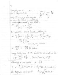
Question: Prove the validity of the kinematics equations by correlating the slope of
position time graphs to velocity graphs to acceleration graphs.
Please see graphs for calculations and discussion of reliability of figures
(uncertainty.)
Graph Set 1
Situation: Cart along a frictionless track, set level, no incline. Cart pushed to make it
travel fast. Sonic ranger and logger pro software created graphs.
We used the position graph to calculate the slope of a segment of the line. We used a
segment of the line where the slope appeared constant and positive (see graph 1, top
graph.)We used the following points:
Time (s) Position (m) Slope = change y /
change x
Y= position
X= time
Point 1 6.0 0.55 0.55-1.6/ Slope = 0.5
Point2 8.0 1.6 6.0-8.0 % error = 4%
The slope of the position graph should be equal to the velocity of the cart. The computer
calculated velocity at + 0 .64
We tested the formula, Velocity = (Xf-Xi)/(Tf-Ti), using the same points above
(substituting position points for X values.) Using this formula, we calculated velocity at
0.5 m/s.
We used our velocity chart to calculate the slope of a segment of the line. Since the
direction of the cart changed as it moved along the track, we again needed to find a line
segment in which the slope was constant. We used the following points:
Velocity (m/s) Time (s) Slope = change y
/change x
Y= velocity
X = time
Point 1 + 0.45 6.0 0.45-0.41/ Slope = -.02
Point 2 +.41 8.0 6.0-8.0 % error = 4%
The slope of the velocity graph should be equal to the acceleration of the cart. The

computer calculated acceleration at -0.05 m/s^2.
We tested the formula a=(Vf –Vi)/(Tf-Ti), using the same points above. Using this
formula , we calculated acceleration at -.02 m/s^2.
Graph Set 2
Situation: The situation for this set is the same as above with the exception that the cart
moves more slowly along the track.
Once again we used the position graph to calculate the slope of a segment of the line.
(See graph 2, top graph.) We used the following points:
Position (m) Time (s) Slope = change y
/ change x
Y = position
X = time
Point 1 1.66 4.00 1.66-1.31/ Slope = 0.24
Point 2 1.31 2.55 4.00-2.55 4.0 % error
The slope of the position graph should be equal to the velocity of the cart. The computer
calculated velocity at 0.28 m/s^2.
We tested the formula, Velocity = (Xf-Xi)/(Tf-Ti), using the same points above
(substituting position points for X values.) Using this formula, we calculated velocity at
0.24 m/s.
We used our velocity chart to calculate the slope of a segment of the line. We used the
following points:
Velocity (m/s) Time (s) Slope = change y
/ change x
Y = velocity
X = time
Point 1 0.30 2.0 0.30-0.20/ Slope =-0.05
Point2 0.20 4.0 2.0-4.0 4.0 % error
The slope of the velocity graph should be equal to the acceleration of the cart. The
computer calculated acceleration at -0.03 m/s^2.
We tested the formula a=(Vf –Vi)/(Tf-Ti), using the same points above. Using this
formula , we calculated acceleration at -.05m/s^2
Graph Set 3
Situation: Cart along a frictionless track, set on an incline of approximately 4 cm. Cart
was dropped at the height of the incline. Sonic ranger and logger pro software created
graphs.
We used the position graph to calculate the slope of a segment of the line. We used a
segment of the line where the slope appeared constant and positive (see graph 3, top
graph.)We used the following points:
Position (m) Time (s) Slope = change y
/ change x
Y = position
X = time
Point 1 1.1 1.0 1.65-1.1/ Slope = 0 .55
Point 2 1.65 2.0 2.0-1.0 4.0 % error
The slope of the position time graph should be equal to the velocity of the cart. The

computer calculated velocity at 0.44 m/s
We tested the formula, Velocity = (Xf-Xi)/(Tf-Ti), using the same points above
(substituting position points for X values.) Using this formula, we calculated velocity at
0.55 m/s.
We used our velocity chart to calculate the slope of a segment of the curved line. Because
the line was curved, we drew a line parallel to a segment of the curve and calculated the
slope. We used the following points:
Velocity (m/s) Time (s) Slope = change y
/ change x
Y = velocity
X = time
Point 1 0.44 6.5 0.44-.26 / Slope = 0.2
Point2 .26 5.6 6.5-5.6 4.0 % error
The slope of the velocity graph should be equal to the acceleration of the cart. The
computer calculated acceleration at .25 m/s^2
We tested the formula a=(Vf –Vi)/(Tf-Ti), using the same points above. Using this
formula , we calculated acceleration at 0.2 m/s^2.
Using the bottom graph of graph set three, we approximated the area of a rectangle of
space on the acceleration graph, or the area of the acceleration between acceleration
change, due to change in direction (see graph.) To find the length, we subtracted two
points on the time axis (X). To find the width, we subtracted two points on the
acceleration axis (Y).
Points
Difference
Length 0.357 – 0.103 0.254
Width 6.0 – 3.0 3.0
We multiplied the differences which would approximate the area of the rectangle. We
approximated the area of the rectangle at 0.762.
The distance of the same segment of line in the velocity graph spanned approximately
-0.5 m – 0.4 m, which is approximately -0.9 m in distance.
In conclusion, we used the slope of the position graph and correlated that to the velocity.
We used the slope of the velocity graph to find the acceleration.
We also were able to work in reverse.That is we were able to take two points on the
acceleration graph and drawing a rectangle down from them, we found the area of the
shape.Next we looked at the exact two points on the velocity graph, found the distance
between them and correlated this with the area of the formed rectangle on the
acceleration graph. We could have done the same thing using a rectangle's area on the
velocity graph and correlating it with the distance between the same points on the
distance graph.
This proves in both instances that when given one graph we can get information on the
others.