decision support system in city logistics - The Society for Modelling ...

More documents

Recommendations

Info

multiple objective metaheuristics in vehicle routing problem. (designed and verified on simulation data as add-in expanding functionality of TransCAD solver) In many real-world problems it is necessary to take into account many different and often conflicting objectives. In such problems there is no single optimal solution, but a set of many alternative solutions. At present multiple objective metaheuristics are a very active field of research. In this chapter author’s achievements in this field of research are summarized (for details see [1]). In our research an extended Capacitated Vehicle Routing Problem (CVRP) has been studied. This extension involves multiple objective optimization. Three independent objectives have been selected arbitrary: minimization of total traveling distance, traveling time and number of vehicles. Our multiple objective metaheuristics for CVRP have been based on Multiple Objective MetaHeuristic Library in C++ (MOMHLib++). MOMHLib++ is a library of C++ classes that implements a number of multiple objective metaheuristics. It has been developed by Jaszkiewicz (2001). In this library main multiple objectives metaheuristics are implemented in a consistent way, which allows easy adaptation of the methods to a given problem. As our main research interest lies in evolutionary computations, genetic algorithms have been selected from the MOMHLib++. These are (with working abbreviations used in the further part of this paper): 1. Strenght Pareto Evolutionary Approach (SPEA), 2. Nondominated Sorting Genetic Algorithm (NSGA), 3. Nondominated Sorting Genetic Algorithm II (NSGA II), 4. Controlled Nondominated Sorting Genetic Algorithm II (NSGA II C). Also hybrid genetic methods have been studied, where global optimization is hybridized with local optimization (local search method). These algorithms are: 1. Multiple Objective Genetic Local Search by Jaszkiewicz (MOGLS), 2. Multiple Objective Genetic Local Search by Ishibushi and Murata (IMMOGLS), 3. Pareto Memetic Algorithm (PMA). For the comparative purposes Multiple Objective Multiple Start Local Search (MOMSLS) method has been analyzed. During calculations two alternative mutation operation have been used: node exchange (NX) and arc exchange (AX). These two operations are adopted from the Traveling Salesperson Problem (TSP). In case of node exchange two points in the solution sequence are exchanged. In arc exchange operation the sequence between two points (including the second of the two selected points) is inverted. Each change in arcs is connected with changes in time and distances traveled by vehicles. Another operation is neighborhood search operation, which is necessary in local search optimization methods. For this purpose node exchange and arc exchange operators were used. But while in case of mutation the pairs of points are generated with randomness, in local search (where the neighborhood is searched in a systematical way) for each sensible pair the operation is performed. Experiments have been conducted in two phases. In first phase the single objective optimization has been carried out (minimization of the total distance). It is due to the fact that there are no benchmarks for the multiple objective CVRP. The single objective optimization was conducted to prove (with success) that: 1. Our genetic algorithm operators and local search method operators are well suited to the CVRP 2. Our software (which implements the CVRP and the operators) effectively works with MOMHLib++ In the second phase experiments on the multiple objective CVRP have been carried out. As a benchmark for the single objective CVRP optimization a number of well-known problem instances have been used. It includes instances form Augerat Set A (A-n44-k7, A-n54-k7, A-n80-k10), Augerat Set B (B-n31-k5, B-n41-k6, B-n57-k7, B-n63-k10, B-n78-k10) and Christofides and Eilon (E-n13-k4, E-n22-k4, E-n33-k4, E-n51-k5, E-n76-k10, E-n76-k14, E-n76-k7, E-n76-k8). Only few of those are presented in this paper. For each method and for each instance two kinds of optimizations have been carried out. In the first one AX operator has been used for mutation and local search, while in the other NX operator has been used. In case of genetic algorithms there is no significant difference in the results, so AX and NX operator are equally good for mutation. This has not come true in case of hybrid genetic algorithms and local search method, where AX and NX operators have been used for searching the neighborhood. In this case AX operator performs much better than NX. It is probably because less disturbances in solutions appear when AX is used, so this operator gives more chance to precisely search the current solution neighborhood. But more meaningful are differences in performance between algorithms. Best results have been obtained for the hybrid genetic algorithms (especially for MOGLS and PMA). Local search (MOMSLS) has performed well. The worst performance has been reached by the genetic algorithms (especially by SPEA and NSGA, see table 2). All four genetic algorithms use Pareto-ranking for assessing fitness for each chromosome. The poor performance of these genetic methods is due to the fact that Pareto ranking is not informative enough to carry out the optimization well.
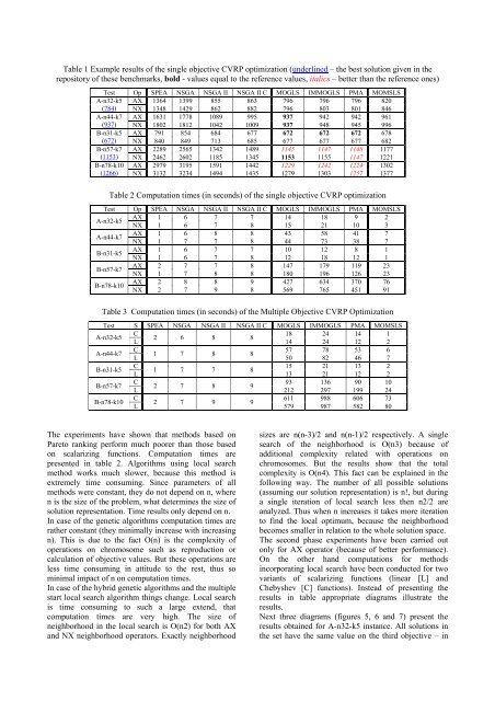
Table 1 Example results of the single objective CVRP optimization (underlined – the best solution given in the repository of these benchmarks, bold - values equal to the reference values, italics – better than the reference ones) Test Op SPEA NSGA NSGA II NSGA II C MOGLS IMMOGLS PMA MOMSLS A-n32-k5 AX 1364 1399 855 863 796 796 796 820 (784) NX 1348 1429 862 882 796 803 801 846 A-n44-k7 AX 1631 1778 1089 995 937 942 942 961 (937) NX 1802 1812 1042 1009 937 948 945 996 B-n31-k5 AX 791 854 684 677 672 672 672 678 (672) NX 840 849 713 685 677 677 677 682 B-n57-k7 AX 2289 2565 1342 1489 1145 1147 1148 1177 (1153) NX 2462 2602 1185 1345 1153 1155 1147 1221 B-n78-k10 AX 2979 3195 1591 1442 1229 1242 1224 1302 (1266) NX 3132 3234 1494 1435 1279 1303 1257 1377 Table 2 Computation times (in seconds) of the single objective CVRP optimization Test Op SPEA NSGA NSGA II NSGA II C MOGLS IMMOGLS PMA MOMSLS A-n32-k5 AX 1 6 7 7 14 18 9 2 NX 1 6 7 8 15 21 10 3 A-n44-k7 AX 1 6 8 8 43 58 41 7 NX 1 7 7 8 44 73 38 7 B-n31-k5 AX 1 6 7 7 10 12 8 1 NX 1 6 7 8 12 18 12 1 B-n57-k7 AX 2 7 7 8 147 179 119 23 NX 1 7 8 8 180 196 126 23 B-n78-k10 AX 2 8 8 9 427 634 370 76 NX 2 7 9 8 569 765 451 91 Table 3 Computation times (in seconds) of the Multiple Objective CVRP Optimization Test S SPEA NSGA NSGA II NSGA II C MOGLS IMMOGLS PMA MOMSLS A-n32-k5 C 18 24 14 1 2 6 8 8 L 14 24 12 2 A-n44-k7 C 57 78 53 6 1 7 8 8 L 50 82 46 7 B-n31-k5 C 15 21 13 2 1 7 7 8 L 13 21 12 2 B-n57-k7 C 93 136 90 10 2 7 8 9 L 212 297 199 24 B-n78-k10 C 611 988 606 73 2 7 9 9 L 579 987 582 80 The experiments have shown that methods based on Pareto ranking perform much poorer than those based on scalarizing functions. Computation times are presented in table 2. Algorithms using local search method works much slower, because this method is extremely time consuming. Since parameters of all methods were constant, they do not depend on n, where n is the size of the problem, what determines the size of solution representation. Time results only depend on n. In case of the genetic algorithms computation times are rather constant (they minimally increase with increasing n). This is due to the fact O(n) is the complexity of operations on chromosome such as reproduction or calculation of objective values. But these operations are less time consuming in attitude to the rest, thus so minimal impact of n on computation times. In case of the hybrid genetic algorithms and the multiple start local search algorithm things change. Local search is time consuming to such a large extend, that computation times are very high. The size of neighborhood in the local search is O(n2) for both AX and NX neighborhood operators. Exactly neighborhood sizes are n(n-3)/2 and n(n-1)/2 respectively. A single search of the neighborhood is O(n3) because of additional complexity related with operations on chromosomes. But the results show that the total complexity is O(n4). This fact can be explained in the following way. The number of all possible solutions (assuming our solution representation) is n!, but during a single iteration of local search less then n2/2 are analyzed. Thus when n increases it takes more iteration to find the local optimum, because the neighborhood becomes smaller in relation to the whole solution space. The second phase experiments have been carried out only for AX operator (because of better performance). On the other hand computations for methods incorporating local search have been conducted for two variants of scalarizing functions (linear [L] and Chebyshev [C] functions). Instead of presenting the results in table appropriate diagrams illustrate the results. Next three diagrams (figures 5, 6 and 7) present the results obtained for A-n32-k5 instance. All solutions in the set have the same value on the third objective – in
Page 1 and 2: DECISION SUPPORT SYSTEM IN CITY LOG
Page 3: this leads to an expert systems not

decision support system in city logistics - The Society for Modelling ...

Create successful ePaper yourself

Delete template?

Save as template?