Hydrography of the Russian River Estuary - Sonoma County Water ...
Hydrography of the Russian River Estuary - Sonoma County Water ...
Hydrography of the Russian River Estuary - Sonoma County Water ...

Create successful ePaper yourself
Turn your PDF publications into a flip-book with our unique Google optimized e-Paper software.
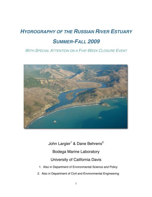
HYDROGRAPHY OF THE RUSSIAN RIVER ESTUARY<br />
SUMMER-FALL 2009<br />
WITH SPECIAL ATTENTION ON A FIVE-WEEK CLOSURE EVENT<br />
John Largier 1 & Dane Behrens 2<br />
Bodega Marine Laboratory<br />
University <strong>of</strong> California Davis<br />
1. Also in Department <strong>of</strong> Environmental Science and Policy<br />
2. Also in Department <strong>of</strong> Civil and Environmental Engineering<br />
1
Acknowledgements: This report was prepared for and funded by <strong>the</strong> <strong>Sonoma</strong><br />
<strong>County</strong> <strong>Water</strong> Agency. We thank Chris Delaney (SCWA), Matt Brennan (PWA),<br />
Fabian Bombardelli (UCD) and Jeff Church (SCWA) for valuable discussions. We<br />
thank Jeff Church at SCWA as well as Matt Robart, David Dann, Megan Sheridan,<br />
and o<strong>the</strong>r colleagues at BML/UCD for <strong>the</strong>ir assistance in <strong>the</strong> fieldwork – including<br />
summer REU student Aaron Tamminga. Warm thanks go to Elinor Twohy, whose<br />
hospitality was a critical help in <strong>the</strong> long days <strong>of</strong> fieldwork.<br />
2
Executive Summary<br />
Circulation, stratification and water properties were monitored during late summer 2009<br />
in <strong>the</strong> <strong>Russian</strong> <strong>River</strong> estuary– a dry year in which river flow was lower level than normal.<br />
Attention is directed at conditions in a month-long closure event in September-October.<br />
A dense lower layer <strong>of</strong> high-salinity water was trapped in <strong>the</strong> estuary when <strong>the</strong> mouth<br />
closed, with stability increasing over time as well as an expansion <strong>of</strong> stable stratification<br />
as saline waters intruded into <strong>the</strong> inner estuary. Within a week <strong>of</strong> strong stratification<br />
being established, <strong>the</strong> near-bottom waters became hypoxic. At mid-depth penetration <strong>of</strong><br />
light led to photosyn<strong>the</strong>sis and a stable layer in which oxygen levels were high during<br />
<strong>the</strong> day. At similar depths, <strong>the</strong>rmal radiation was also trapped and water temperatures<br />
were greatest. The thin surface layer was well mixed and in equilibrium with <strong>the</strong><br />
atmosphere in terms <strong>of</strong> both dissolved oxygen and temperature. Stratification and deepwater<br />
hypoxia persisted until tidal action returned with opening <strong>of</strong> <strong>the</strong> mouth in October.<br />
This report is preceded by a data report (Behrens & Largier 2010), in which all field data<br />
are plotted and details are provided on instrument deployments. In this report, core<br />
sections address (i) water budget and seepage analysis, (ii) tidal and diurnal currents,<br />
(iii) hydrographic structure – salinity, temperature, dissolved oxygen, (iv) stratification<br />
and water column stability, (v) salt and dissolved oxygen budgets.<br />
Central to this study and <strong>the</strong> value <strong>of</strong> <strong>the</strong> <strong>Russian</strong> <strong>River</strong> estuary as habitat for juvenile<br />
salmon is <strong>the</strong> strong stratification that develops due to trapping <strong>of</strong> a salt layer in <strong>the</strong><br />
estuary when <strong>the</strong> mouth closes. The salt-stratified closed estuary is non-tidal and a<br />
wind-driven diurnal seiche takes on particular importance in <strong>the</strong> horizontal redistribution<br />
<strong>of</strong> salt as well as in raising <strong>the</strong> possibility <strong>of</strong> vertical mixing and eventual breakdown <strong>of</strong><br />
<strong>the</strong> stratification. Breakdown <strong>of</strong> stratification appears essential for re-oxygenating <strong>the</strong><br />
hypoxic bottom waters and reducing mid-depth temperatures. A significant apparent<br />
loss <strong>of</strong> estuary water through <strong>the</strong> sand barrier (~60cfs) is important in flushing <strong>the</strong><br />
surface layer (residence time order 10 days), but it plays only a minor role in reducing<br />
<strong>the</strong> salinity <strong>of</strong> <strong>the</strong> lower layer within 1-2 km <strong>of</strong> <strong>the</strong> barrier beach.<br />
The most significant advances in future understanding in support <strong>of</strong> improved<br />
management <strong>of</strong> <strong>the</strong> estuary are likely to come from (i) linking water property<br />
distributions to salmon habitat value and extent, (ii) assessment <strong>of</strong> <strong>the</strong> extent <strong>of</strong> hypoxia<br />
immediately following breaching after a long closure, (iii) assessment <strong>of</strong> turbulence,<br />
vertical mixing and <strong>the</strong> potential for breakdown <strong>of</strong> stratification, (iv) a fuller quantification<br />
and understanding <strong>of</strong> <strong>the</strong> diurnal wind-driven seiche, (v) a fuller quantification and<br />
understanding <strong>of</strong> seepage losses through <strong>the</strong> sand barrier, and (vi) a fuller quantification<br />
and understanding <strong>of</strong> berm overflows and wave overwash.<br />
3
This page intentionally blank.<br />
4
Table <strong>of</strong> Contents<br />
1. Introduction ............................................................................................ 7<br />
2. Field Data............................................................................................. 8<br />
2.1 – Time-series <strong>of</strong> water level elevations ..............................................................9<br />
2.2 – Boat-based CTD surveys.................................................................................10<br />
2.3 – Time-series <strong>of</strong> vertical pr<strong>of</strong>iles <strong>of</strong> currents...................................................10<br />
2.4 – Time-series <strong>of</strong> water temperature and salinity .............................................10<br />
2.5 – <strong>Estuary</strong> bathymetry..........................................................................................11<br />
2.6 – Meteorological data .........................................................................................12<br />
2.7 – Wave measurements .......................................................................................12<br />
2.8 – <strong>River</strong> flow measurements ...............................................................................12<br />
3. Data Analysis ...................................................................................... 13<br />
3.1 – <strong>Water</strong> budget & Seepage analysis .................................................................13<br />
3.1.1 – Historical closure events..............................................................................14<br />
3.1.2 – Estimation <strong>of</strong> seepage rate ..........................................................................15<br />
3.1.3 – Relation between seepage loss and water level..........................................19<br />
3.2 – Tidal and diurnal currents ...............................................................................23<br />
3.2.1 – Current velocities at Paddyʼs Rock ..............................................................24<br />
3.2.2 – Current velocities at Heron Rookery ............................................................27<br />
3.2.3 – Diurnal wind-driven seiche...........................................................................30<br />
3.3 – Hydrographic structure ...................................................................................34<br />
3.3.1 – Spatial distribution <strong>of</strong> salinity .......................................................................35<br />
3.3.2 – Salt intrusion into inner estuary ...................................................................37<br />
3.3.3 – Spatial distribution <strong>of</strong> temperature ...............................................................38<br />
3.3.4 – Spatial distribution <strong>of</strong> dissolved oxygen.......................................................41<br />
3.4 – Stratification and water-column stability.......................................................45<br />
3.4.1 – Richardson Number – assessing stability as a function <strong>of</strong> depth ................46<br />
3.4.2 – Assessing water column stability – <strong>the</strong> potential energy anomaly...............50<br />
3.5 – Salt and oxygen mass budgets ......................................................................55<br />
3.5.1 – Salt budget for estuary.................................................................................55<br />
3.5.2 – Preliminary dissolved oxygen budget for estuary ........................................60<br />
3.5.3 – Sources <strong>of</strong> error in budgets..........................................................................63<br />
4. Discussion......................................................................................... 67<br />
5. Literature Reviewed ......................................................................... 70<br />
5
Acronyms & Terminology<br />
ADCP<br />
anoxic<br />
barotropic<br />
baroclinic<br />
BML<br />
BOD<br />
BOON<br />
CDIP<br />
CTD<br />
DO<br />
DWR<br />
halocline<br />
hypoxic<br />
acoustic doppler current pr<strong>of</strong>iler<br />
zero dissolved oxygen<br />
pressure gradient due to sloping water level is uniform with depth<br />
pressure gradient due to gradient in density increases with depth<br />
Bodega Marine Laboratory, University <strong>of</strong> California Davis<br />
biochemical oxygen demand<br />
Bodega Ocean Observing Node (http://www.bml.ucdavis.edu/boon/)<br />
Coastal Data Information Program (http://cdip.ucsd.edu/)<br />
conductivity-temperature-depth pr<strong>of</strong>iling instrument<br />
dissolved oxygen<br />
California Department <strong>of</strong> <strong>Water</strong> Resources<br />
level at which salinity changes suddenly with depth<br />
very low level <strong>of</strong> dissolved oxygen (typically below 2mg/l)<br />
hypsometric curve that shows plan area <strong>of</strong> estuary at different elevations (when<br />
curve integrated, curve gives estuary volume below that elevation)<br />
iso<strong>the</strong>rmal<br />
isopycnal<br />
NDBC<br />
NMFS<br />
PAR<br />
ppt<br />
psu<br />
PWA<br />
pycnocline<br />
SBE<br />
SCWA<br />
seiche<br />
no spatial difference in temperature<br />
no spatial difference in density; or line <strong>of</strong> equal density<br />
National Data Buoy Center (http://www.ndbc.noaa.gov/)<br />
National Marine Fisheries Service (http://www.nmfs.noaa.gov/)<br />
photosyn<strong>the</strong>tically active radiation<br />
parts per thousand (by mass)<br />
practical salinity units<br />
Philip Williams & Associates (http://www.pwa-ltd.com/)<br />
level at which density changes suddenly<br />
SeaBird Electronics (http://www.seabird.com/)<br />
<strong>Sonoma</strong> <strong>County</strong> <strong>Water</strong> Agency (http://www.scwa.ca.gov/)<br />
rhythmic swash <strong>of</strong> water in a basin, from one end to <strong>the</strong> o<strong>the</strong>r, and back<br />
<strong>the</strong>rmocline level at which temperature changes suddenly<br />
6
1. Introduction<br />
The <strong>Russian</strong> <strong>River</strong> Biological Opinion written by <strong>the</strong> National Marine Fisheries Service<br />
(NMFS 2008) requires <strong>the</strong> <strong>Sonoma</strong> <strong>County</strong> <strong>Water</strong> Agency (SCWA) to manage <strong>the</strong><br />
<strong>Russian</strong> <strong>River</strong> estuary in such a way as to maintain a closed mouth following natural<br />
closure during <strong>the</strong> summer management period <strong>of</strong> 15 May through 15 October. It is<br />
expected that this closed lagoon state was typical in late summer and fall prior to human<br />
perturbations <strong>of</strong> <strong>the</strong> system and that this closed lagoon state will provide improved<br />
habitat for <strong>the</strong> rearing <strong>of</strong> juvenile steelhead in <strong>the</strong> estuary (and possibly also coho).<br />
However, long-duration closures <strong>of</strong> <strong>the</strong> <strong>Russian</strong> <strong>River</strong> estuary have not been observed<br />
recently and it is unclear how stratification and water residence will play out in terms <strong>of</strong><br />
<strong>the</strong> distribution <strong>of</strong> water properties (specifically salinity, temperature, velocity, and<br />
dissolved oxygen). <strong>Water</strong> properties are key determinants <strong>of</strong> juvenile steelhead habitat,<br />
and <strong>the</strong>y are important in <strong>the</strong>ir relation to water quality conditions conducive to<br />
ecosystem health and human “beneficial uses”.<br />
Bodega Marine Laboratory (BML) at <strong>the</strong> University <strong>of</strong> California Davis was contracted by<br />
<strong>the</strong> SCWA to conduct a study <strong>of</strong> <strong>the</strong> estuary that provides a view <strong>of</strong> circulation,<br />
stratification, salinity, and residence during <strong>the</strong> summer and fall <strong>of</strong> 2009. The aim was to<br />
provide SCWA with a basis for designing a more complete hydrological analysis by<br />
identifying phenomena and processes that are critical to future management <strong>of</strong> <strong>the</strong><br />
estuary and <strong>the</strong> multiple human and ecosystem uses <strong>of</strong> this environment. Data were<br />
collected as a basis for (i) assessment <strong>of</strong> <strong>the</strong> hydrological condition <strong>of</strong> <strong>the</strong> estuary during<br />
<strong>the</strong> 2009 dry season, (ii) future analyses that will provide understanding <strong>of</strong> how river<br />
flow and mouth state control estuary hydrology and through that water-column habitat in<br />
<strong>the</strong> estuary, and (iii) validation and inputs for future numerical modeling <strong>of</strong> <strong>the</strong> estuary.<br />
The <strong>Russian</strong> <strong>River</strong> estuary is a bar-built, drowned-river-valley estuary. Although this<br />
type <strong>of</strong> estuary is common – indeed typical – in central and nor<strong>the</strong>rn California, <strong>the</strong><br />
characteristic hydrological patterns and underlying hydrodynamic processes are not well<br />
documented nor understood. In this study, it was necessary to obtain primary field data<br />
and to conduct data analyses in order to obtain a preliminary understanding <strong>of</strong> this<br />
system and thus to allow discussion <strong>of</strong> possible future conditions.<br />
This report is a summary <strong>of</strong> results from <strong>the</strong> field program in <strong>the</strong> <strong>Russian</strong> <strong>River</strong> estuary<br />
during <strong>the</strong> summer and fall <strong>of</strong> 2009, during which river flows were lower than normal.<br />
This report is preceded by a data report (Behrens & Largier 2010), in which all field data<br />
are described and graphically presented.<br />
7
2. Field Data<br />
The study area extended from <strong>the</strong> mouth <strong>of</strong> <strong>the</strong> <strong>Russian</strong> <strong>River</strong> estuary to Austin Creek.<br />
Fieldwork consisted <strong>of</strong> four components, described below (Figure 2.1):<br />
(1) Time-series <strong>of</strong> pressure/temperature measurements at 4 locations, for monitoring<br />
water surface elevation.<br />
(2) Vertical pr<strong>of</strong>iles <strong>of</strong> conductivity-temperature-depth (CTD) at fixed stations along <strong>the</strong><br />
axis <strong>of</strong> estuary.<br />
(3) Time-series <strong>of</strong> vertical pr<strong>of</strong>iles <strong>of</strong> currents – acoustic doppler current pr<strong>of</strong>iler (ADCP).<br />
(4) Time-series <strong>of</strong> near-bottom salinity/temperature measurements at 3 locations.<br />
These data are described in detail and all data are plotted in <strong>the</strong> companion data report<br />
(Behrens & Largier 2010). These data are combined with sonde data from SCWA and<br />
with data on waves, river flow, wind and bathymetry obtained from o<strong>the</strong>r sources (see<br />
below) to provide a description <strong>of</strong> hydrographic conditions and an understanding <strong>of</strong><br />
hydrodynamic controls in <strong>the</strong> <strong>Russian</strong> <strong>River</strong> estuary during late summer and fall 2009.<br />
Figure 2.1. Measurement locations: 1 - Mouth, 2 - Paddy's Rock, 3 - Bridgehaven,<br />
4 - Willow Creek, 5 - Sheephouse Creek, 6- Osprey Rookery, 7 - Heron Rookery,<br />
8 - Freezeout Island, 9 - Freezeout Creek and 10 - Moscow Bridge.<br />
8
The study was conducted from June through December 2009. The estuary mouth<br />
remained open following a brief closure period in late June and tidal fluctuations in <strong>the</strong><br />
estuary reflected spring-neap cycles and <strong>the</strong> degree <strong>of</strong> tidal constriction at <strong>the</strong> mouth.<br />
An extended mouth closure event started on 7 September, following several days <strong>of</strong><br />
muted tides (Figure 2.2). The mouth remained closed until 6 October. It remained open<br />
for about a week before closing again in mid-October. The September-October event<br />
provided an opportunity to study <strong>the</strong> conditions during a prolonged closure event at high<br />
temporal resolution.<br />
Figure 2.2 <strong>Water</strong> level record during study period, providing a study timeline and<br />
indicating periods <strong>of</strong> ADCP deployment (horizontal grey bars) and times that CTD<br />
pr<strong>of</strong>iles were taken (vertical dashed lines).<br />
2.1 – Time-series <strong>of</strong> water level elevations<br />
Four HOBO water level loggers were deployed in August, at locations shown in Figure<br />
2.1. The loggers record temperature and pressure at two-minute intervals. Atmospheric<br />
pressure (measured at BML) was subtracted from <strong>the</strong> measured pressure to obtain<br />
9
gage pressure (i.e., pressure due to <strong>the</strong> weight <strong>of</strong> <strong>the</strong> overlying water). Gage pressure<br />
and temperature were used in conjunction with surface salinity obtained from SCWA<br />
sondes to calculate water density from <strong>the</strong> UNESCO (1981) Equation <strong>of</strong> State. Using<br />
this density, <strong>the</strong> height <strong>of</strong> water above <strong>the</strong> gage was calculated by assuming hydrostatic<br />
conditions. All four gages were referenced to <strong>the</strong> NGVD datum by comparing data with<br />
data from <strong>the</strong> SCWA gage at Jenner, which has been surveyed in to NGVD. By<br />
identifying a time during inlet closure (i.e., no tide) when river flow and wind are minimal,<br />
one can assume that <strong>the</strong> water surface is horizontal throughout <strong>the</strong> estuary and make<br />
direct comparisons between gages. Given <strong>the</strong> uncertainty involved in this method, <strong>the</strong><br />
elevations estimated for <strong>the</strong> loggers are assumed to be accurate to within ±5cm,<br />
however, when considering changes in slope, this error cancels out and gages will have<br />
an accuracy as specified (i.e.,
attached to each ADCP, and a third one was located in a shallow channel adjacent to<br />
Freezeout Island, between <strong>the</strong> Heron Rookery and Freezeout Creek pr<strong>of</strong>iling stations. In<br />
addition, several YSI 6600 datasondes had been deployed by SCWA in May, recording<br />
data on temperature, salinity, pH, pressure and dissolved oxygen at near-surface, middepth<br />
and near-bottom depths (depending on location). At Paddy's Rock and Heron<br />
Rookery, <strong>the</strong> near-surface SCWA sondes were combined with near-bottom MicroCats to<br />
obtain top-bottom density differences used in stability calculations (Section 4.3). Middepth<br />
sondes at Sheephouse Creek, Heron Rookery and Freezeout Creek (as well as<br />
near-bottom sondes at Heron Rookery and Freezeout) were also used to monitor<br />
salinity intrusion during tidal conditions. The MicroCat deployed at Freezeout Island<br />
provided additional detail on intrusions <strong>of</strong> saline waters at depth.<br />
Contour plots <strong>of</strong> <strong>the</strong> longitudinal distribution <strong>of</strong> temperature, salinity or dissolved oxygen<br />
is obtained by interpolating between pr<strong>of</strong>ile locations using a cubic-spline interpolation<br />
scheme in MATLAB. The longitudinal depth pr<strong>of</strong>ile is derived from <strong>the</strong> bathymetry. The<br />
entire set is presented in <strong>the</strong> data report, and examples are presented in Chapter 3. In<br />
this analysis, it is assumed that lateral structure is homogeneous (or nearly so), so that<br />
<strong>the</strong> 2-dimensional along-and-vertical contour plot is representative <strong>of</strong> <strong>the</strong> whole estuary.<br />
Lateral structure will be investigated in future work, specifically exploring differences<br />
between <strong>the</strong> channel center and shallow littoral waters.<br />
2.5 – <strong>Estuary</strong> bathymetry<br />
The high-resolution 2009 survey <strong>of</strong> estuary bathymetry (EDS, 2009) was used for this<br />
analysis. The continuous surface generated by PWA, using <strong>the</strong> triangular interpolated<br />
network (TIN) approach, was sampled to produce a 10m x 10m raster file. This grid was<br />
used to obtain a longitudinal thalweg pr<strong>of</strong>ile for <strong>the</strong> estuary, and in calculation <strong>of</strong> stagestorage<br />
relations for <strong>the</strong> entire estuary and for individual reaches. These stage-storage<br />
relations are used in seepage calculations (Section 3.1) and in salt and dissolved<br />
oxygen budgets (Sections 3.7 and 3.8).<br />
11
2.6 – Meteorological data<br />
Meteorological data on wind speed, air temperature, barometric pressure and relative<br />
humidity were obtained from sensors at Bodega Marine Laboratory, approximately 12<br />
miles south <strong>of</strong> <strong>the</strong> mouth <strong>of</strong> <strong>the</strong> <strong>Russian</strong> <strong>River</strong>. While wind speed may vary between<br />
BML and <strong>the</strong> mouth, <strong>the</strong> wind at <strong>the</strong> two locations is expected to be well correlated, with<br />
strong wind or calm conditions being experienced concurrently in this region (including<br />
<strong>the</strong> estuary closest to <strong>the</strong> mouth). More importantly, wind speed and direction varies<br />
along <strong>the</strong> estuary, with airflow generally following <strong>the</strong> valley orientation, but with some<br />
locations being sheltered by <strong>the</strong> adjacent hills. As such, BML wind data are used as an<br />
index <strong>of</strong> <strong>the</strong> importance <strong>of</strong> wind forcing. In contrast, it is expected that air temperature,<br />
barometric pressure and relative humidity vary little between BML and <strong>the</strong> <strong>Russian</strong><br />
<strong>River</strong> mouth.<br />
2.7 – Wave measurements<br />
Deep-water wave height data were obtained from <strong>the</strong> CDIP Pt. Reyes Buoy (Buoy #29).<br />
These data were converted to estimates <strong>of</strong> wave height at <strong>the</strong> 10m isobath <strong>of</strong>fshore <strong>of</strong><br />
<strong>the</strong> <strong>Russian</strong> <strong>River</strong> mouth using a transformation matrix provided by CDIP. The matrix for<br />
converting <strong>of</strong>fshore wave heights to nearshore values accounts for wave refraction and<br />
shoaling, and is described fur<strong>the</strong>r in Battalio et al (2006) and Behrens et al (2009).<br />
2.8 – <strong>River</strong> flow measurements<br />
<strong>River</strong> flow data are available for <strong>the</strong> <strong>Russian</strong> <strong>River</strong> at Johnsons Beach at Guerneville<br />
(USGS Site 11467002) and also fur<strong>the</strong>r upstream at Hacienda Bridge (USGS Site<br />
11467000). As <strong>the</strong>re are many opportunities for inflow or extraction between <strong>the</strong>se sites<br />
and <strong>the</strong> head <strong>of</strong> <strong>the</strong> estuary, SCWA provided additional flow measurements at Vacation<br />
Beach, which is much nearer <strong>the</strong> upstream boundary <strong>of</strong> <strong>the</strong> estuary. Flow was<br />
measured using an impeller-based device at width intervals across <strong>the</strong> channel. Flow<br />
measurements were compared with water level measurements to provide a flow-stage<br />
relationship. Then a continuous water-level record was used and data interpreted as<br />
flow rates, based on <strong>the</strong> above relationship. These flow-rate estimates were used to<br />
determine <strong>the</strong> contribution <strong>of</strong> river flow to <strong>the</strong> estuary volume as part <strong>of</strong> <strong>the</strong> water budget<br />
model (Section 3.1).<br />
12
3. Data Analysis<br />
The results from several analyses are reported in this section. A full representation <strong>of</strong><br />
<strong>the</strong> data is available in <strong>the</strong> companion data report (Behrens & Largier 2010). Here we<br />
address specific issues:<br />
(1) An estimate is obtained for water lost as seepage through <strong>the</strong> sand barrier at <strong>the</strong><br />
mouth by calculating a budget <strong>of</strong> water flow into and out <strong>of</strong> <strong>the</strong> estuary.<br />
(2) Tidal flows and diurnal wind-driven seiche flows are quantified through an analysis <strong>of</strong><br />
data on current velocities and water level fluctuations.<br />
(3) The spatial distribution <strong>of</strong> salinity is described, specifically addressing intrusion <strong>of</strong><br />
salinity upstream during open and closed periods.<br />
(4) The spatial distribution <strong>of</strong> water temperature is described and changes during <strong>the</strong><br />
long closure event are outlined.<br />
(5) The spatial distribution <strong>of</strong> dissolved oxygen is described, identifying locations and<br />
times when anoxic or hypoxic conditions are found at depth.<br />
(6) Stratification is quantified and analysis <strong>of</strong> <strong>the</strong> stability <strong>of</strong> this stratification provides a<br />
measure <strong>of</strong> <strong>the</strong> likelihood <strong>of</strong> mixing between deep saline water and surface freshwater.<br />
(7) A salt budget is calculated for <strong>the</strong> long closure event.<br />
(8) An oxygen budget is calculated for <strong>the</strong> lower layer.<br />
3.1 – <strong>Water</strong> budget & Seepage analysis<br />
At <strong>the</strong> heart <strong>of</strong> <strong>the</strong> NMFS-proposed management protocol for <strong>the</strong> <strong>Russian</strong> <strong>River</strong> estuary<br />
is <strong>the</strong> concept that water will escape from a closed estuary by seeping through <strong>the</strong> sand<br />
barrier that separates it from <strong>the</strong> ocean. This will happen due to <strong>the</strong> rise <strong>of</strong> <strong>the</strong> elevation<br />
<strong>of</strong> <strong>the</strong> estuary water level above that in <strong>the</strong> ocean (i.e., a scenario typically described as<br />
a “perched lagoon”). This “seepage loss” may be accompanied by a flow <strong>of</strong> water over<br />
<strong>the</strong> sand barrier (which is also known as <strong>the</strong> “berm”, referring to its wave-built origin).<br />
Such an “overflow” at <strong>the</strong> mouth <strong>of</strong> <strong>the</strong> <strong>Russian</strong> <strong>River</strong> is not common in recent times<br />
(PWA 2009), and <strong>the</strong> future flow rate is expected to be much lower than typical river<br />
inflow rates in <strong>the</strong> past, even in dry years, so that a significant seepage loss is required<br />
to maintain a steady water level in <strong>the</strong> estuary. Both overflow and expulsion <strong>of</strong> deeper<br />
saline waters through <strong>the</strong> sand barrier occur in comparable smaller estuaries along <strong>the</strong><br />
coast <strong>of</strong> California, as noted in NMFS (2008).<br />
13
3.1.1 – Historical closure events<br />
In <strong>the</strong> past, closure events have <strong>of</strong>ten lasted several weeks without breaching, despite<br />
<strong>the</strong> lack <strong>of</strong> accommodation space for cumulative inflow. Without significant loss <strong>of</strong> water<br />
from <strong>the</strong> estuary, closures <strong>of</strong> <strong>the</strong> <strong>Russian</strong> <strong>River</strong> mouth would be short-lived: given river<br />
inflows on <strong>the</strong> order <strong>of</strong> 100 cfs, <strong>the</strong> estuary water level would reach stages in excess <strong>of</strong><br />
7ft NGVD29 within 1-2 weeks without some form <strong>of</strong> water loss. Extensive records <strong>of</strong><br />
inflows near Guerneville and closure duration at <strong>the</strong> mouth indicate that several closures<br />
have endured much longer. This suggests that <strong>the</strong>re is a significant export <strong>of</strong> water from<br />
<strong>the</strong> estuary that <strong>of</strong>fsets inflow during closure events.<br />
Figure 3.1. Closure durations and median flows observed by Rice (1974) and Behrens<br />
et al. (2009).<br />
In Figure 3.1, closure duration is compared with median inflow for about 150 events<br />
spanning five decades. A DWR gage operated between 1939 and 1955 was used by<br />
Rice (1974) to infer closure events, while closure events after 1973 were observed<br />
directly by Elinor Twohy, a resident <strong>of</strong> Jenner (Behrens et al. 2009). The earlier record<br />
does not reflect all closure events, as <strong>the</strong> gage occasionally malfunctioned. One can<br />
see that closure durations tend to be much shorter during <strong>the</strong> more recent period, due to<br />
<strong>the</strong> D1610 decision in 1986 that required minimum summer flows combined with <strong>the</strong><br />
14
existing SCWA-management protocol that requires an artificial breach when Jenner<br />
stage exceeds 7ft NGVD29. Although local residents breached <strong>the</strong> barrier at times<br />
during <strong>the</strong> earlier period (Rice, 1974), <strong>the</strong>y were less frequent – consistent with <strong>the</strong><br />
observation <strong>of</strong> closures lasting much more than two weeks.<br />
An interesting characteristic <strong>of</strong> <strong>the</strong>se data is that for many <strong>of</strong> <strong>the</strong> closure events lasting<br />
for more than 20 days, <strong>the</strong> median flow was in excess <strong>of</strong> 70cfs (indeed many had<br />
inflows on <strong>the</strong> order <strong>of</strong> 100cfs or more). These closures could only persist if <strong>the</strong>re were<br />
a concomitant loss <strong>of</strong> water from <strong>the</strong> estuary basin <strong>of</strong> <strong>the</strong> same order <strong>of</strong> magnitude. We<br />
use this principle in <strong>the</strong> next section to obtain an estimate <strong>of</strong> seepage rates.<br />
3.1.2 – Estimation <strong>of</strong> seepage rate<br />
An estimation <strong>of</strong> water loss from <strong>the</strong> estuary basin can be obtained by comparing<br />
inflows and outflows with changes in <strong>the</strong> volume <strong>of</strong> water in <strong>the</strong> basin, i.e., a water<br />
budget for <strong>the</strong> estuary. Equation (1) expresses this balance, explicitly listing all <strong>of</strong> <strong>the</strong><br />
terms, which are illustrated in Figure 3.2. This budget treats <strong>the</strong> estuary as a box with<br />
well-defined lower and upper boundaries – <strong>the</strong> mouth and Vacation Beach, respectively.<br />
Measured bathymetry (EDS, 2009) was used to characterize <strong>the</strong> estuary shape and<br />
volume for different water levels (hypsometric curve). Budgets are constructed for all<br />
days when <strong>the</strong> mouth was closed during <strong>the</strong> ten-year period from 1999 to 2009.<br />
Figure 3.2. <strong>Estuary</strong> schematic detailing processes relevant to changes in volume during<br />
closure (“personal wells” is synonymous with “domestic wells”).<br />
15
Equation 1 shows that changes in <strong>the</strong> volume <strong>of</strong> water in <strong>the</strong> estuary must be explained<br />
by inputs (river inflow + wave overwash + precipitation on surface) minus outputs<br />
(evaporation across surface + seepage through <strong>the</strong> sand barrier + seepage into aquifers<br />
+ extraction).<br />
(dV/dt) estuary = Q river + Q overwash + P – E – (Q seep + Q aquifer ) – Q extract [Eq. 1]<br />
where V represents <strong>the</strong> estuary volume, t represents time, P and E are precipitation and<br />
evaporation rates, and Q represents a flow rate. Using a 24-hour time step, <strong>the</strong> rate <strong>of</strong><br />
water added or subtracted from <strong>the</strong> estuary is estimated for each term, as described<br />
below.<br />
1. Change in estuary volume: This was calculated from changes in water level, using<br />
<strong>the</strong> hypsometric curve calculated from EDS bathymetric data.<br />
2. <strong>River</strong> inflow: This was quantified through a stage-flow relationship obtained by<br />
SCWA at Vacation Beach, to account for inputs and extraction from <strong>the</strong> river below<br />
<strong>the</strong> USGS Hacienda Bridge gage. This inflow assumes negligible surface inflow from<br />
Austin Creek and o<strong>the</strong>r smaller creeks that are below Vacation Beach. For higher<br />
flow rates that exceeded <strong>the</strong> range <strong>of</strong> data in this relationship, flows from <strong>the</strong><br />
Hacienda Gage were used.<br />
3. Wave overwash: This occurs rarely, as well-defined events. Days on which<br />
overwash is known to occur are excluded from this analysis, and it is assumed that<br />
overwash is negligible for o<strong>the</strong>r days.<br />
4. Precipitation: Given that longer closures occur during <strong>the</strong> summer and fall seasons<br />
when rainfall is typically absent, precipitation is assumed to be zero. Rainfall records<br />
were used to confirm <strong>the</strong> absence <strong>of</strong> rain during <strong>the</strong> events analyzed here.<br />
5. Evaporation: This was calculated using <strong>the</strong> method <strong>of</strong> Linacre (1992), which does<br />
not require continuous water temperature data. It is assumed to provide sufficient<br />
accuracy given that total evaporation losses were between 0 and 5cfs, one to two<br />
orders <strong>of</strong> magnitude less than river inflows (typically 70-300cfs) and calculated<br />
seepage losses (30-100cfs).<br />
6. Seepage loss: This term refers to an outflow from <strong>the</strong> perched estuary through <strong>the</strong><br />
sand barrier at <strong>the</strong> mouth. It is combined with <strong>the</strong> next term into a single unknown<br />
loss term.<br />
16
7. Loss to aquifers: This term quantifies groundwater-surface water interactions and it<br />
can be positive (i.e., flux from estuary to aquifer) or negative (i.e., flux from aquifer to<br />
estuary). It is combined with <strong>the</strong> previous term into a single unknown loss term.<br />
8. Extraction: Withdrawal <strong>of</strong> water is only via domestic wells within <strong>the</strong> model domain.<br />
This can be shown to be a negligible flow rate, considering typical rates <strong>of</strong> domestic<br />
water use.<br />
Re-arranging Equation 1, one gets a simple expression for <strong>the</strong> combined unknown loss<br />
term Q loss = Q seep + Q aquifer :<br />
Q loss = Q river - E - (dV/dt) estuary [Eq. 2]<br />
There are no data on <strong>the</strong> flux <strong>of</strong> estuarine waters to local aquifers Q aquifer and thus this<br />
term is retained in <strong>the</strong> combined loss term, but it is expected that Q loss is primarily due to<br />
<strong>the</strong> seepage term and <strong>the</strong>se terms are used interchangeably in <strong>the</strong> following discussion.<br />
Unknown bathymetry<br />
High-resolution bathymetry data are available as far upstream as <strong>the</strong> confluence with<br />
Austin Creek, and some distance into Jenner Gulch, Willow Creek and Freezeout<br />
Creek, but bathymetry is poorly known upstream <strong>of</strong> Austin Creek. In closure periods,<br />
water levels can rise as far upstream as Vacation Beach, about 10 km above Austin<br />
Creek.<br />
Figure 3.3. Comparison <strong>of</strong> estimates for estuary surface upstream <strong>of</strong> Austin Creek<br />
17
Bathymetry in this reach was estimated from channel pr<strong>of</strong>iles measured by Goodwin &<br />
Cuffe (1994). The relative importance <strong>of</strong> backing up water upstream <strong>of</strong> Austin Creek<br />
was assessed by corrections to <strong>the</strong> hypsometric curve, expressing surface area in this<br />
“upper” reach as a fraction <strong>of</strong> total area (Figure 3.3). The best fit to Goodwin and Cuffe's<br />
data is shown as well as 25% errors as upper- and lower-bound estimates, which are<br />
expected to bound <strong>the</strong> unknown real values.<br />
As shown in Figure 3.4, a 25% uncertainty in <strong>the</strong> volume upstream <strong>of</strong> Austin Creek<br />
introduces a small error in quantifying <strong>the</strong> total estuary volume (error is order 1% at 8ft<br />
NGVD). This is because significant amounts <strong>of</strong> water do not backup into this region until<br />
<strong>the</strong> estuary stage is high. Even at 8 ft NGVD this uncertainty accounts for no more than<br />
a 2cfs error in estimates <strong>of</strong> loss.<br />
Figure 3.4. <strong>Estuary</strong> stage-volume relation comparing methods <strong>of</strong> estimating upstream<br />
surface area<br />
Wave overwash<br />
Data recorded during <strong>the</strong> September 2009 closure event and o<strong>the</strong>r historical events<br />
have shown a sudden increase in estuary water level during periods <strong>of</strong> high waves. For<br />
example, between September 12 and 14 <strong>the</strong> water level in <strong>the</strong> estuary rose 0.4m<br />
(~1.5ft) during a prolonged period with nearshore wave heights exceeding 4m (see<br />
18
Figure 3.7). A concurrent drop in estuary temperature and increase in <strong>the</strong> mass <strong>of</strong> salt in<br />
<strong>the</strong> estuary salt mass (see Figure 3.39) indicate that wave overwash was indeed <strong>the</strong><br />
cause <strong>of</strong> <strong>the</strong> water-level change. As wave-overwash volumes are difficult to estimate<br />
without direct data, or data on berm morphology (e.g. height, width), <strong>the</strong>se days were<br />
excluded from water budget calculations. Days were excluded if wave heights exceeded<br />
1.2m (~4ft) or if wave heights exceeded <strong>the</strong> difference between estuary and ocean<br />
levels by more than 0.3m (~1ft).<br />
3.1.3 – Relation between seepage loss and water level<br />
The loss <strong>of</strong> water owing to seepage through <strong>the</strong> sand barrier at <strong>the</strong> mouth is driven by<br />
<strong>the</strong> pressure difference across <strong>the</strong> barrier due to <strong>the</strong> difference in water level between<br />
estuary and ocean. The rate <strong>of</strong> flow Q seep is expressed by Darcyʼs Law:<br />
Q seep = K.A.dh/dL [Eq. 3]<br />
where K is <strong>the</strong> hydraulic conductivity (related to permeability <strong>of</strong> <strong>the</strong> barrier), A is <strong>the</strong><br />
cross-sectional area <strong>of</strong> <strong>the</strong> flow through <strong>the</strong> barrier, and dh/dL is <strong>the</strong> hydraulic gradient<br />
(hydraulic head divided by length <strong>of</strong> flow path). Thus, as <strong>the</strong> estuary water level rises<br />
one expects <strong>the</strong> seepage rate to increase (given that ocean water level changes little at<br />
time scales longer than tidal).<br />
Here <strong>the</strong> loss term from Equation 2 is plotted against <strong>the</strong> difference between Jennergage<br />
estuary water level and 25-hour averages <strong>of</strong> <strong>the</strong> sea level at <strong>the</strong> Pt. Reyes tide<br />
gage (Figure 3.5). The difference Δh produces a better fit with flow loss estimates than<br />
<strong>the</strong> Jenner gage level alone, because <strong>the</strong> sea level is not constant but varies in<br />
response to winds and waves (Largier et al 1993; O'Callahan et al 2007), which have a<br />
different local effect on <strong>the</strong> beach at <strong>the</strong> mouth <strong>of</strong> <strong>Russian</strong> <strong>River</strong> than <strong>the</strong>y do on <strong>the</strong><br />
headland at Point Reyes.<br />
Since Point Reyes measurements do not reflect local winds, nor short-period wave<br />
generation in <strong>the</strong> vicinity <strong>of</strong> <strong>the</strong> <strong>Russian</strong> <strong>River</strong> mouth, nearshore significant wave heights<br />
may be underestimated at times. This makes it difficult to exclude all events when wave<br />
overwash may have occurred – resulting in some points that may be in error (discharge<br />
lower than expected for given hydraulic head). However, as <strong>the</strong> beach height increases,<br />
wave overwash becomes less common (e.g. Donnely et al 2006) and this potential error<br />
is unlikely to be an issue. For <strong>the</strong>se reasons, some outlier data obtained from days <strong>of</strong><br />
intense wind or waves were excluded from Figure 3.5.<br />
19
Figure 3.5. Flow loss related to <strong>the</strong> difference between estuary and ocean water levels<br />
for all closure events between 1999 and 2009.<br />
Despite <strong>the</strong> scatter in <strong>the</strong> data, <strong>the</strong>re is a clear trend, indicating an increase in losses<br />
from <strong>the</strong> estuary as Δh increases. The best linear fit to <strong>the</strong> data is given by:<br />
Q loss = 21.5Δh – 42.4 [Eq. 4]<br />
where flow loss is in units <strong>of</strong> cfs, and Δh is in units <strong>of</strong> feet. The rms error for this<br />
relationship is ± 22.9 cfs. The scatter in data is due to errors in <strong>the</strong> method <strong>of</strong> estimating<br />
Q loss as described above, and also due to seasonal and interannual differences in<br />
surface-groundwater fluxes which are not expected to relate simply to estuary-ocean<br />
hydraulic head. For a given event, <strong>the</strong>re is typically less scatter as surface-groundwater<br />
fluxes are expected to change more slowly than <strong>the</strong> estuary-ocean hydraulic head.<br />
Perhaps more important for operational purposes is <strong>the</strong> lower bound, which provides an<br />
empirical estimate <strong>of</strong> <strong>the</strong> minimum flow observed for a given estuary stage:<br />
Q loss = 11.3Δh – 30.0 [Eq. 5]<br />
And <strong>the</strong> maximum flow observed for a given stage is given by <strong>the</strong> upper bound:<br />
Q loss = 38.2Δh – 53.0 [Eq. 6]<br />
20
Histograms <strong>of</strong> <strong>the</strong> probability <strong>of</strong> flow rates for a given hydraulic head (Figure 3.6)<br />
provide more insight to this relation. Although <strong>the</strong>re is a monotonic increase in mean<br />
seepage rate with increased elevation head, <strong>the</strong> increase is greatest as elevation head<br />
increases from 2-3ft to 3-4ft. For <strong>the</strong> remaining Δh brackets, <strong>the</strong> increase in seepage is<br />
notably smaller. Although this may be an error because wave-overwash events were not<br />
successfully excluded for lower elevation heads, this is not a problem for <strong>the</strong> estimates<br />
at higher elevations.<br />
Figure 3.6. Distributions <strong>of</strong> estimated flow loss at various differences between estuary<br />
and ocean water levels (Δh).<br />
The exact nature <strong>of</strong> <strong>the</strong> stage-discharge curve for seepage is likely to be non-linear and<br />
may be quite complex. For example, <strong>the</strong> sudden increase in flux as stage rises past 3ft<br />
suggests that a horizon <strong>of</strong> high conductivity is found at this level (e.g., permeable rip-rap<br />
used as a foundation for <strong>the</strong> jetty). However, any decrease in conductivity at higher<br />
elevations is countered by an increase in hydraulic gradient due to narrowing <strong>of</strong> <strong>the</strong><br />
21
erm towards its crest (decreasing ΔL) – so that discharge should increase more rapidly<br />
with stage than would be expected from a linear relation due only to increasing Δh.<br />
There are fur<strong>the</strong>r complicating factors. For example, in general one expects an increase<br />
in seepage rate during a flow event, due to increased hydraulic gradient and increased<br />
cross-sectional area. However, when wave overwash persists one may see a decrease<br />
in seepage rates due to an increase in beach width resulting from wave-overwash<br />
sediment transport over <strong>the</strong> berm during closure events (Donnely et al 2006).<br />
Seepage flow losses from an estuary are influenced by (1) <strong>the</strong> properties and thus<br />
permeability <strong>of</strong> berm sediments, (2) beach morphology, and (3) groundwater elevations.<br />
The latter two in particular can vary sharply among seasons. Beaches tend to be widest<br />
in summer and narrowest during <strong>the</strong> winter (Komar 1997). This would lead to lower<br />
seepage rates during <strong>the</strong> summer and higher seepage rates in <strong>the</strong> winter. However,<br />
water tables are highest in late winter months and increased inflow or reduced losses at<br />
this time would counteract enhanced flow loss through <strong>the</strong> berm. Analysis <strong>of</strong> individual<br />
closure events (Figures 3.7 and 3.8) shows large differences in <strong>the</strong> seepage rate among<br />
closures, even during <strong>the</strong> same season.<br />
Figure 3.7. Observed flow losses during fall closure events. Dashed line represents 25-<br />
hour moving average <strong>of</strong> Pt. Reyes levels.<br />
22
Figure 3.8. Observed flow losses during spring closure events. Dashed line represents<br />
25-hour moving average <strong>of</strong> Pt. Reyes levels.<br />
It is interesting to note that water level in <strong>the</strong> estuary may asymptote to a steady level as<br />
increased losses due to seepage match steady river inflow, e.g., at <strong>the</strong> end <strong>of</strong> <strong>the</strong><br />
September 2008 event and at <strong>the</strong> end <strong>of</strong> <strong>the</strong> September-October 2009 event. This is not<br />
observed in <strong>the</strong> o<strong>the</strong>r events, when inflows are larger. Ano<strong>the</strong>r phenomenon appearing<br />
in <strong>the</strong> 2009 event and also in <strong>the</strong> August-September 2000 event is a leveling <strong>of</strong>f <strong>of</strong> <strong>the</strong><br />
flow loss term over time (or with elevated water level).<br />
While understanding <strong>the</strong> observed stage-discharge relation (Figure 3.5) and specific<br />
events (Figures 3.7 and 3.8) needs fur<strong>the</strong>r attention, <strong>the</strong> lower bound on a decade <strong>of</strong><br />
empirical results (Figure 3.5; Equation 5) provides a sound basis for operational<br />
estimates <strong>of</strong> minimum water loss rates for given water level elevations.<br />
3.2 – Tidal and diurnal currents<br />
Observed currents are dominated by strong tidal flows throughout <strong>the</strong> water column<br />
when <strong>the</strong> mouth is open and by weak wind-driven flows near-surface when <strong>the</strong> mouth is<br />
closed. Owing to instrument malfunction, data are only available from Paddyʼs Rock<br />
during open periods dominated by tidal flows whereas for much <strong>of</strong> <strong>the</strong> time that <strong>the</strong><br />
23
ADCP was deployed at Heron Rookery <strong>the</strong> mouth was closed. A full record <strong>of</strong> currents<br />
at both sites is plotted in <strong>the</strong> data report <strong>of</strong> Behrens & Largier (2010), showing variations<br />
in <strong>the</strong> strength <strong>of</strong> tidal currents over <strong>the</strong> spring-neap cycle and also over <strong>the</strong> cycle <strong>of</strong><br />
mouth closure. In <strong>the</strong> following subsections individual pr<strong>of</strong>iles are plotted to best<br />
illustrate a variety <strong>of</strong> flow phenomena that are <strong>of</strong> interest.<br />
3.2.1 – Current velocities at Paddyʼs Rock<br />
Paddyʼs Rock is 2.5km from <strong>the</strong> mouth, well within a tidal excursion <strong>of</strong> <strong>the</strong> mouth so that<br />
tidal intrusions <strong>of</strong> seawater are seen here daily. Circulation is dominated by <strong>the</strong> tides,<br />
with <strong>the</strong> strength <strong>of</strong> currents varying in response to <strong>the</strong> strength <strong>of</strong> <strong>the</strong> tide.<br />
Representative data are plotted below for days on which <strong>the</strong> tidal range was ~1ft, ~3ft,<br />
and ~5ft respectively (Figures 3.9, 3.10, 3.11). Current speeds over 30cm/s are<br />
observed during spring tides, whereas speeds may remain below 10cm/s during neap<br />
tides.<br />
Figure 3.9. <strong>Water</strong> levels (top panel) and pr<strong>of</strong>iles <strong>of</strong> along-channel speed versus depth<br />
(bottom panels) at Paddy's Rock on 2-3 July 2009, during a tidal cycle with ~1 ft range<br />
and 110 cfs river flow at Guerneville. Negative velocities indicate flow toward <strong>the</strong> mouth.<br />
Currents on 2-3 July 2009 (Figure 3.9) were very weak, except near-surface during <strong>the</strong><br />
afternoon <strong>of</strong> 2 July. An outflow <strong>of</strong> about 20cm/s was observed in <strong>the</strong> uppermost 1ft,<br />
probably representing <strong>the</strong> seaward flow <strong>of</strong> a thin layer <strong>of</strong> river water which can slide<br />
24
easily over denser estuarine waters in <strong>the</strong> absence <strong>of</strong> tidal and wind mixing. Later in <strong>the</strong><br />
afternoon, during <strong>the</strong> weak flood tide, an inflow <strong>of</strong> 5-20cm/s was observed extending<br />
several feet down from <strong>the</strong> surface. While supported by <strong>the</strong> tide, this surface-amplified<br />
inflow is primarily due to an afternoon/evening sea-breeze that is felt on <strong>the</strong> estuary<br />
between Paddyʼs Rock and <strong>the</strong> mouth.<br />
Figure 3.10. <strong>Water</strong> levels (top panel) and pr<strong>of</strong>iles <strong>of</strong> along-channel speed (bottom<br />
panels) at Paddy's Rock on 11-12 July 2009, during a tidal cycle with a range <strong>of</strong> ~3 ft<br />
and Guerneville river flow <strong>of</strong> 110 cfs. Negative velocities indicate flow toward <strong>the</strong> mouth.<br />
Along-channel currents on 11-12 July 2009 (Figure 3.10) are stronger and observed<br />
throughout <strong>the</strong> 22ft-deep water column, with an intriguing vertical structure. At low tide<br />
on <strong>the</strong> morning <strong>of</strong> 11 July, a 5ft layer <strong>of</strong> low-salinity water is observed to be flowing<br />
seaward. This reverses to an inflow over <strong>the</strong> uppermost 10ft during <strong>the</strong> subsequent<br />
flood tide. However, by <strong>the</strong> time <strong>of</strong> <strong>the</strong> afternoon ebb tide, <strong>the</strong> afternoon sea-breeze has<br />
started and <strong>the</strong> 17h00 pr<strong>of</strong>ile shows <strong>the</strong> uppermost 2ft moving landward due to surface<br />
wind stress while <strong>the</strong> waters between 2ft and about 12ft depth are seen to move<br />
seaward due to barotropic tidal pressure gradients. Below this, <strong>the</strong> near-bottom waters<br />
are moving landward (establishing a 3-layer flow structure, with mid-depth waters<br />
flowing seaward between surface and bottom waters). This sub-pycnocline inflow is also<br />
evident in <strong>the</strong> 15h00 pr<strong>of</strong>ile and most dramatically seen in <strong>the</strong> pr<strong>of</strong>ile at spring high tide<br />
25
(Figure 3.11). This is due to baroclinic tidal pressure gradients, i.e., owing to differences<br />
in water density. During flood tide <strong>the</strong> outer estuary is filled with dense seawater (cold<br />
and salty) that <strong>the</strong>n intrudes as a lower-layer flow during high tide and into <strong>the</strong><br />
subsequent ebb tide. The nighttime flood tide is weak whereas <strong>the</strong> strong ebb tide in <strong>the</strong><br />
dawn hours <strong>of</strong> 12 July (with no opposing wind) results in seaward flows <strong>of</strong> over 25cm/s<br />
extending to depth.<br />
Figure 3.11. <strong>Water</strong> levels (top panel) and pr<strong>of</strong>iles <strong>of</strong> along-channel speed (bottom<br />
panels) at Paddy's Rock on 20-21 July 2009, during a tidal cycle with a range <strong>of</strong> ~5 ft<br />
and Guerneville river flow <strong>of</strong> 62 cfs. Negative velocities indicate flow toward <strong>the</strong> mouth.<br />
The strongest currents are observed during spring tides on 20-21 July 2009 (Figure<br />
3.11) and <strong>the</strong>se currents exhibit thicker layers, <strong>of</strong>ten extending throughout <strong>the</strong> water<br />
column due to <strong>the</strong> enhanced vertical mixing during spring tides. The strong tidal currents<br />
start with an inflow in <strong>the</strong> evening <strong>of</strong> 20 July, with enhanced flow at <strong>the</strong> surface at 18h00<br />
due to surface wind stress (but counter to baroclinic forcing). The high-tide pr<strong>of</strong>ile at<br />
21h00 shows a strong inflow <strong>of</strong> <strong>the</strong> dense lower layer due to baroclinic forcing as<br />
described above. This feature can be seen repeated every tidal cycle, and it is strongest<br />
during spring tides (Behrens & Largier 2010). While <strong>the</strong> flow has turned to seaward by<br />
mid-ebb (01h00 on 21 July), <strong>the</strong> baroclinic forcing counters this and explains weak flows<br />
below <strong>the</strong> pycnocline.<br />
26
3.2.2 – Current velocities at Heron Rookery<br />
Heron Rookery is 7.4km from <strong>the</strong> mouth, well beyond a tidal excursion <strong>of</strong> <strong>the</strong> mouth and<br />
typically beyond <strong>the</strong> reach <strong>of</strong> salinity intrusions during stronger river flow. However,<br />
during <strong>the</strong> low-flow summer and fall seasons in 2009, saline waters were observed at<br />
depth at Heron Rookery – sometimes trapped <strong>the</strong>re and no longer connected to <strong>the</strong><br />
main body <strong>of</strong> saline waters in <strong>the</strong> outer estuary. Tides and winds are also important<br />
here. Representative data are plotted below for days on which <strong>the</strong> tidal range was ~3ft,<br />
~1ft, 0ft and ~4ft respectively (Figures 3.12, 3.13, 3.14, 3.15) – with range varying as a<br />
result <strong>of</strong> ocean tides and mouth constrictions. Current speeds over 30cm/s are observed<br />
during spring tides and near-surface during all conditions.<br />
Currents in <strong>the</strong> evening <strong>of</strong> 28 August 2009 (Figure 3.12) are moderate, with an inflow <strong>of</strong><br />
10cm/s extending down to about 12ft during <strong>the</strong> late flood tide. On <strong>the</strong> subsequent 3ft<br />
ebb tide, seaward flows are over 20cm/s above <strong>the</strong> pycnocline at about 7ft; a strong<br />
shear is observed with currents zero a foot lower, immediately below <strong>the</strong> pycnocline.<br />
Figure 3.12. <strong>Water</strong> levels (top panel) and pr<strong>of</strong>iles <strong>of</strong> along-channel speed (bottom<br />
panels) at Heron Rookery on 28-29 August 2009, during a tidal cycle with a range <strong>of</strong><br />
~3ft and Guerneville river flow <strong>of</strong> 63 cfs. Negative velocities indicate flow toward <strong>the</strong><br />
mouth.<br />
27
Data for 3-4 September are obtained shortly before <strong>the</strong> mouth closes and <strong>the</strong> tide is<br />
constricted to a 1ft range at Heron Rookery. Near-surface landward flow is observed<br />
during <strong>the</strong> afternoon <strong>of</strong> 3 September, due to sea-breeze effects. By 19h00 a seaward<br />
flow is developing below <strong>the</strong> dissipating effect <strong>of</strong> surface wind stress. The weak ebb tide<br />
in <strong>the</strong> morning <strong>of</strong> 4 September, combined with river flow and baroclinic forcing results in<br />
a marked seaward flow at 07h00 with speeds <strong>of</strong> 10-20cm/s extending down to <strong>the</strong><br />
pycnocline at about 5ft. In all pr<strong>of</strong>iles, <strong>the</strong>re is negligible flow beneath <strong>the</strong> 5ft pycnocline.<br />
Figure 3.13. <strong>Water</strong> levels (top panel) and pr<strong>of</strong>iles <strong>of</strong> along-channel speed (bottom<br />
panels) at Heron Rookery on 3-4 September 2009, during a tidal cycle with a range <strong>of</strong><br />
Figure 3.14. <strong>Water</strong> levels (top panel) and pr<strong>of</strong>iles <strong>of</strong> along-channel speed (bottom<br />
panels) at Heron Rookery on 23-24 September 2009, during period <strong>of</strong> closure (tidal<br />
range 0ft) and Guerneville river flow <strong>of</strong> 74 cfs. Negative velocities indicate flow toward<br />
<strong>the</strong> mouth.<br />
The mouth is again open and river flow has increased by <strong>the</strong> time data was collected on<br />
17-18 October (Figure 3.15), although a layer <strong>of</strong> salt water appears to remain trapped at<br />
depth (Behrens & Largier 2010). With strong tides and river flow, <strong>the</strong> water column<br />
mixes and currents are seen throughout <strong>the</strong> water column (except below <strong>the</strong> pycnocline<br />
5ft from <strong>the</strong> bottom), reversing with <strong>the</strong> phase <strong>of</strong> <strong>the</strong> tide. Strong outflow is seen at<br />
03h00 and strong inflow at noon and midnight. Strong outflows are again seen on <strong>the</strong><br />
ebb tide in <strong>the</strong> afternoon, but both <strong>the</strong> 15h00 and 18h00 pr<strong>of</strong>iles exhibit <strong>the</strong> effects <strong>of</strong><br />
landward wind forcing (and <strong>the</strong> absence <strong>of</strong> flow in <strong>the</strong> near-bottom saline layer).<br />
29
Figure 3.15. <strong>Water</strong> levels (top panel) and pr<strong>of</strong>iles <strong>of</strong> along-channel speed (bottom<br />
panels) at Heron Rookery on 17-18 October 2009, during a tidal cycle with a range <strong>of</strong><br />
~4ft and Guerneville river flow <strong>of</strong> 296 cfs. Negative velocities indicate flow toward <strong>the</strong><br />
mouth.<br />
3.2.3 – Diurnal wind-driven seiche<br />
During mouth closure, surface wind stress drives <strong>the</strong> most noticeable along-channel<br />
currents in <strong>the</strong> <strong>Russian</strong> <strong>River</strong> estuary. As is common along <strong>the</strong> California coast,<br />
afternoon sea breezes blow from <strong>the</strong> cold ocean towards <strong>the</strong> warm interior. Where<br />
valleys funnel <strong>the</strong>se winds, wind speeds are <strong>of</strong>ten over 10kts and may even exceed<br />
20kts at places and times. Although quantitative data are not available, field notes<br />
confirm that this phenomenon occurred reliably in <strong>the</strong> <strong>Russian</strong> <strong>River</strong> estuary valley<br />
during <strong>the</strong> 2009 field study. The sea breeze may start as early as 10h00, typically peaks<br />
in <strong>the</strong> late afternoon (around 16h00), and <strong>the</strong>n dissipates after sunset, lasting until<br />
21h00 in June and July. While some reaches <strong>of</strong> <strong>the</strong> estuary are sheltered, <strong>the</strong> outer<br />
estuary is exposed to <strong>the</strong> strongest winds and <strong>the</strong> inner estuary is also subject to<br />
significant diurnal winds (specifically from Heron Rookery to Moscow Road bridge). A<br />
slope in <strong>the</strong> water level is setup by wind stress, so that even where <strong>the</strong> surface is<br />
sheltered <strong>the</strong> water level may be elevated.<br />
30
This diurnal cycle in winds results in a setup <strong>of</strong> water level towards <strong>the</strong> back <strong>of</strong> <strong>the</strong><br />
estuary during <strong>the</strong> afternoon as a result <strong>of</strong> <strong>the</strong> movement <strong>of</strong> near-surface waters that are<br />
directly forced by surface stress. Under some circumstances a pressure-driven return<br />
flow may develop at depth, beneath <strong>the</strong> direct effect <strong>of</strong> <strong>the</strong> surface stress. Never<strong>the</strong>less,<br />
<strong>the</strong> water level setup will remain as long as <strong>the</strong> wind blows. However, as <strong>the</strong> wind<br />
weakens, a landward flow will develop as <strong>the</strong> setup relaxes. This wind-driven seiche is<br />
clearly seen in water level data (Figure 3.16): around noon one can see <strong>the</strong> mouth water<br />
level dropping while <strong>the</strong> water level at Freezeout Island increases. A weaker increase in<br />
water level is also seen at Heron Rookery and a barely perceptible increase at Willow<br />
Creek (which must be near <strong>the</strong> pivot point for <strong>the</strong> water surface). As <strong>the</strong> sea breeze<br />
dissipates <strong>the</strong> slope in <strong>the</strong> water level relaxes, and may even tilt <strong>the</strong> o<strong>the</strong>r way during<br />
<strong>the</strong> night (e.g., early hours <strong>of</strong> 4 October). This forced seiche recurred daily. This wind<br />
forcing is also active during tidal periods, but <strong>the</strong> signal is swamped by tidal motions.<br />
Figure 3.16. Diurnal fluctuations in water level at 4 stations during inlet closure.<br />
The strength <strong>of</strong> transport associated with this seiche may be calculated ei<strong>the</strong>r from<br />
water level data or from ADCP current velocity data. <strong>Water</strong> level measurements and<br />
estuary bathymetry were used to estimate <strong>the</strong> volume <strong>of</strong> water displaced upstream – <strong>the</strong><br />
volume <strong>of</strong> water lost from <strong>the</strong> outer estuary should be equivalent to <strong>the</strong> volume gained<br />
by <strong>the</strong> inner estuary. At <strong>the</strong> same time, an estimate <strong>of</strong> <strong>the</strong> volume displaced past Heron<br />
Rookery is obtained by multiplying velocities measured at each depth by <strong>the</strong> channel<br />
31
width at that depth and <strong>the</strong> vertical bin size (0.25m). Channel widths are obtained from<br />
<strong>the</strong> EDS (2009) bathymetry. A correction factor was applied to account for <strong>the</strong> difference<br />
between ADCP-measured flows mid-channel and <strong>the</strong> width-averaged flows at each<br />
depth. A correction factor <strong>of</strong> 0.6 was used, based on <strong>the</strong> assumption <strong>of</strong> a parabolic flow<br />
pr<strong>of</strong>ile typical <strong>of</strong> a fully turbulent channel flow. The results are shown in Figure 3.17.<br />
Figure 3.17. Net transport at Heron Rookery calculated from integrating ADCP data<br />
cross-channel as described in <strong>the</strong> text. Positive flows are directed upstream. Shading<br />
indicates closure periods.<br />
Results from <strong>the</strong> two methods are compared in Figure 3.18. The estimates vary<br />
significantly in magnitude, but <strong>the</strong>re is a reasonable qualitative agreement (in spite <strong>of</strong><br />
<strong>the</strong> fact that <strong>the</strong>se two methods assess transport in different locations). The errors<br />
involved in calculating flow from changes in volume are expected to be larger than those<br />
resulting from extrapolating ADCP measurements. This can be attributed to non-uniform<br />
wind speeds throughout <strong>the</strong> estuary, as well as errors involved in characterizing water<br />
levels and estuary bathymetry. The ADCP-derived transport shows that <strong>the</strong> wind-driven<br />
flow is short-lived, lasting less than a quarter day, with a longer slower relaxation flow.<br />
The water-level-derived transport shows an earlier start to upstream transport, which is<br />
expected given that this whole-estuary approach will be assessing flow at <strong>the</strong> pivot<br />
point, which appears to be just seaward <strong>of</strong> Willow Creek (see Figure 3.16), and <strong>the</strong><br />
wind-driven setup can be expected here first.<br />
32
Figure 3.18. Observed water levels (top panel) and corresponding flow rates calculated<br />
from water levels (lower panel, fine line) and from ADCP at Heron Rookery (lower<br />
panel, bold line) during <strong>the</strong> 2009 closure. Positive flows are oriented upstream.<br />
The flows associated with this seiche are evident in a contour plot <strong>of</strong> velocities at Heron<br />
Rookery during <strong>the</strong> September 2009 closure (Figure 3.19). Bursts <strong>of</strong> up-estuary flow in<br />
<strong>the</strong> uppermost meter are evident as orange-red, while prolonged relaxation overnight is<br />
evident as light blue. On closer inspection, one can see reverse flows below this windinfluenced<br />
surface layer. Between 1m and 2m one can see a seaward flow develop<br />
during <strong>the</strong> afternoon and also one can <strong>of</strong>ten see a landward flow beneath <strong>the</strong> seaward<br />
relaxation. These suggest that <strong>the</strong> phenomenon is not entirely forced and that some<br />
aspects <strong>of</strong> a true seiche are apparent. Beneath <strong>the</strong> pycnocline at 2m, currents are nearzero.<br />
33
Figure 3.19. Along-channel velocities observed at Heron Rookery during <strong>the</strong> 2009<br />
closure. Positive flows are oriented upstream.<br />
Finally it is worth noting that <strong>the</strong>se seiche velocities are significant (up to 25cm/s) and<br />
comparable to tidal velocities in this inner estuary. Fur<strong>the</strong>r, <strong>the</strong> estimated volume fluxes<br />
<strong>of</strong> order 200cfs (Figure 3.18) are twice <strong>the</strong> river flow during this low-flow season. Hence,<br />
it can be expected that this wind-driven seiche is <strong>the</strong> primary source <strong>of</strong> mixing in <strong>the</strong><br />
inner estuary and that it may control <strong>the</strong> ultimate fate <strong>of</strong> stratification during long closure<br />
events.<br />
3.3 – Hydrographic structure<br />
<strong>Water</strong> properties at a given location are an expression <strong>of</strong> <strong>the</strong> estuary-wide hydrographic<br />
structure, which fluctuated with tides when <strong>the</strong> mouth was open and evolved steadily<br />
through <strong>the</strong> long closure in fall 2009. Temperature and salinity are <strong>the</strong> primary physical<br />
properties as <strong>the</strong>y combine to determine <strong>the</strong> density <strong>of</strong> <strong>the</strong> water, which in turn plays an<br />
important role in establishing pressure gradients due to horizontal differences in <strong>the</strong><br />
density and thus in <strong>the</strong> weight <strong>of</strong> <strong>the</strong> overlying water (<strong>the</strong>se are known as baroclinic<br />
pressure gradients, in contrast to barotropic pressure gradients that are due to<br />
horizontal differences in water elevation and thus in <strong>the</strong> weight <strong>of</strong> overlying water).<br />
34
All water properties are subject to <strong>the</strong> same patterns <strong>of</strong> transport and mixing, circulating<br />
cooler saline seawater and warmer freshwater through <strong>the</strong> estuary. However, <strong>the</strong> mass<br />
balances that control <strong>the</strong> evolution <strong>of</strong> properties also include non-conservative terms<br />
(such as <strong>the</strong> surface warming <strong>of</strong> water) that differ between properties. Thus salinity<br />
patterns do not match temperature, nutrient or dissolved oxygen patterns and one may<br />
find habitats with any combination <strong>of</strong> property values. As <strong>the</strong>re is nei<strong>the</strong>r source nor sink<br />
for salt dissolved in estuarine waters, salinity is a conservative property and provides<br />
<strong>the</strong> clearest view <strong>of</strong> transport and mixing patterns in <strong>the</strong> estuary. However, <strong>the</strong><br />
distribution <strong>of</strong> temperature, nutrient, or dissolved oxygen in <strong>the</strong> estuary is not simply<br />
explained by <strong>the</strong> mixing <strong>of</strong> freshwater with seawater (as is true for salinity), thus an<br />
explanation <strong>of</strong> distributions also requires knowledge <strong>of</strong> <strong>the</strong> spatial pattern in processes<br />
such surface heating, respiration, and photosyn<strong>the</strong>sis.<br />
3.3.1 – Spatial distribution <strong>of</strong> salinity<br />
The distribution <strong>of</strong> salt in <strong>the</strong> <strong>Russian</strong> <strong>River</strong> estuary is comprised <strong>of</strong> vertical and<br />
longitudinal structures. The longitudinal structure is due to seawater mixing in from <strong>the</strong><br />
mouth while freshwater flows in at <strong>the</strong> landward boundary. The vertical structure is due<br />
to <strong>the</strong> large density difference between seawater and freshwater, so that saltier waters<br />
flow landward beneath seaward flowing low-salinity waters (see plots in Behrens &<br />
Largier 2010).<br />
For convenience, one may identify 3 hydrographic zones in <strong>the</strong> <strong>Russian</strong> <strong>River</strong> estuary:<br />
(i) <strong>the</strong> outer estuary, up to Sheephouse Creek, is characterized by strong tidal currents<br />
and associated fluctuations in salinity; (ii) <strong>the</strong> mid-estuary, from Sheephouse Creek to<br />
Heron Rookery, is characterized by weaker and more variable tidal fluctuations in<br />
salinity and <strong>the</strong> trapping <strong>of</strong> saline water in deeper pools for extended periods <strong>of</strong> time;<br />
and (iii) <strong>the</strong> inner estuary, landward <strong>of</strong> Heron Rookery, is <strong>of</strong>ten completely fresh, but<br />
saline waters intrude under specific tidal conditions or during closure events and<br />
pockets <strong>of</strong> salinity may be retained in deep pools following such an event.<br />
Vertical structure in salinity is strong in <strong>the</strong> <strong>Russian</strong> <strong>River</strong> estuary. While <strong>the</strong> water<br />
column may mix during strong tidal flows, <strong>the</strong> continual inflow <strong>of</strong> river water ensures that<br />
stratification is rapidly re-established as currents weaken hours later or as ebb-tide<br />
straining helps to counter vertical mixing. During neap tides, or as <strong>the</strong> mouth constricts<br />
tidal flows, vertical stratification will persist unbroken, even at stations near <strong>the</strong> mouth.<br />
The wind may also deform or mix <strong>the</strong> surface freshwater layer as surface stress is<br />
imposed directly on this thin low-salinity layer – but, as for <strong>the</strong> tide, as soon as <strong>the</strong> wind<br />
weakens, near-surface stratification is re-established.<br />
35
During tidal periods, currents may be strong enough in <strong>the</strong> outer estuary to mix <strong>the</strong><br />
whole water column during spring flood tides, but stratification can be observed during<br />
neap tides and during ebb tide flows (even during spring tides). During ebb tides, <strong>the</strong><br />
drag <strong>of</strong> <strong>the</strong> bottom strains <strong>the</strong> water column, slowing deeper waters and allowing lower<br />
salinity waters to move over <strong>the</strong>m near-surface. In <strong>the</strong> mid-estuary, tidal currents are<br />
weaker and <strong>the</strong> longitudinal salinity gradient increases so that a clear salt wedge<br />
structure can be seen – advancing landward on flood tides and retreating seaward on<br />
ebb tides. In <strong>the</strong> mid/inner estuary, intrusions <strong>of</strong> this salt wedge will fill deeper sections<br />
and form a trapped lower salt layer that remains resident even as <strong>the</strong> tidal flow <strong>of</strong><br />
freshwater moves back-and-forth over it. These trapped saline layers are specifically<br />
noticeable as <strong>the</strong> tide range decreases, which occurs as <strong>the</strong> mouth shoals and begins to<br />
close.<br />
Figure 3.20. Salinity distribution during <strong>the</strong> September closure event. Units are psu.<br />
36
3.3.2 – Salt intrusion into inner estuary<br />
In addition to establishing estuarine habitat, <strong>the</strong> intrusion <strong>of</strong> saline waters into <strong>the</strong> inner<br />
estuary may pose a problem for water extraction. Figure 3.21 provides a record <strong>of</strong><br />
salinity at mid-depth at Heron Rookery (mid-estuary) and Freezeout Creek (inner<br />
estuary). Clearly tidal range plays a strong role in <strong>the</strong> upstream transport <strong>of</strong> salt. Salinity<br />
increases at Heron Rookery during spring tides (and decreases during neap tides), with<br />
saline waters making brief appearances during spring tides in May and June and<br />
remaining resident in July and August, even before <strong>the</strong> mouth closed. However,<br />
following closure, salinity at Heron Rookery increased suddenly from about 13 to 17 psu<br />
and <strong>the</strong>n increased again to about 20 psu. In <strong>the</strong> absence <strong>of</strong> tides, <strong>the</strong> diurnal wind<br />
seiche is critical as it will also tilt <strong>the</strong> pycnocline and may allow intrusions <strong>of</strong> saline water<br />
to move over shoals between deeper sections. A fur<strong>the</strong>r increase to 24 psu occurred<br />
following a wave overwash event in mid-September.<br />
Figure 3.21. Mid-depth salinity at Heron Rookery and Freezeout Creek (top panel) and<br />
water level at Jenner (bottom panel) during 2009.<br />
37
Saline waters are also observed at mid-depth at <strong>the</strong> Freezeout Creek station, intruding<br />
here during spring tides and lower river flows in July and August (but not in May/June),<br />
and during closure following <strong>the</strong> noted wave overwash event (Figure 3.21). The salinity<br />
at Freezeout Creek is always less than at Heron Rookery and persists for shorter<br />
periods during tidal periods. The delay in <strong>the</strong> appearance in salinity at Freezeout with<br />
respect to Heron Rookery indicates that <strong>the</strong> saline layer must first be established (filled<br />
up) at Heron Rookery before <strong>the</strong> saline waters can intrude fur<strong>the</strong>r. No time-series data<br />
are available for locations fur<strong>the</strong>r upstream (e.g., deeper sections at Moscow Road<br />
bridge and Cassini pool).<br />
The use <strong>of</strong> mid-depth data <strong>of</strong>fers an incomplete view as saline waters may intrude<br />
earlier and sink to <strong>the</strong> bottom in <strong>the</strong> deep pools at Heron Rookery and Freezeout Creek.<br />
Depending on where surface waters connect with groundwater, even a thin bottom layer<br />
could pose a problem for water extraction from shallow near-bank wells. It is suggested<br />
that near-bottom sondes continue to be included in future monitoring. Fur<strong>the</strong>r, <strong>the</strong> record<br />
<strong>of</strong> salinity from a mid-depth sonde suspended from a surface buoy will be influenced by<br />
changes at mid-depth as well as changes in <strong>the</strong> depth <strong>of</strong> <strong>the</strong> sonde relative to <strong>the</strong><br />
pycnocline as a result <strong>of</strong> changes in surface elevation (e.g., <strong>the</strong> brief spikes towards<br />
higher salinity at Heron Rookery prior to mid-July may be due to intrusions or due to<br />
tidal lowering <strong>of</strong> <strong>the</strong> sonde across a sharp non-tidal pycnocline; likewise, <strong>the</strong> brief spikes<br />
towards lower salinity at Heron Rookery after mid-July may be due to tidal raising <strong>of</strong> <strong>the</strong><br />
sonde across <strong>the</strong> same non-tidal pycnocline – an effect also seen in late September,<br />
perhaps due to <strong>the</strong> wind-driven seiche during closure).<br />
3.3.3 – Spatial distribution <strong>of</strong> temperature<br />
The distribution <strong>of</strong> heat in <strong>the</strong> estuary (represented by temperature) is explained by <strong>the</strong><br />
mixing <strong>of</strong> seawater and freshwater, as described above for salinity, plus <strong>the</strong> flux <strong>of</strong> heat<br />
across <strong>the</strong> air-water interface. Any exchange <strong>of</strong> heat between water and estuary bottom<br />
is considered negligible. Temperature is important as a component <strong>of</strong> density (which in<br />
turn drives currents) and as a determinant <strong>of</strong> habitat for juvenile steelhead and o<strong>the</strong>r<br />
estuarine biota. As <strong>the</strong>rmal patterns are mostly dominated by tides and mirror salinity<br />
patterns when <strong>the</strong> mouth is open, attention here is directed at <strong>the</strong>rmal patterns during<br />
<strong>the</strong> September-October closure event.<br />
38
Figure 3.22. <strong>Water</strong> temperatures during <strong>the</strong> September closure event. Units are o C.<br />
In general, a 3-layer <strong>the</strong>rmal structure is observed, with cool deep waters, warm waters<br />
at mid-depth and moderate temperatures near-surface (Figure 3.22). The water at depth<br />
in <strong>the</strong> outer estuary is primarily seawater that has been trapped below a pycnocline. The<br />
strength <strong>of</strong> <strong>the</strong> estuary pycnocline precludes any mixing across it and <strong>the</strong>se deep waters<br />
are fully insulated from warming <strong>of</strong> surface waters – thus <strong>the</strong>y remain cool for weeks.<br />
39
Immediately above <strong>the</strong>se waters, in <strong>the</strong> pycnocline is a layer that nei<strong>the</strong>r mixes with<br />
underlying cool waters nor near-surface waters, but it is near enough to <strong>the</strong> surface to<br />
receive heat in <strong>the</strong> form <strong>of</strong> radiation (which can penetrate a few meters <strong>of</strong> water). These<br />
mid-depth waters warm significantly to well over 20 o C. While near-surface waters are<br />
warmed more strongly by radiation, <strong>the</strong>y also lose heat through evaporation and by<br />
direct contact with <strong>the</strong> cool sea and nighttime air and do not warm above 20 o C (except<br />
well upstream) and show seasonal cooling in October. Wind mixes this cooling effect<br />
over <strong>the</strong> uppermost 2m.<br />
Figure 3.23. Change in temperature from September 7. Units are o C.<br />
40
On closer inspection, one can see that <strong>the</strong> deepest waters also warm during <strong>the</strong> closure<br />
event, specifically near <strong>the</strong> mouth (Figure 3.23). This may be due to deeper penetration<br />
<strong>of</strong> <strong>the</strong>rmal radiation, due to slow vertical mixing <strong>of</strong> warmer waters from <strong>the</strong> lower<br />
pycnocline, or due to horizontal mixing with warmer waters at depth fur<strong>the</strong>r from <strong>the</strong><br />
mouth. Given <strong>the</strong> strong winds near <strong>the</strong> mouth, one may expect stronger vertical mixing<br />
here than elsewhere. Alternatively, <strong>the</strong> homogenization <strong>of</strong> deep-water temperatures<br />
may be driven by weak seiche-induced effects at depth and this would account for <strong>the</strong><br />
strongest warming in <strong>the</strong> location where <strong>the</strong> initial temperatures were lowest (i.e., <strong>the</strong><br />
mouth). Also <strong>of</strong> interest in Figure 3.23 is <strong>the</strong> cooling <strong>of</strong> mid-depth and deeper waters in<br />
<strong>the</strong> first week, which was due to intrusion <strong>of</strong> a mass <strong>of</strong> cold salty water imported via<br />
wave overwash between 12 and 14 September.<br />
3.3.4 – Spatial distribution <strong>of</strong> dissolved oxygen<br />
The distribution <strong>of</strong> dissolved oxygen (DO) in <strong>the</strong> estuary is explained by a combination<br />
<strong>of</strong> air-sea oxygen flux and uptake or release <strong>of</strong> oxygen through in-water biological and<br />
chemical processes (including processes at <strong>the</strong> sediment-water interface). Oxygen is<br />
important as a determinant <strong>of</strong> habitat for juvenile steelhead and o<strong>the</strong>r estuarine biota.<br />
Figure 3.24. Dissolved oxygen on September 7, 2009. Units are mg/L.<br />
In general, surface waters are well oxygenated by exchange with <strong>the</strong> atmosphere and<br />
low levels <strong>of</strong> oxygen are only observed due to respiration beneath <strong>the</strong> pycnocline, which<br />
isolates <strong>the</strong> lower layers from <strong>the</strong> oxygenated upper layers. However, while <strong>the</strong> estuary<br />
is tidal <strong>the</strong> lower layer is comprised <strong>of</strong> seawater that has been recently imported to <strong>the</strong><br />
41
estuary, along with its full complement <strong>of</strong> dissolved oxygen (~8mg/L), so that hypoxia is<br />
not seen in <strong>the</strong> outer estuary. However, where saline water is trapped in deeper<br />
sections <strong>of</strong> <strong>the</strong> mid/inner estuary and remains resident for a week or more, <strong>the</strong> oxygen<br />
in <strong>the</strong> water can be used up and low levels are observed in this trapped lower layer.<br />
Fur<strong>the</strong>r, as <strong>the</strong> tide is increasingly muted prior to <strong>the</strong> closure on 7 September, dense<br />
saline waters are also trapped in <strong>the</strong> deeper sections <strong>of</strong> <strong>the</strong> outer estuary, so that<br />
hypoxic waters are observed in <strong>the</strong> lower layer at Paddyʼs Rock and Bridgehaven before<br />
<strong>the</strong> mouth closes completely (Figure 3.24).<br />
During closure, one sees 3 layers: well-oxygenated surface layer, de-oxygenated<br />
bottom layer, and a super-saturated layer at mid-depth. Light easily penetrates down to<br />
<strong>the</strong>se mid-depth waters trapped in <strong>the</strong> pycnocline and <strong>the</strong> resulting photosyn<strong>the</strong>sis<br />
releases large amounts <strong>of</strong> oxygen during daylight hours. Given that <strong>the</strong>se waters nei<strong>the</strong>r<br />
mix with underlying hypoxic waters nor overlying surface waters, this excess dissolved<br />
oxygen cannot escape. However, at night photosyn<strong>the</strong>sis stops and respiration<br />
continues, reducing DO levels at this depth – mid-depth SCWA sondes show DO levels<br />
decreasing 4-5mg/L overnight.<br />
The depth <strong>of</strong> light penetration and photosyn<strong>the</strong>sis is shown in Figure 3.25 – a plot <strong>of</strong><br />
photosyn<strong>the</strong>tically active radiation (PAR). The one-percent light level has been shown to<br />
be a strong indicator <strong>of</strong> <strong>the</strong> limiting depth for photosyn<strong>the</strong>sis (e.g. Dennison et al. 1993,<br />
O'Donahue et al. 1997). Figure 3.25 shows this limiting depth for September 26.<br />
Comparing Figure 3.25 with oxygen distributions on <strong>the</strong> same day (Figure 3.27) shows<br />
that <strong>the</strong> depth <strong>of</strong> <strong>the</strong> one-percent light level approximates <strong>the</strong> upper boundary <strong>of</strong> <strong>the</strong><br />
hypoxic region.<br />
Figure 3.25. Log PAR (irradiance) values on September 26 – <strong>the</strong> dashed line indicates<br />
<strong>the</strong> one-percent light depth.<br />
42
Preliminary biochemical oxygen demand (BOD) measurements in <strong>the</strong> <strong>Russian</strong> <strong>River</strong><br />
estuary were obtained by Tamminga and Largier (2009) and found to be consistent with<br />
drawdown <strong>of</strong> DO levels over <strong>the</strong> course <strong>of</strong> a week. In Figure 3.26, data from nearbottom<br />
sondes maintained by SCWA prior to 2009 were plotted as a function <strong>of</strong> time<br />
(i.e., time since bottom water was trapped at depth and isolated from re-oxygenation).<br />
Typical uptake rates reduce DO from 8mg/L in about a week. However, in most cases<br />
near-bottom anoxia is delayed or prevented, presumably by <strong>the</strong> penetration <strong>of</strong> some<br />
light to drive photosyn<strong>the</strong>sis in <strong>the</strong>se deeper waters.<br />
Figure 3.26. Daily average levels <strong>of</strong> dissolved oxygen for events monitored by SCWA<br />
oxygen sondes during closure events prior to 2009 (Tamminga & Largier 2009).<br />
While near-bottom waters at Paddyʼs Rock (and nearby pools like Bridgehaven) were<br />
already hypoxic by <strong>the</strong> time <strong>of</strong> closure (following several days <strong>of</strong> drawdown while<br />
trapped during muted tides), <strong>the</strong> remainder <strong>of</strong> <strong>the</strong> mid/outer estuary was oxygenated at<br />
<strong>the</strong> time <strong>of</strong> closure (Figure 3.24). However, with <strong>the</strong> formation <strong>of</strong> a trapped layer <strong>of</strong><br />
dense saline water throughout <strong>the</strong> estuary, near-bottom DO levels decreased so that<br />
hypoxia was observed at depth throughout <strong>the</strong> mid/outer estuary within a week <strong>of</strong><br />
closure. While DO pr<strong>of</strong>ile data from <strong>the</strong> inner estuary is lacking, it is expected that<br />
hypoxic conditions developed within a week <strong>of</strong> <strong>the</strong> trapping <strong>of</strong> a saline lower layer at<br />
Heron Rookery and Freezeout Creek (as described in section 3.3.2 above) – this is<br />
seen in SCWA sonde data. This hypoxia is evident at Heron Rookery on 26 September,<br />
persisting through <strong>the</strong> remainder <strong>of</strong> <strong>the</strong> closure period (Figure 3.27).<br />
43
Figure 3.27. Dissolved oxygen during <strong>the</strong> September closure event. Units are mg/L.<br />
44
3.4 – Stratification and water-column stability<br />
From <strong>the</strong> above discussion <strong>of</strong> DO, temperature and salinity fields in <strong>the</strong> estuary, it is<br />
clear that stratification plays a primary role in circulation, water residence and water<br />
properties during closure events. Stratification controls vertical mixing, reducing it or<br />
completely suppressing it, and results in observations <strong>of</strong> deep-water hypoxia, mid-water<br />
hyper-oxic conditions and mid-water hyper-<strong>the</strong>rmal conditions. Stratification is also<br />
evident during open-mouth periods, most notably during neap tides and weaker river<br />
flow. Density <strong>of</strong> <strong>the</strong> water during closure (Figure 3.28) shows a vertical difference <strong>of</strong><br />
about 20kg/m 3 and sharp stratification approaching 10kg/m 4 throughout <strong>the</strong> mid/outer<br />
estuary. During high-tide conditions (Figure 3.28), <strong>the</strong> water column at <strong>the</strong> mouth is well<br />
mixed while <strong>the</strong> outer estuary is partially mixed, with stronger stratification observed in<br />
mid-estuary.<br />
Figure 3.28. Density during closure (top) and high tide (bottom). Units are kg/m 3 .<br />
45
The strength <strong>of</strong> stratification is assessed through its resistance to mixing. This is<br />
typically done through an analysis <strong>of</strong> <strong>the</strong> likelihood that current shear will be strong<br />
enough to overcome <strong>the</strong> stability due to density differences (i.e., Richardson Number<br />
calculations), or by estimating <strong>the</strong> amount <strong>of</strong> energy needed to mix a water column<br />
completely irrespective <strong>of</strong> how it is done (i.e., <strong>the</strong> potential energy anomaly, or stability).<br />
The first approach resolves vertical differences, identifying mixing layers and pycnocline<br />
layers across which <strong>the</strong>re is no mixing. The second approach takes a bulk approach<br />
and considers <strong>the</strong> entire water column. Both approaches confirm that <strong>the</strong> strong<br />
stratification in <strong>the</strong> <strong>Russian</strong> <strong>River</strong> is unlikely to breakdown during closure periods.<br />
3.4.1 – Richardson Number – assessing stability as a function <strong>of</strong> depth<br />
The gradient Richardson number Ri is used to investigate stability as a function <strong>of</strong> depth<br />
(Fischer et al 1979):<br />
Ri = N 2 / (∂u/∂z) 2 [Eq. 7]<br />
where N 2 = –g (∂ρ/∂z) / ρ 0 is <strong>the</strong> buoyancy frequency (or Brunt-Väisälä frequency), g is<br />
gravity, ρ is density, u is current speed, and z is depth, and ρ 0 is depth-averaged<br />
density. The denominator is <strong>the</strong> shear frequency, and represents <strong>the</strong> generation <strong>of</strong><br />
kinetic energy, which may overcome <strong>the</strong> potential energy associated with buoyancy and<br />
mix <strong>the</strong> local part <strong>of</strong> <strong>the</strong> water column. Thus, by combining <strong>the</strong>se two parameters as <strong>the</strong><br />
gradient Richardson Number one obtains a comparison between <strong>the</strong> tendencies for<br />
mixing and stratification. For values below 0.25, turbulent kinetic energy tends to grow<br />
(increased mixing), whereas above this value turbulence decays (e.g. Friedrichs et al.<br />
2000; Simpson et al. 2005; Monismith, 2009).<br />
The gradient Richardson Number can only be calculated where one has pr<strong>of</strong>iles <strong>of</strong> both<br />
velocity and density, as is available from Heron Rookery from <strong>the</strong> bottom-mounted<br />
ADCP and boat-based CTD. Three scenarios are examined here: (1) <strong>the</strong> transition from<br />
a constricted to a fully closed inlet, (2) a fully closed inlet and (3) an open inlet with full<br />
tidal conveyance.<br />
On <strong>the</strong> day <strong>of</strong> closure (7 September), a strong pycnocline (∂ρ/∂z ~ 5kg/m 4 ) is observed<br />
between -1 and -3m NGVD (Figure 3.29). In <strong>the</strong> 2m-layer above <strong>the</strong> <strong>the</strong>rmocline Ri <<br />
0.25 and mixing is active. Below -1m NGVD, weak currents cannot overcome strong<br />
stratification and Ri >> 0.25 indicate <strong>the</strong> stability <strong>of</strong> this pycnocline layer. Well below <strong>the</strong><br />
pycnocline density gradients are weak, but recorded velocities are within <strong>the</strong> ADCP<br />
error range and Ri estimates are unreliable.<br />
46
Figure 3.29. Pr<strong>of</strong>iles <strong>of</strong> density, velocity, and Ri at Heron Rookery on 7 September.<br />
By 30 September, three weeks after closure, <strong>the</strong> pycnocline was sharper (∂ρ/∂z ~ 10<br />
kg/m 4 ) and <strong>the</strong> density <strong>of</strong> <strong>the</strong> lower water column had increased owing to <strong>the</strong> intrusion <strong>of</strong><br />
more saline waters (Figure 3.30). Surface wind stress maintains a 2m-thick mixed<br />
surface layer (Ri < 0.25), but high Ri is observed in <strong>the</strong> pycnocline, in spite <strong>of</strong> shear<br />
associated with <strong>the</strong> wind-driven return flow (described in section 3.2.3).<br />
Figure 3.30. Pr<strong>of</strong>iles <strong>of</strong> density, velocity, and Ri at Heron Rookery on 30 September.<br />
The October 5 breach <strong>of</strong> <strong>the</strong> inlet and associated increases in river and tidal flows<br />
resulted in a significant export <strong>of</strong> salt. On 6 October, <strong>the</strong> pycnocline is 3.5m lower, but<br />
47
still strong, due to continued trapping <strong>of</strong> high-salinity water at depth (Figure 3.31). Ri<br />
remains low in <strong>the</strong> surface mixed layer, down to -2m NGVD, but increases below that<br />
due to stratification in <strong>the</strong> upper pycnocline.<br />
Figure 3.31. Pr<strong>of</strong>iles <strong>of</strong> density, velocity, and Ri at Heron Rookery on 6 October.<br />
Where continuous vertical pr<strong>of</strong>iles <strong>of</strong> density or velocity are not available, one can<br />
calculate <strong>the</strong> bulk Richardson Number from top-bottom differences in current speed and<br />
water density:<br />
Ri Δ = Δρ g h / ρ 0 U 2 [Eq. 8]<br />
where Δρ is <strong>the</strong> surface-bottom difference in density, h is <strong>the</strong> depth <strong>of</strong> <strong>the</strong> water column,<br />
and U is <strong>the</strong> vertically-averaged flow velocity – and <strong>the</strong> critical value is taken as 1.<br />
Hourly density data are available from sondes deployed at <strong>the</strong> bottom, middle, and top<br />
<strong>of</strong> <strong>the</strong> water column at Paddy's Rock, and at <strong>the</strong> bottom and two mid-depth locations at<br />
Heron Rookery. Hourly velocity data are available from ADCPs at <strong>the</strong>se sites. Ri Δ<br />
estimates were made at Heron Rookery only when <strong>the</strong> surface was known to be fresh,<br />
on <strong>the</strong> basis <strong>of</strong> surface salinity observed at Sheephouse Creek. This approach allows a<br />
time-series <strong>of</strong> Richardson Number estimates, although it does not resolve differences<br />
over depth.<br />
The Paddy's Rock time-series confirms that <strong>the</strong> water column was stratified during <strong>the</strong><br />
entire June-July 2009 period, despite spring-neap variations in tidal amplitude and river<br />
inflows that varied from 70-140 cfs (Figure 3.32). While Ri Δ never approached 1, it does<br />
vary strongly with <strong>the</strong> tide, changing by two orders <strong>of</strong> magnitude, most noticeably as<br />
48
diurnal variations during <strong>the</strong> spring tides in mid-July. Although velocity data are not<br />
available at <strong>the</strong> mouth, <strong>the</strong> observation <strong>of</strong> an isopycnal water column at <strong>the</strong> mouth (e.g.,<br />
Figure 3.28) suggests that indeed Ri Δ would decrease below 1 at that station.<br />
Figure 3.32. Time-series <strong>of</strong> bulk Richardson Number Ri Δ at Paddy's Rock during July<br />
2009. Dashed line indicates Ri Δ = 1.<br />
The Heron Rookery time series shows <strong>the</strong> tendency for mixing during inlet breach<br />
events (Figure 3.33). At all o<strong>the</strong>r times, Ri Δ is well over 100 (in contrast to Paddyʼs<br />
Rock). Weak diurnal fluctuations in Ri Δ are observed during <strong>the</strong> September closure<br />
events, a response to wind-driven seiche.<br />
Figure 3.33. Time-series <strong>of</strong> bulk Richardson Number Ri Δ at Heron Rookery during<br />
September-October 2009. Dashed line indicates Ri Δ = 1.<br />
49
3.4.2 – Assessing water column stability – <strong>the</strong> potential energy anomaly<br />
The second method for assessing stratification is to assess <strong>the</strong> stability <strong>of</strong> <strong>the</strong> entire<br />
water column by estimating <strong>the</strong> amount <strong>of</strong> energy needed to mix it completely,<br />
irrespective <strong>of</strong> how this may be done. Simpson & Bowden (1981) and Simpson et al.<br />
(1990) defined <strong>the</strong> “potential energy anomaly” as a measure <strong>of</strong> <strong>the</strong> excess buoyancy<br />
present in <strong>the</strong> water column, which represents a potential energy deficit compared with<br />
a mixed water column. Alternatively, it is <strong>the</strong> amount <strong>of</strong> mixing energy required to bring<br />
about a fully mixed (isopycnal) density pr<strong>of</strong>ile. The potential energy anomaly ϕ is defined<br />
as:<br />
A higher ϕ value implies a more stable water column, i.e., more energy needed to mix<br />
<strong>the</strong> water column. Two scenarios are sketched in Figure 3.34: vertical density pr<strong>of</strong>iles<br />
during strong mixing (e.g. tidal conditions) and weak mixing (e.g. constricted inlet,<br />
stratified estuary) scenarios.<br />
Figure 3.34. Idealized representations <strong>of</strong> density pr<strong>of</strong>iles during conditions with strong<br />
mixing (low ϕ) and weak mixing (high ϕ).<br />
50
Using CTD pr<strong>of</strong>iles <strong>of</strong> ρ(z), time-series <strong>of</strong> stability are calculated for each station (Figure<br />
3.35). The water column at <strong>the</strong> Mouth station is least stable, showing zero stability at<br />
times (when already mixed, i.e. isopycnal). Stability at Paddy's Rock and Bridgehaven is<br />
also low during tidal conditions, approaching zero at times. Mid/inner estuary stations<br />
exhibit significant stability even during tidal conditions due to <strong>the</strong> salt water trapped at<br />
depth in <strong>the</strong>se deep sections (e.g., Sheephouse Creek). The stable lower layer at <strong>the</strong>se<br />
stations may develop hypoxia, even when <strong>the</strong> mouth is open. When <strong>the</strong> mouth is open<br />
<strong>the</strong> innermost stations are entirely fresh and exhibit near-zero stability (Figure 3.35).<br />
51
Figure 3.35. Time-series <strong>of</strong> potential energy anomaly ϕ at primary stations.<br />
During <strong>the</strong> muted tidal conditions, prior to closure on September 7, an increase in water<br />
column stability was observed at all stations as stratification built up. This happened in<br />
spite <strong>of</strong> a net loss <strong>of</strong> salt from <strong>the</strong> estuary over this week (see Section 3.5), evidently<br />
due to <strong>the</strong> outflow <strong>of</strong> freshwater near-surface which resulted in lower surface salinities<br />
and increased stability throughout <strong>the</strong> estuary. Velocity data show a near-surface<br />
(freshwater) jet extending only 20-30 cm into <strong>the</strong> water column (see Figure 8.3 in<br />
Behrens & Largier 2010), which could account for <strong>the</strong> advective export <strong>of</strong> salt from this<br />
uppermost layer and <strong>the</strong> consequent sharpening <strong>of</strong> <strong>the</strong> pycnocline (and higher water<br />
column stability).<br />
During <strong>the</strong> September-October closure event, water column stability continued to<br />
increase for all stations, due to increasing water depth as well as <strong>the</strong> intrusion <strong>of</strong> saline<br />
waters near-bottom at inner estuary stations and <strong>the</strong> intrusion <strong>of</strong> low-salinity waters<br />
near-surface at outer estuary stations. The increase in stability at <strong>the</strong> Mouth station is<br />
least, and levels out after about 3 weeks. This is due to <strong>the</strong> slow decrease in <strong>the</strong> salinity<br />
<strong>of</strong> deeper waters (Figure 3.36), countering <strong>the</strong> increase in ϕ due to increasing h. In<br />
contrast, near-bottom salinity at Paddyʼs Rock remains unchanged below 5m NGVD,<br />
and little changed at all depths below 3m – <strong>the</strong> height <strong>of</strong> <strong>the</strong> shoal separating this<br />
station from <strong>the</strong> Mouth station (cf., Largier & Taljaard 1991, Largier & Slinger 1991).<br />
Whe<strong>the</strong>r due to vertical mixing or seepage through <strong>the</strong> bar, <strong>the</strong> changing vertical<br />
distribution <strong>of</strong> salinity near <strong>the</strong> Mouth station may have led to a decrease in stability if<br />
<strong>the</strong> mouth remained closed longer – and, ultimately, <strong>the</strong> stability may reduce enough for<br />
<strong>the</strong> water column to be mixed by winds. This could flush out <strong>the</strong> lower-layer hypoxia and<br />
<strong>the</strong> possibility <strong>of</strong> this happening needs fur<strong>the</strong>r attention.<br />
53
Figure 3.36. Decreasing bottom salinity at Mouth station in contrast to steady bottom<br />
salinity at Paddy's Rock station (top panel), and vertical pr<strong>of</strong>iles <strong>of</strong> salinity at start and<br />
end <strong>of</strong> closure period for stations at Mouth (0.3km) and Paddyʼs Rock (2.5km).<br />
After <strong>the</strong> October 5 breach event, stability <strong>of</strong> <strong>the</strong> water column went to zero for <strong>the</strong><br />
stations seaward <strong>of</strong> Sheephouse Creek, consistent with mixing <strong>of</strong> <strong>the</strong> water column in<br />
<strong>the</strong> outer estuary. However, at stations that retained a dense layer at depth, e.g.,<br />
Sheephouse Creek, stability dropped but remained significant. Despite flows over<br />
0.6m/s at Heron Rookery, <strong>the</strong> lower water column was unaffected by <strong>the</strong>se flows and<br />
dense waters remained trapped <strong>the</strong>re.<br />
54
During <strong>the</strong> late-October closure, stability at Freezeout Creek was higher than previously<br />
observed as a result <strong>of</strong> a higher salt mass in <strong>the</strong> estuary. This was probably due to a<br />
large wave event at <strong>the</strong> time <strong>of</strong> closure. Following closure, this salt mass intrudes<br />
landward, introducing more sub-pycnocline to Freezeout Creek and thus enhanced<br />
stability.<br />
3.5 – Salt and oxygen mass budgets<br />
3.5.1 – Salt budget for estuary<br />
Given that salt is nei<strong>the</strong>r created nor destroyed on <strong>the</strong> time scale <strong>of</strong> interest in this<br />
study, <strong>the</strong> total mass <strong>of</strong> salt contained in <strong>the</strong> estuary is conserved in <strong>the</strong> absence <strong>of</strong><br />
inflows or outflows <strong>of</strong> saline water. It is unaffected by processes, such as river inflow,<br />
evaporation, mixing, or density-driven exchange flows. Thus one can learn much about<br />
<strong>the</strong> estuary by tracking <strong>the</strong> salt mass. A gain <strong>of</strong> salt implies a gain <strong>of</strong> saline water (i.e.,<br />
seawater) and a loss <strong>of</strong> salt implies a loss <strong>of</strong> saline waters from <strong>the</strong> estuary. Of specific<br />
interest is <strong>the</strong> possible loss <strong>of</strong> estuary water via seepage through <strong>the</strong> sand barrier, as<br />
addressed through a water budget (Section 3.1).<br />
To calculate <strong>the</strong> mass <strong>of</strong> salt from CTD pr<strong>of</strong>ile data, <strong>the</strong> estuary was divided into<br />
segments (Figure 3.37), and each segment was divided into incremental volumes in <strong>the</strong><br />
vertical direction. These incremental volumes were multiplied by CTD measurements <strong>of</strong><br />
salinity at corresponding depths and summed up over <strong>the</strong> total depth to obtain a salt<br />
mass for each segment for each time a CTD pr<strong>of</strong>ile was obtained. The total mass <strong>of</strong> salt<br />
in <strong>the</strong> estuary is obtained from a sum <strong>of</strong> all segments. For this analysis, <strong>the</strong> upper<br />
boundary is taken as Freezeout Creek, since <strong>the</strong> upstream pool at Moscow Bridge<br />
received only negligible amounts <strong>of</strong> salt during <strong>the</strong> monitoring period.<br />
55
Figure 3.37. <strong>Estuary</strong> bathymetry from 10m x 10m grid. Segments used for salt balance<br />
calculations and associated CTD station locations are shown.<br />
The change in salinity during <strong>the</strong> September-October closure is shown Figure 3.38. In<br />
general <strong>the</strong> outer estuary loses salt and <strong>the</strong> inner estuary gains salt, resulting from <strong>the</strong><br />
baroclinic forcing that moves excess salt from near <strong>the</strong> mouth and redistributes it so that<br />
isopycnals are level. The pivot point between decrease and increase in salinity is 5 km<br />
from <strong>the</strong> mouth, over a long shallow ridge between Willow Creek and Sheephouse<br />
Creek. The depth <strong>of</strong> strongest change is near <strong>the</strong> pycnocline depth, so that much <strong>of</strong> <strong>the</strong><br />
observed change may be due to relaxation <strong>of</strong> <strong>the</strong> tilt in <strong>the</strong> halocline after closure. The<br />
increase in salinity observed in <strong>the</strong> outer estuary on 15 September is presumably a<br />
result <strong>of</strong> <strong>the</strong> wave overwash event between 12 and 14 September, with some <strong>of</strong> <strong>the</strong><br />
intruding seawater mixing into <strong>the</strong> pycnocline and spreading landward at this depth.<br />
56
Figure 3.38. Change in salinity from September 7. Units are psu.<br />
Also <strong>of</strong> interest is that <strong>the</strong> loss <strong>of</strong> bottom salinity is strongest near <strong>the</strong> mouth (vs Paddyʼs<br />
Rock) – indeed <strong>the</strong> salinity is lower here than at Paddyʼs Rock or Bridgehaven (see<br />
Figure 3.20) and it is warmer (Figure 3.22). This may reflect a local loss <strong>of</strong> saline waters<br />
as seepage through <strong>the</strong> sand barrier (and replacement by warmer, fresher overlying<br />
57
water) or it may reflect vertical mixing, which is expected to be strongest due to strong<br />
winds near <strong>the</strong> mouth. This phenomenon deserves more attention.<br />
The export <strong>of</strong> saline waters from <strong>the</strong> estuary is confirmed by <strong>the</strong> time-series <strong>of</strong> total salt<br />
mass (Figure 3.39). Following an initial increase <strong>of</strong> about 10 7 kg <strong>of</strong> salt due to <strong>the</strong> wave<br />
overwash event (12-14 September), <strong>the</strong> total mass decreased at about 10 7 kg per week.<br />
In Figure 3.39 one sees that <strong>the</strong> outer estuary experienced a steady decrease in salt,<br />
while salt in <strong>the</strong> inner estuary continued to increase slowly due to ongoing intrusion <strong>of</strong><br />
saline waters <strong>the</strong>re. While some salt may be lost to groundwater aquifers, it is expected<br />
that this loss be primarily due to a flux <strong>of</strong> estuary waters through <strong>the</strong> sand barrier.<br />
Figure 3.39. Time-series <strong>of</strong> salt mass for entire estuary (top panel) and for inner and<br />
outer portions <strong>of</strong> <strong>the</strong> estuary (lower panel).<br />
58
Fur<strong>the</strong>r, it is expected that this flux is likely to be stronger near-surface owing to <strong>the</strong><br />
narrower berm at this height and thus shorter travel distances (see Equation 3 in section<br />
3.1.3). Alternatively, <strong>the</strong> outflux <strong>of</strong> estuary waters may be strongest at a preferred depth,<br />
as suggested by <strong>the</strong> results shown in Figure 3.6 (e.g., a high-conductivity route through<br />
<strong>the</strong> rip-rap underlying <strong>the</strong> jetty). Ei<strong>the</strong>r way, <strong>the</strong> dominant flux is likely to be above 0ft<br />
NGVD and comprised primarily <strong>of</strong> water with salinity less than 10psu (see Figure 3.20).<br />
Indeed if one simply compares <strong>the</strong> ratio <strong>of</strong> salt lost and water lost over common periods<br />
between wave-overwash events, one obtains an average salinity <strong>of</strong> 12.4kg/m 3 ~<br />
12.4psu. While this may include some high-salinity bottom water, it is clear that <strong>the</strong><br />
majority <strong>of</strong> water and salt is lost from above <strong>the</strong> pycnocline. Analyses for specific<br />
periods are listed in Table 3.1 – one can see that <strong>the</strong> salinity <strong>of</strong> water lost is decreasing,<br />
presumably due to <strong>the</strong> increased water level and increased potential for berm<br />
throughflow above <strong>the</strong> height <strong>of</strong> <strong>the</strong> pycnocline, which remains relatively constant<br />
(Figure 3.20).<br />
Table 3.1. Salinity <strong>of</strong> flows leaving <strong>the</strong> estuary between wave overwash events.<br />
Time period<br />
Starting salt<br />
mass (10 6 kg)<br />
Ending salt<br />
mass (10 6 kg)<br />
Average flow<br />
rate (cfs)<br />
Export salinity 1<br />
(ppt)<br />
9/8 - 9/11 50.2 46.3 28.1 18.9<br />
9/15 - 9/21 56.5 44.3 56.5 14.7<br />
9/27-10/5 47.0 36.0 58.8 9.6<br />
1 Calculated by dividing change in salt mass by total flow loss during period<br />
During high river flow, <strong>the</strong> mouth is open and much <strong>of</strong> <strong>the</strong> salt is flushed from <strong>the</strong><br />
estuary, e.g., on 6 October, following breaching (and even lower in winter). In <strong>the</strong><br />
absence <strong>of</strong> high flows, total estuary salt mass varies markedly with tide range and inlet<br />
state. There are also tidal fluctuations that are not shown here as all CTD surveys were<br />
conducted close to high tide. After <strong>the</strong> flushing <strong>of</strong> salt in <strong>the</strong> October 5 breach event, salt<br />
mass increased with each subsequent tidal cycle.<br />
Salt masses during <strong>the</strong> two later closure events are comparable to that during <strong>the</strong><br />
extended closure event. However, <strong>the</strong> initial salt mass at <strong>the</strong> time <strong>of</strong> closure may vary,<br />
resulting in different conditions during closure with more or less saline water to redistribute<br />
and more or less stability due to differences in <strong>the</strong> salinity and thickness <strong>of</strong> <strong>the</strong><br />
lower layer. In particular, <strong>the</strong> stability <strong>of</strong> <strong>the</strong> waters near <strong>the</strong> mouth are important as<br />
<strong>the</strong>re is a possibility that stratification may be broken down <strong>the</strong>re if initial stability is<br />
weaker (see discussion <strong>of</strong> possible decreasing mouth stability in section 4.3.2).<br />
59
Figure 3.40. Nearshore wave height, estuary water level and ocean sea level during<br />
September closure event.<br />
The initial mass <strong>of</strong> salt trapped in <strong>the</strong> closed estuary depends on <strong>the</strong> tidal and river<br />
conditions at <strong>the</strong> time <strong>of</strong> closure, e.g., if <strong>the</strong> mouth is closed on a spring high tide and/or<br />
during low flows <strong>the</strong>n one expects a larger mass <strong>of</strong> salt. Equally important are wave<br />
events during closure or as overwash events following closure. Because wave<br />
overwash is a one-way flux, a significant mass <strong>of</strong> salt can be pumped into <strong>the</strong> estuary<br />
during a single event. Three large-wave events occurred during <strong>the</strong> closure period,<br />
between 7 September and 5 October (Figure 3.40). It appears that wave overwash<br />
occurred each time, although <strong>the</strong> 12-14 September is clearly <strong>the</strong> largest event.<br />
Following each wave event, water level rose and temperature declined. There are few<br />
prior studies or even references to this phenomenon. However, <strong>the</strong> contribution <strong>of</strong> <strong>the</strong>se<br />
events to water and salt budgets (and maybe also DO and nutrient budgets) may be<br />
quantified from information on beach characteristics (e.g., berm width, face slope, and<br />
height) combined with wave statistics. These data are not available for 2009.<br />
3.5.2 – Preliminary dissolved oxygen budget for estuary<br />
To better understand <strong>the</strong> spatial distribution <strong>of</strong> dissolved oxygen as described in Section<br />
3.3.4, a budget analysis can be constructed for DO as done above for salt. Primary<br />
60
interest is in a budget that explains <strong>the</strong> sub-pycnocline occurrence <strong>of</strong> hypoxic and<br />
anoxic conditions. Fur<strong>the</strong>r, due to DO data quality problems in <strong>the</strong> mid/inner estuary, <strong>the</strong><br />
oxygen budget only includes <strong>the</strong> portion <strong>of</strong> <strong>the</strong> estuary downstream <strong>of</strong> Sheephouse<br />
Creek. The majority <strong>of</strong> <strong>the</strong> estuary volume (and specifically <strong>the</strong> vast majority <strong>of</strong> hypoxic<br />
volume) is contained within this region. Additionally, <strong>the</strong> oxygen budget is only<br />
calculated for waters below <strong>the</strong> elevation <strong>of</strong> <strong>the</strong> water surface on <strong>the</strong> date <strong>of</strong> closure (7<br />
September).<br />
As described in Section 3.3, <strong>the</strong> sub-pycnocline waters are trapped for <strong>the</strong> entire closure<br />
event and thus DO levels will only be affected by respiration, photosyn<strong>the</strong>sis and any<br />
mixing that may occur. Below <strong>the</strong> 1-percent light level, <strong>the</strong>re is a net respiration <strong>of</strong><br />
organic matter (i.e., net uptake <strong>of</strong> oxygen) and DO declined during <strong>the</strong> closure period<br />
(although typically attaining minimum values within about a week). However, <strong>the</strong>re is an<br />
upstream progression in de-oxygenation that reflects <strong>the</strong> intrusion into <strong>the</strong> inner estuary<br />
<strong>of</strong> near-bottom, dense, saline waters (Figure 3.27). As <strong>the</strong> salt wedge spread upstream<br />
due to baroclinic circulation and seiche-driven currents, so did <strong>the</strong> stable density<br />
interface between fresh and salty water, which precluded downward mixing <strong>of</strong><br />
oxygenated surface waters. Ultimately, hypoxia was observed in deep waters (i.e.,<br />
below 1-percent light level) across <strong>the</strong> entire estuary.<br />
61
Figure 3.41. Change in dissolved oxygen from 7 September. Units are mg/L.<br />
The change in DO (Figure 3.41) was calculated in <strong>the</strong> same way as for salt (Figure<br />
3.38), by directly obtaining <strong>the</strong> difference between observed values and values<br />
observed on 7 September. Fur<strong>the</strong>r, as for salt, one can calculate <strong>the</strong> total mass <strong>of</strong><br />
oxygen dissolved in <strong>the</strong> estuary from data obtained from CTD pr<strong>of</strong>iles – see Figure 3.37<br />
and associated description <strong>of</strong> how DO values are integrated over estuary volume. For<br />
<strong>the</strong> outer estuary (from Sheephouse Creek to <strong>the</strong> mouth), and below <strong>the</strong> elevation <strong>of</strong> <strong>the</strong><br />
water level at closure, <strong>the</strong> total oxygen mass is shown in Figure 3.42. The DO mass<br />
decreased by about 40% during <strong>the</strong> closure (7 September to 5 October). A small<br />
increase in DO mass on 26 September coincides with a possible wave overwash event<br />
(Figure 3.40), but this may also be due to an error associated with tilting <strong>of</strong> <strong>the</strong><br />
pycnocline owing to strong winds that day (see next section).<br />
62
Given that <strong>the</strong> expansion <strong>of</strong> hypoxia into <strong>the</strong> inner estuary is excluded from this mass<br />
budget, it is interesting to review Figure 3.41 to see where DO is being lost. While <strong>the</strong><br />
near-bottom waters have <strong>the</strong> lowest DO, <strong>the</strong>se levels are already low at <strong>the</strong> time <strong>of</strong><br />
closure and near-bottom changes in DO are small and occur prior to 15 September.<br />
However, at mid-depth, DO decreases are larger and this mid-depth loss <strong>of</strong> DO occurs<br />
across a layer that continues to thicken. Presumably this is due to decreasing light<br />
exposure at <strong>the</strong>se elevations as <strong>the</strong> water level rises and as <strong>the</strong> days become shorter in<br />
<strong>the</strong> fall. It thus appears that this mid-depth and near-bottom hypoxia will not be mitigated<br />
by surface oxygenation nor by biochemical processes until <strong>the</strong> water column<br />
stratification is reduced and vertical mixing can replenish DO at <strong>the</strong>se depths. Thus, <strong>the</strong><br />
question <strong>of</strong> stability addressed in Section 3.4 becomes paramount to <strong>the</strong> understanding<br />
<strong>of</strong> <strong>the</strong> extent, severity and persistence <strong>of</strong> hypoxia and anoxia in <strong>the</strong> estuary.<br />
Figure 3.42. Time-series <strong>of</strong> dissolved oxygen mass from mouth to Sheephouse Creek.<br />
3.5.3 – Sources <strong>of</strong> error in budgets<br />
Calculation <strong>of</strong> salt and DO budgets include several sources <strong>of</strong> error, which are<br />
described here to provide perspective on <strong>the</strong> error in <strong>the</strong> estimates <strong>of</strong> total mass. The<br />
following factors are addressed:<br />
• Section uniformity<br />
• Elevation estimates<br />
• Pycnocline tilt<br />
• Bathymetry resolution<br />
63
• Instrument precision<br />
The error associated with each <strong>of</strong> <strong>the</strong>se terms is quantified for different inlet conditions,<br />
taking a worst-case scenario (i.e., conditions that would produce <strong>the</strong> worst possible<br />
error). Thus, this error analysis does not quantify actual error but ra<strong>the</strong>r seeks an upper<br />
bound to <strong>the</strong> possible error in calculating salt and oxygen masses.<br />
Section uniformity errors – The vertical distribution <strong>of</strong> salinity and dissolved oxygen in<br />
<strong>the</strong> water column is not entirely uniform throughout <strong>the</strong> estuary, even during closure.<br />
CTD pr<strong>of</strong>iles taken at <strong>the</strong> locations shown in Figure 2.1 may not be representative <strong>of</strong> <strong>the</strong><br />
average vertical pr<strong>of</strong>ile in each segment <strong>of</strong> <strong>the</strong> estuary. A fully accurate budget would<br />
require CTD pr<strong>of</strong>iles at many locations within each segment <strong>of</strong> <strong>the</strong> estuary, which is not<br />
feasible. The segmentation <strong>of</strong> <strong>the</strong> estuary shown in Figure 3.37 was chosen to provide<br />
reasonable accuracy while balancing time constraints. To obtain a quantitative estimate<br />
<strong>of</strong> <strong>the</strong> errors that this simplification creates, <strong>the</strong> pr<strong>of</strong>ile in <strong>the</strong> segment was compared<br />
with <strong>the</strong> average <strong>of</strong> <strong>the</strong> pr<strong>of</strong>iles from <strong>the</strong> 2 adjacent segments. Tables 3.2 and 3.3 show<br />
that <strong>the</strong> total masses obtained using <strong>the</strong>se average pr<strong>of</strong>iles differ from those from <strong>the</strong><br />
actual CTD pr<strong>of</strong>iles by 1.0-8.1 percent for salt and 0.9-6.9 percent for dissolved oxygen.<br />
Elevation estimate errors – Since water level elevations were normalized to <strong>the</strong> Jenner<br />
gage, ra<strong>the</strong>r than tied to known coordinates using survey equipment, reported water<br />
levels may be inaccurate by several centimeters (see discussion in Section 2).<br />
Inaccuracies in water level cause misalignments between <strong>the</strong> stage-storage curve for<br />
each segment <strong>of</strong> <strong>the</strong> estuary and <strong>the</strong> corresponding CTD pr<strong>of</strong>iles. Assuming that water<br />
level estimates are accurate to within ± 5cm, <strong>the</strong>se errors are below 3%, regardless <strong>of</strong><br />
inlet condition (Tables 3.2 and 3.3).<br />
Pycnocline tilt errors – During high wind conditions, <strong>the</strong> surface <strong>of</strong> <strong>the</strong> estuary was<br />
observed to tilt by as much as 5cm in <strong>the</strong> upstream direction. A corresponding tilt (in <strong>the</strong><br />
reverse direction) <strong>of</strong> <strong>the</strong> subsurface pycnocline is expected to be much larger and it<br />
would temporarily make <strong>the</strong> outer estuary saltier and <strong>the</strong> inner estuary fresher. Errors<br />
would arise if <strong>the</strong> tilt is non-uniform, or if <strong>the</strong> number <strong>of</strong> pr<strong>of</strong>iling locations is insufficient<br />
to determine its shape. The order <strong>of</strong> <strong>the</strong>se errors was obtained by comparing masses<br />
estimated with a tilted pycnocline to those estimated during low-wind conditions. The<br />
maximum water surface tilt observed during CTD measurements was 2cm, which would<br />
result in a tilt <strong>of</strong> <strong>the</strong> pycnocline <strong>of</strong> about 0.8 meters (2.6 feet), estimated from <strong>the</strong> ratio<br />
between ρ and Δρ (Fischer et al. 1979). Errors for both total estuary salt and oxygen<br />
mass are below 7%, and are highest for most strongly stratified conditions (Tables 3.2<br />
and 3.3). Most CTD measurements were taken during low wind conditions, so <strong>the</strong>se<br />
results are intended to illustrate <strong>the</strong> maximum possible error observed in <strong>the</strong> data.<br />
64
Bathymetry resolution errors – The resolution <strong>of</strong> <strong>the</strong> raster used to represent <strong>the</strong><br />
bathymetry <strong>of</strong> <strong>the</strong> estuary may alter <strong>the</strong> budgets by influencing <strong>the</strong> stage-storage curve<br />
for each estuary segment. A 10m x10m raster was used as a simplification <strong>of</strong> <strong>the</strong><br />
bathymetry data. It is difficult to assess <strong>the</strong> increase in accuracy that would be achieved<br />
by increasing this resolution, but <strong>the</strong> errors from this source are assumed to be small,<br />
since boundary cells make up a very small proportion <strong>of</strong> <strong>the</strong> estuary bathymetry even at<br />
this scale.<br />
Instrument precision errors – CTD precision errors for salinity and dissolved oxygen<br />
measurements are very low compared to <strong>the</strong> o<strong>the</strong>r error sources, and are neglected.<br />
The maximum possible error for <strong>the</strong> salt budget appears to be 13.7% and 12.5% for <strong>the</strong><br />
oxygen budget. Actual errors are expected to be much smaller than this and to have no<br />
influence on <strong>the</strong> overall trends identified in <strong>the</strong> above sections on salt and oxygen<br />
budgets.<br />
Table 3.2. Error estimates for estuary salt budget<br />
Inlet condition,<br />
date<br />
Salt<br />
mass<br />
(10 6 kg)<br />
Nonuniform<br />
segment<br />
conditions<br />
Error estimates (%)<br />
± 5cm<br />
elevation<br />
error<br />
0.8m (2.6ft)<br />
Pycnocline tilt<br />
Total error<br />
(%)<br />
Tidal Aug 11 77 1.0 2.5 0.1 3.6<br />
Oct 7 73 3.4 2.3 2.4 8.1<br />
Muted Sep 1 53 5.6 2.7 1.6 9.9<br />
tidal Sep 2 55 8.1 2.7 2.9 13.7<br />
Close<br />
d inlet<br />
Sep 15 56 1.4 2.7 6.4 10.5<br />
Sep 26 47 2.7 3.0 6.9 12.6<br />
Oct 5 35 1.0 3.0 6.3 10.3<br />
65
Table 3.3. Error estimates for estuary dissolved oxygen budget 1<br />
Error estimates (%)<br />
Inlet condition,<br />
date<br />
Dissolved<br />
oxygen<br />
mass (10 6<br />
kg)<br />
Nonuniform<br />
segment<br />
conditions<br />
± 5cm<br />
elevation<br />
error<br />
0.8m<br />
(2.6ft)<br />
Pycnocline<br />
tilt<br />
Total error<br />
(%)<br />
Tidal Aug 11 18 6.9 2.6 0.1 9.6<br />
Oct 7 13 0.9 2.4 0.4 3.7<br />
Muted Sep 1 14 3.2 2.7 6.6 12.5<br />
tidal Sep 2 14 2.6 2.7 1.2 6.5<br />
Close<br />
d inlet<br />
Sep 15 18 4.1 1.8 2.0 7.9<br />
Sep 26 18 1.4 1.6 1.6 4.6<br />
Oct 5 12 1.0 1.4 6.4 8.8<br />
1 Dissolved oxygen budget only includes <strong>the</strong> lower 5.3km <strong>of</strong> <strong>the</strong> estuary<br />
66
4. Discussion<br />
Circulation, stratification, and water properties were monitored in <strong>the</strong> <strong>Russian</strong> <strong>River</strong><br />
estuary during late summer and fall 2009 – a dry year in which river flow was managed<br />
at a lower level than normal. Specific attention is directed at conditions during a monthlong<br />
closure event in September-October. A dense lower layer <strong>of</strong> high-salinity water is<br />
trapped in <strong>the</strong> estuary when <strong>the</strong> mouth closes, with water column stability increasing<br />
over time as well as an expansion <strong>of</strong> stable stratification into <strong>the</strong> inner estuary, which is<br />
devoid <strong>of</strong> salt during periods <strong>of</strong> higher river flow. Within a week <strong>of</strong> strong stratification<br />
being established, <strong>the</strong> near-bottom waters become hypoxic (i.e., below <strong>the</strong> 1-percent<br />
light level). At mid-depth, however, penetration <strong>of</strong> light leads to photosyn<strong>the</strong>sis and a<br />
stable layer in which oxygen levels are super-saturated during <strong>the</strong> day. At similar<br />
depths, <strong>the</strong>rmal radiation is also trapped and water temperatures are maximum. A thin<br />
surface layer is typically well mixed and in equilibrium with <strong>the</strong> atmosphere in terms <strong>of</strong><br />
both dissolved oxygen and temperature. Stratification and deep-water hypoxia persist<br />
until tidal action returns with opening <strong>of</strong> <strong>the</strong> mouth in October.<br />
While dense waters may be trapped beneath a pycnocline even during times when <strong>the</strong><br />
mouth is open, surface waters move through <strong>the</strong> estuary quickly when <strong>the</strong> mouth is<br />
open (residence times ~ 1day). Similarly mixed waters are rapidly removed from <strong>the</strong><br />
estuary through <strong>the</strong> action <strong>of</strong> tides. However, as tidal action weakens due to a reduction<br />
in mouth conveyance, mid-depth and near-bottom saline waters become resident in a<br />
stratified estuary. Residence time typically exceeds <strong>the</strong> period in which muted tides are<br />
observed and <strong>the</strong> mouth closes with <strong>the</strong>se waters still retained in <strong>the</strong> estuary – thus<br />
residence time becomes closure time (over a month in September-October 2009). As<br />
stratification develops later in <strong>the</strong> inner estuary during closure, saline waters are only<br />
trapped <strong>the</strong>re later and residence in this location is shorter (still long enough for deoxygenation)<br />
– but <strong>the</strong>se saline waters were already resident in <strong>the</strong> estuary and have<br />
only shifted location. Meanwhile, surface waters will continue to move through and out<br />
<strong>of</strong> <strong>the</strong> estuary as long as <strong>the</strong> bed <strong>of</strong> <strong>the</strong> mouth channel (or <strong>the</strong> crest <strong>of</strong> <strong>the</strong> berm) is<br />
below <strong>the</strong> estuary water level. This “overflow” state has been observed at <strong>the</strong> mouth <strong>of</strong><br />
<strong>the</strong> <strong>Russian</strong> <strong>River</strong>, but this is not common, nor does it persist for more than a few days<br />
(PWA, 2010). Even when closed, water is lost through <strong>the</strong> sand barrier (up to a rate <strong>of</strong><br />
about 60cfs later in <strong>the</strong> September 2009 closure). These waters are primarily lost from<br />
above <strong>the</strong> pycnocline (Section 3.4.2), implying a residence time for near-surface waters<br />
<strong>of</strong> order 10 days (calculated from volume/seepage rate). While this weak throughflow<br />
entrains some water from <strong>the</strong> upper pycnocline, water beneath <strong>the</strong> pycnocline is<br />
67
unaffected and remains resident for at least a month (<strong>the</strong> period <strong>of</strong> closure). Indeed,<br />
some deeper waters remain trapped and resident for days after <strong>the</strong> 5 October<br />
breaching.<br />
<strong>Water</strong> column conditions and thus habitat value in <strong>the</strong> closed estuary are largely<br />
controlled by stratification. This study has identified several key factors:<br />
• The importance <strong>of</strong> processes controlling <strong>the</strong> amount <strong>of</strong> salt contained in <strong>the</strong> estuary<br />
at <strong>the</strong> time <strong>of</strong> closure – and thus <strong>the</strong> subtle importance <strong>of</strong> exactly how and when <strong>the</strong><br />
mouth closes relative to high-low and spring-neap tidal cycles and river flow<br />
variation.<br />
• The importance <strong>of</strong> periods when <strong>the</strong> mouth is semi-closed, allowing outflow but<br />
precluding significant inflow <strong>of</strong> new seawater. The outflowing surface water removes<br />
intermediate density water from above <strong>the</strong> central pycnocline, thus sharpening <strong>the</strong><br />
vertical density gradient and increasing vertical stability.<br />
• The importance <strong>of</strong> wave overwash events at <strong>the</strong> time <strong>of</strong> closure or after closure as<br />
<strong>the</strong>y inject undiluted seawater into <strong>the</strong> estuary with no subsequent outflow. These<br />
events increase <strong>the</strong> total mass <strong>of</strong> salt and <strong>the</strong> overall stability <strong>of</strong> <strong>the</strong> stratification.<br />
• The importance <strong>of</strong> <strong>the</strong> diurnal sea breeze in generating a seiche in <strong>the</strong> estuary with<br />
currents strong enough to slowly mix salt vertically and re-distribute it horizontally<br />
(including possible control <strong>of</strong> intrusion <strong>of</strong> saline waters into <strong>the</strong> inner estuary). In<br />
addition, <strong>the</strong> surface wind stress may have a direct impact on mixing near <strong>the</strong> mouth.<br />
• The importance <strong>of</strong> small variations in river water through-flow and water depths in<br />
precluding or allowing intrusion <strong>of</strong> saline waters over shoals in <strong>the</strong> inner estuary.<br />
• The importance <strong>of</strong> light and <strong>the</strong>rmal radiation that penetrates into <strong>the</strong> stable<br />
pycnocline, resulting in increased dissolved oxygen and increased temperature in<br />
mid-depth layers that are precluded from mixing with ei<strong>the</strong>r deeper or shallower<br />
waters in <strong>the</strong> estuary.<br />
The data described here and in <strong>the</strong> companion data report (Behrens & Largier 2010)<br />
provide a clear view <strong>of</strong> circulation and stratification in <strong>the</strong> <strong>Russian</strong> <strong>River</strong> estuary during a<br />
low-flow summer/fall. Future work should be directed at two suites <strong>of</strong> questions – those<br />
relating to how stratification during closure relates to <strong>the</strong> extent and value <strong>of</strong> water<br />
column habitat for juvenile steelhead (as posed by NMFS 2008), and those relating to<br />
<strong>the</strong> processes that control stratification and mixing in <strong>the</strong> estuary (with a view to<br />
understanding how humans do or can influence <strong>the</strong> outcome). Specifically, <strong>the</strong> following<br />
topics are <strong>of</strong> primary concern:<br />
1. Juvenile salmon habitat. Based on known affinity for given salinity, temperature and<br />
dissolved oxygen values, our knowledge <strong>of</strong> <strong>the</strong> distribution <strong>of</strong> <strong>the</strong>se parameters may<br />
be converted to quantitative knowledge <strong>of</strong> <strong>the</strong> spatial extent <strong>of</strong> primary, marginal and<br />
undesirable water column habitat. Improvements to existing information would come<br />
68
from data collection in shallow-water littoral zones (particularly those inundated at<br />
higher water levels) and from measurement <strong>of</strong> turbulent velocities in <strong>the</strong> main<br />
channel and littoral zones. In addition to quantifying salmon habitat, it may be<br />
possible to quantify <strong>the</strong> extent <strong>of</strong> habitat for primary invertebrate prey, which may be<br />
impacted by near-bottom hypoxia/anoxia.<br />
2. Dissolved oxygen levels during breaching. High velocities immediately following<br />
breaching <strong>of</strong> <strong>the</strong> estuary mouth may resuspend large amounts <strong>of</strong> labile organic<br />
matter that can be respired (i.e., biological oxygen demand BOD. A brief but<br />
widespread drop in DO has been observed in o<strong>the</strong>r estuaries following breaching<br />
after long closure periods. Data on BOD prior to, during and immediately after<br />
breaching – as well as DO data – would allow assessment <strong>of</strong> this risk.<br />
3. Stability <strong>of</strong> water column. The potential energy anomaly and Richardson Number<br />
values provide indices <strong>of</strong> mixing and stability, but <strong>the</strong>se do not allow an assessment<br />
<strong>of</strong> <strong>the</strong> likelihood <strong>of</strong> mixing. Repeated high-resolution CTD pr<strong>of</strong>iles combined with<br />
pr<strong>of</strong>iles <strong>of</strong> turbulent energy at selected places and times are necessary for a<br />
process-oriented understanding <strong>of</strong> mixing rates and <strong>the</strong> potential for breakdown <strong>of</strong><br />
stratification over time (which is necessary for re-oxygenation <strong>of</strong> near-bottom<br />
waters).<br />
4. Wind-driven seiche. The seiche appears to be <strong>the</strong> primary form <strong>of</strong> kinetic energy in<br />
<strong>the</strong> mid/inner estuary during closure. It is likely that not only horizontal redistribution<br />
<strong>of</strong> density but also net vertical exchange <strong>of</strong> salinity and density is controlled by this<br />
process. Improved data on wind forcing along <strong>the</strong> estuary and responses in terms <strong>of</strong><br />
current velocities and transport are needed to properly assess this phenomenon.<br />
5. Seepage loss. The apparent loss <strong>of</strong> estuarine water through <strong>the</strong> sand barrier at <strong>the</strong><br />
mouth is a critical factor in flushing <strong>the</strong> surface layer, but it also may play a key role<br />
in destabilizing <strong>the</strong> stratification near <strong>the</strong> mouth as a result <strong>of</strong> even small losses <strong>of</strong><br />
high salinity water from beneath <strong>the</strong> pycnocline. Our knowledge can be improved<br />
through better knowledge <strong>of</strong> surface water inflows and surface-groundwater<br />
exchange (improving <strong>the</strong> mass-balance approach) and/or through direct study <strong>of</strong> <strong>the</strong><br />
rate, depth and salinity <strong>of</strong> flows through <strong>the</strong> berm.<br />
6. Non-conventional overflows. Wave overwash and surface overflow have been little<br />
studied in estuaries, but it is clear that <strong>the</strong>se peculiar flows play a key role in<br />
governing stratification and both are closely related to <strong>the</strong> height <strong>of</strong> saddle points in<br />
<strong>the</strong> berm crest. Advances can be made through improved observations <strong>of</strong> <strong>the</strong>se<br />
processes, as well as improved observation and understanding <strong>of</strong> processes<br />
controlling berm morphology.<br />
69
5. Literature Reviewed<br />
Battalio, B., D. Danmeier, and P. Williams, 2006. Predicting closure and breaching<br />
frequencies <strong>of</strong> small tidal inlets – a quantified conceptual model. Proceedings <strong>of</strong><br />
<strong>the</strong> 30 th Conference on Coastal Engineering, San Diego, CA, USA.<br />
Behrens, D., F. Bombardelli, J. Largier, and E. Twohy (2009). Characterization <strong>of</strong> time<br />
and spatial scales <strong>of</strong> a migrating rivermouth. Geophysical Research Letters 36,<br />
L02806 doi: 10.1029/2008GL036350.<br />
Behrens, D.K. and J.L. Largier, 2010. Preliminary Study <strong>of</strong> <strong>Russian</strong> <strong>River</strong> <strong>Estuary</strong>:<br />
Circulation and <strong>Water</strong> Quality Monitoring – 2009 Data Report. Report to <strong>Sonoma</strong><br />
<strong>County</strong> <strong>Water</strong> Agency prepared by Bodega Marine Laboratory (UC Davis), 72pp.<br />
Bodega Ocean Observing Node (BOON), 2010. Selected atmospheric data. Retrieved<br />
from: http://www.bml.ucdavis.edu/boon/data_access.html<br />
Dean, R. G., and R. A. Dalrymple, 2002. Coastal Processes; with Engineering<br />
Applications, 488 pp., Cambridge Univ. Press, New York.<br />
Dennison, W. R. Orth, K. Moore, J. Stevenson, V. Carter, S. Kollar, P. Bergstrom, and<br />
R. Batiuk, 1993. Assessing water quality with submersed aquatic vegetation:<br />
Habitat requirements as barometers <strong>of</strong> Chesapeake Bay health. BioScience<br />
43(2): 86-94.<br />
Donnelly, C., N. Kraus, and M. Larson, 2006. State <strong>of</strong> knowledge on measurement and<br />
modeling <strong>of</strong> coastal overwash. Journal <strong>of</strong> Coastal Research 22(4): 965-991.<br />
EDS, 2009. Unpublished sidescan sonar bathymetry data and LiDAR topography data<br />
for <strong>the</strong> <strong>Russian</strong> <strong>River</strong> from <strong>the</strong> mouth to Duncan Mills. Environmental Data<br />
Solutions, conducted for <strong>Sonoma</strong> <strong>County</strong> <strong>Water</strong> Agency.<br />
Fischer, H., J. List, R. Koh, J. Imberger, and N. Brooks, 1979. Mixing in Inland and<br />
Coastal <strong>Water</strong>s. London: Academic Press.<br />
Friedrichs, C., L. Wright, D. Hepworth, and S. Kim, 2000. Bottom-boundary-layer<br />
processes associated with fine sediment accumulation in coastal seas and bays.<br />
Continental Shelf Research 20: 807-841.<br />
Gladstone, W., N. Hacking, and V. Owen, 2006. Effects <strong>of</strong> artificial openings <strong>of</strong><br />
intermittently opening estuaries on macroinvertebrate assemblages <strong>of</strong> <strong>the</strong><br />
entrance barrier. Estuarine, Coastal and Shelf Science 67, 708-720.<br />
70
Goodwin, P. and K. Cuffe, 1994. <strong>Russian</strong> <strong>River</strong> <strong>Estuary</strong> Study: Hydrologic Aspects <strong>of</strong><br />
an <strong>Estuary</strong> Management Plan. Technical report for <strong>Sonoma</strong> Co. Dept. <strong>of</strong><br />
Planning, 194 pp., Philip Williams and Assoc., San Francisco, Calif.<br />
Komar, P.D., 1997. Beach Processes and Sedimentation. Prentice-Hall, New Jersey.<br />
Kraus, N., S. Munger, and K. Patsch, 2008. Barrier beach breaching from <strong>the</strong> lagoon<br />
side, with reference to Nor<strong>the</strong>rn California, Shore and Beach, 76, 33-43.<br />
Largier, J. L. and S. Taljaard, 1991. The dynamics <strong>of</strong> tidal intrusion, retention and<br />
removal <strong>of</strong> seawater in a bar-built estuary. Estuarine, Coastal and Shelf Science,<br />
33, 325-338.<br />
Largier, J. L. and J. H. Slinger, 1991. Circulation in highly stratified sou<strong>the</strong>rn African<br />
estuaries. South African Journal <strong>of</strong> Aquatic Science, 17(1/2), 103-115.<br />
Largier, J.L., B.A. Magnell and C.D. Winant, 1993. Subtidal circulation over <strong>the</strong> nor<strong>the</strong>rn<br />
California shelf. Journal <strong>of</strong> Geophysical Research, 98(C10), 18147-18179.<br />
Monismith, S. 2010. Mixing in estuaries. In Valle-Levinson (Ed.), Contemporary Issues<br />
in Estuarine Physics (pp. 145-185). New York, NY: Cambridge University Press.<br />
NMFS, 2008. Biological Opinion for <strong>Water</strong> Supply, Flood Control Operations, and<br />
Channel Maintenance conducted by <strong>the</strong> U.S. Army Corps <strong>of</strong> Engineers, <strong>the</strong><br />
<strong>Sonoma</strong> <strong>County</strong> <strong>Water</strong> Agency, and <strong>the</strong> Mendocino <strong>County</strong> <strong>Russian</strong> <strong>River</strong> Flood<br />
Control and <strong>Water</strong> Conservation Improvement District in <strong>the</strong> <strong>Russian</strong> <strong>River</strong><br />
<strong>Water</strong>shed. National Marine Fisheries Service, Southwest Region, Reference<br />
F/SWR/2006/07316.<br />
O'Callahan, J., C.Pattiaratchi, and D. Hamilton, 2007. The response <strong>of</strong> circulation and<br />
salinity in a micro-tidal estuary to subtidal oscillations in coastal sea surface<br />
elevation. Continental Shelf Research 27, 1947-1965.<br />
O'Donahue, M. and W. Dennison, 1997. Phytoplankton productivity response to nutrient<br />
concentrations, light availability and temperature along an Australian estuarine<br />
gradient. Estuaries 20(3): 521-533.<br />
Penman, H. 1948. Natural evaporation from open water, bare soil and grass.<br />
Proceedings <strong>of</strong> <strong>the</strong> Royal Society, London, Series A, 193: 120-145.<br />
PWA, 2010. <strong>Russian</strong> <strong>River</strong> <strong>Estuary</strong> Outlet Channel Adaptive Management Plan 2010.<br />
Philip Williams and Associates, San Francisco, CA, 102pp.<br />
Rice, M. P. 1974. Closure conditions: mouth <strong>of</strong> <strong>the</strong> <strong>Russian</strong> <strong>River</strong>, Shore and Beach,<br />
42, 15-20.<br />
Simpson, J. and D. Bowers, 1981. Models <strong>of</strong> stratification and frontal movement in shelf<br />
seas. Deep-Sea Research 28 (7), 727-738.<br />
71
Simpson, J., J. Brown, J. Mat<strong>the</strong>ws, and G. Allen, 1990. Tidal straining, density<br />
currents, and stirring in <strong>the</strong> control <strong>of</strong> estuarine stratification. Estuaries 13(2):<br />
125-132.<br />
Simpson, J., E. Williams, L. Brasseur, and J. Brubaker, 2005. The impact <strong>of</strong> tidal<br />
straining on <strong>the</strong> cycle <strong>of</strong> turbulence in a partially stratified estuary. Continental<br />
Shelf Research 25: 51-64.<br />
Tamminga, A.D. and J.L. Largier, 2009. Depletion <strong>of</strong> Dissolved Oxygen in a Stratified<br />
Closed <strong>Estuary</strong>: <strong>Russian</strong> <strong>River</strong>, California. Bodega Marine Laboratory, 32pp.<br />
UNESCO, 1981. Tenth report <strong>of</strong> <strong>the</strong> joint panel on oceanographic tables and standards<br />
(UNESCO technical papers in marine science, no. 36). Retrieved from:<br />
http://unesdoc.unesco.org/images/0004/000461/046148eb.pdf<br />
72