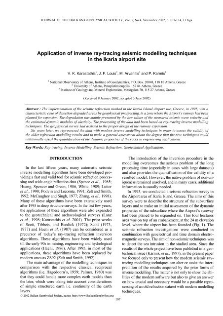
Application of inverse ray-tracing seismic modelling techniques

JOURNAL OF THE BALKAN GEOPHYSICAL SOCIETY, Vol. 5, No 4, November 2002, p. 107-114, 11 figs.
Application of inverse ray-tracing seismic modelling techniques
in the Ikaria airport site
V. K. Karastathis 1 , J. F. Louis 2 , M. Arvanitis 2 and P. Karmis 3
1 National Observatory of Athens, Institute of Geodynamics, P.O. Box. 20048, 118 10 Athens, Greece
2 University of Athens, Panepistimioupolis, 157 84 Athens, Greece
3 Institute of Geology and Mineral Exploration, Mesogeion 70, 115 27 Athens, Greece
(Received 9 January 2002; accepted 3 June 2002)
Abstract : The implementation of the seismic refraction method in the Ikaria Island Airport site, Greece, in 1995, was a
characteristic case of detection degraded areas by geophysical prospecting, in a zone where the Airport’s runway had been
planned for expansion. The degradation was mainly presumed by the low values of the measured seismic wave velocity and
the estimated dynamic modulus of elasticity. The processing of the data had been based on ray-tracing inverse modelling
techniques. The geophysical survey had assisted to the proper design of the runway expansion.
Six years later, we reprocessed the data with modern inverse modelling techniques in order to assess the validity of
the older refraction modelling results and to make a general assessment about the degree that the new techniques could
additionally assist the quantification of the dynamic properties of the rocks in engineering applications.
Key Words: Ray-tracing, Inverse Modelling, Seismic Refraction, Geotechnical Applications.
INTRODUCTION
In the last fifteen years, many automatic seismic
inverse modelling algorithms have been developed providing
a fast and valid tool for seismic refraction processing
and wide-angle reflection data (Spence et al., 1985;
Huang, Spencer and Green, 1986, White, 1989; Lutter
et al., 1990; Podvin and Lecomte, 1991; Zelt and Smith,
1992; McCaughey and Singh, 1977; Zhang, et al., 1998).
Many of these algorithms have been extensively used
after 1995 in deep structure surveys. In the last few years,
the applications of these algorithms were also expanded
to the geotechnical and archaeological surveys (Lanz
et al., 1998; Karastathis et al. 2001). The prior works
of Scott, Tibbets, and Burdick (1972); Scott (1973,
1977) and Haeni et al. (1987) can be considered as a
precursor of today’s ray-tracing refraction inversion
algorithms. These algorithms have been widely used
till the early 90s in mining, engineering and hydrological
applications (Haeni, 1986). After 1995, in most of the
applications, these algorithms have been replaced by
modern ones as ZS92 (Zelt and Smith, 1992).
The main advantage of the modelling techniques in
comparison with the respective classical reciprocal
algorithms (i.e. Hagedoorn’s, 1959; Palmer, 1980) was
that they could handle more complex earth models than
the later, which were taking into account considerations
of simple structured earth i.e. continuity of the earth
layers.
© 2002 Balkan Geophysical Society, access http://www.BalkanGeophySoc.org
107
The introduction of the inversion procedure in the
modelling overcomes the serious problem of the long
processing time (especially in cases with large datasets)
and also provides the quantification of the validity of a
resulted model. However, the native problem of non-uniqueness
remained unsolved, and in many cases, additional
information is usually needed.
In 1995, we conducted a seismic refraction survey in
the Airport area of Ikaria Island, Greece. The aims of this
survey were to describe the structure of the subsurface
layers and to make an initial assessment of the dynamic
properties of the subsurface where the Airport’s runway
had been planed to be expanded on. This four hectares
area was on top of an embankment, at the 24 m elevation
level, where the airport has been founded (Fig. 1). The
seismic refraction investigations were conducted in
combination with geoelectrical and time domain electromagnetic
surveys. The aim of non-seismic techniques was
to detect the sea intrusion in the studied area. Since the
results of the whole project have been published in a geotechnical
issue (Karmis, et al., 1997), in the present paper
we focused only to present how the modern seismic raytracing
modelling techniques can alter or assist the interpretation
of the results acquired by the prior forms of
inverse modelling. The matter is not only to show the abilities
of the modern software but also to give an answer
on how crucial and necessary would be a possible reprocessing
of an old refraction dataset with modern modelling
techniques.

108 Karastathis et al.
FIG. 1. The runway of the Ikaria airport is oriented NNE-SSW and terminated on an embankment area near the coast.
At this area the runway was planned to be extended. (photo: Air Traffic Safety Electronic Engineers Association of
Hellenic Civil Aviation Authority: http://www.hcaa-eleng.gr/ikaria.htm)
GEOLOGICAL SETTING
The bedrock that underlies the embankment is a metamorphosed
unit constituted by phyllite and schist, with
a succession of intercalated carbonate layers. Highly
fractured carbonate layers are observed on the outcrops.
The surface sediments consist of sand and pebble conglomerate.
The embankment material is made of scree and
boulders.
DATA ACQUISITION AND PROCESSING
A number of P-wave seismic refraction profiles were
conducted in the investigated area. Additional P-wave
refraction survey was carried out to estimate the Poisson
ratio of the bedrock in an adjacent area where the bedrock
outcropped. Some shorter S-wave refraction
profiles were also conducted in order to contribute to
the assessment of the dynamic properties of the layers.
The locations of the P-wave refraction profiles IKRP1,
IKRP2, IKRP3 and IKRP4 are shown in Figure 2. The
dataset IKRP1 was acquired with the use of 48 geophones
and spacing interval of 4 m. A 24 geophone layout
was used in all the other lines. The receiver interval was
4 m for IKRP2 and IKRP3 and 2 m for IKRP4. The
lengths of the IKRP1, IKRP2, IKRP3 and IKRP4 were
188, 92, 92 and 46 m respectively. Dynamite was used
as seismic source for the data acquisition and the resonant
frequency of geophones was 10 Hz. The data recording
unit was an ABEM Terraloc instrument.
The first processing of the data (Karmis et al., 1997)
was done by the use of the inversion ray-tracing modelling
algorithm SIPT1 of Haeni et al. (1987), based on
the previous work of Scott, Tibbets and Burdick (1972)
and Scott (1973, 1977). The program could handle mo-
FIG. 2. Sketch map of the P-wave refraction profiles.
dels with steeply dipping layers and abrupt changes in
velocity. Its ability for data processing was limited to 48
traces per shot and seven shots per spread. The algorithm
could support models only with five or less layers. The
inputs required by the program are the first arrival times,
the assignment of arrivals to the corresponding refractors
as well as the positions (elevation and location) of
the sources and receivers. By the use of a delay-time
method the program performs a first approximation of the

Application of inverse ray-tracing seismic modelling techniques ... 109
N
60 70 80 90 100 110 120 130 140 150 160 170 180 190 200 210 220 230 240
S
20
10
0
0.3 1.3 2.3 3.3 4.3
Km/s
FIG. 3. Velocity structure of the refraction profile IKRP1. Triangles denote geophone positions.
FIG. 4. Top: The first arrival ray-paths through a two-layer model of IKRP1. Bottom: Comparison of observed (bars
represent ±1.2 ms uncertainty) and predicted travel times shown by dots. Overall RMS misfit was 1.18 ms for 288 arrivals.
layered model. This initial model is improved by the implementation
of an automatic inversion procedure based
on a ray-tracing technique. In particular, a set of travel
times are calculated by the program, and compared with
the observed data and if the misfit is not within a userspecified
limit, the refractor interface is adjusted in a
such way to improve the model travel times fitting. The
procedure is iterative and is continued until the limit
was reached. The resulted model is finally smoothed.
The program Rayinvr (Zelt and Smith, 1992; Zelt and
Forsyth, 1994) was implemented for the reprocessing
of the data. This is a ray-tracing algorithm accompanied
with a least-square inversion routine that uses any type
of seismic wave arrivals and provides a simultaneous
determination of the 2-D velocity and interface structure.
It uses a layered model consisted of trapezoids cells. The
user defines the number and the shape of the trapezoid
cells and also sets the velocity values on their corners.
This definition is done by setting up the respective
“boundary” and “velocity nodes”. The velocity values
within the trapezoids come from a linear interpolation
between the four defined corner velocities. The algorithm
not only improves the time required for data processing
in comparison to the forward modelling but also
estimates model parameter resolution, uncertainty and
non-uniqueness. The Rayinvr has been mostly used in
crustal studies such as those reported by Zelt and Ellis
(1989); O’Leary, et al. (1995); Zelt and White (1995);
Clowes, et al.,(1995); and Sato and Kennett (2000). The
data processing was done on a Sun Ultra 10 workstation.

110 Karastathis et al.
4.6
4.1
3.6
3.1
2.6
2.1
1.6
1.1
0.6
0
-0.5
-1
-1.5
-2
-2.5
Km/s
-3 Km/s
20
10
0
20
10
0
20
10
0
20
10
0
20
10
0
20
10
0
100 150 200
100 150 200
100 150 200
100 150 200
100 150 200
100 150 200
FIG. 5. A single parameter resolution test. The final model (A) was perturbed by raising the 180 m node by 3 m. The
resulting model (B) was used to produce a new arrival time dataset. The inversion of the final model (A) with the
perturbed time dataset resulted to a new model (C). The next model (D) presents the initial perturbation which created the
perturbed time dataset. Model (E) shows the resulted perturbation on the final model crated by inverting the perturbed
time dataset. The models (D) and (E) are little different. The difference is shown in model (F).
A
B
C
D
E
F
N
60 70 80 90 100 110 120 130 140 150 160 170 180 190 200 210 220 230 240
S
20
10
0
0 5 10 15 20 25 30 35 40 45 50
GPa
FIG. 6. Section representing the estimated elasticity modulus of the line IKRP1.
FIG. 7. The refraction seismic section after processing with the SIPT1 algorithm.

Application of inverse ray-tracing seismic modelling techniques ... 111
1400
1200
1000
Velocity (m/s)
800
600
400
200
0
60 80 100 120 140 160 180 200 220 240
Distance (m)
FIG. 8. The horizontal variation of the overburden layer velocity as calculated by the algorithm SIPT1 on the IKRP1
data.
W
60 80 100 120 140
E
20
10
0
0.3 0.8 1.3 1.8 2.3 2.8 3.3 3.8 4.3 4.8
Km/s
20
W
60 70 80 90 100 110 120 130 140 150
E
10
0
0 3 6 9 12 15 18 21 24 27 30 33 36 39 42 45 48
GPa
FIG. 9. The velocity model (top) and the respective presentation of the estimated elasticity modulus (bottom) of the
seismic line IKRP2.

112 Karastathis et al.
1200
1000
800
Velocity (m/s)
600
400
200
0
60 80 100 120 140
Distance (m)
FIG. 10. The horizontal variation of the velocity of the overburden in IKRP2 line, as calculated by the algorithm SIPT1.
5 10 15 20 25 30 35 40 45
20
700 m/s 1000 m/s 1200 m/s
15
10
5
0.3 1.3 2.3 3.3 4.3
Km/s
FIG. 11. The velocity structure of the refraction profile IKRP4 as resulted from the processing with the Rayinvr algorithm.
The numbers inside indicate the velocity values as calculated by SIPT1.
RESULTS
The results of the seismic and geoelectical surveys
in 1995 (Louis and Karastathis, 1996; Karmis et al.,
1997), described a deteriorated zone at the eastern side
of the investigated area. Although seismic refraction
survey succeeded to detect this deterioration, questions
remained outstanding about the precision and the completeness
of the results. The comparison of the previous
results derived by the SIPT1 algorithm with the new
ones acquired by one of the most popular and modern
inversion modelling algorithms, the Rayinvr, provided
us with useful answers to all these questions.
The line IKRP1 could be considered as the backbone
line of the seismic survey. The model resulted after
processing with Rayinvr is presented in Figure 3. The
structure is simple without any abrupt anomaly in the
depth of the bedrock interface or in the P-wave velocity

Application of inverse ray-tracing seismic modelling techniques ... 113
values. The lowest values of the P-wave velocity of the
first layer (800 – 900 m/s) around 80-100 m and 130-
160 m are concentrated in very shallow depths and could
not lead to any concern about the compactness of this
layer. These low values can be attributed to a natural
deterioration of the superficial materials.
The ray-coverage of IKRP1 was dense enough to
describe the P-wave velocity of the first layer and the
upper part of the bedrock (See Figure 4 – upper panel).
This was succeeded by utilizing 48 geophones and 7
shots which are the maximum limits of the processing
capabilities of the SIPT algorithm. The fitting between
calculated and observed times was very good (Figure 4
– lower panel) since the RMS error was not higher than
1.2 ms.
We also tested the stability of the final model (Fig.
5a) by perturbing it at one point (180 m). Actually, we
moved the boundary node of this point upwards for 2 m.
The velocity model then was modified (Fig. 5b). A new
data set was created by forward modelling. This data
was inverted by using the final model as a starting model.
The inversion produces a new model (Fig. 5c). The
purpose was to check if the final model was sensitive
to small perturbations. We found out that the model
was stable, since the smearing around the anomaly was
very small. The resulted model after the inversion of
the perturbed data is shown in Figure 5c. Figure 5d
shows the initial perturbation of the model (difference
between 5a and 5b), the Figure 5e shows the resulted
anomaly (difference between 5a and 5c) and the Figure
5f shows the difference between the two anomalies (5d
and 5e). We can notice that the difference is very small
and we can conclude that the inversion is stable.
We also estimated the elastic modulus of the materials
in the IKRP1 section. The resulted section is shown
in Figure 6.
The comparison of the new results with the previous
ones showed a very good agreement in the depth estimation
of the bedrock. Figure 7 shows the refraction
profile as resulted from the SIPT1 processing. The
velocity distribution of the first layer is presented in
Figure 8. The estimated velocity values by SIPT1 (see
Fig. 8) agreed well with the values of the first six meters
material in the Rayinvr model. This was expected since
the major part of the first layer rays came through these
first meters. If Karmis et al., (1997) had not conducted
supplementary geophysical methods such as geoelectrical
profiling or electromagnetic soundings, they could
not be able to evaluate the quality of the interpretation
for the layers deeper than 5-6 m. The modern modelling
technique able to handle models with linear velocity
increase allowed estimating velocity at those depths.
The deteriorated area at the eastern part of the
investigated area was detected by both the IKRP2 and
IKRP3 lines. We present P-wave velocity and elasticity
modulus sections obtained from the modelling of line
IKRP2 profile (Fig. 9). It is easily seen that the area over
120 m has lower values of P-wave velocity. Figure 10
shows the velocity graph of the previous processing.
Although the velocity variation is clear in this section,
it is difficult to decide if the low velocity zone is limited
inside the upper layer without additional information.
Seismic line IKRP4 (Figure 11) also indicates a
small deterioration in the upper part of the first layer.
The estimated velocities by the previous processing are
presented by red lettering. The agreement between the
two processing methods as far as the P-wave velocity
is concerned, was very good. However the new processing
succeeded to specify better the area with the lower
velocities.
CONCLUSIONS
The reprocessing of the data leads to obtain new
information about the velocity field derived from the
seismic refraction survey. It also provides an idea about
the quality of the previous inverse modelling results.
The former techniques could not estimate the velocity
values in the deeper part of the upper layer since they
could not handle models with a gradient increase in the
velocity field.
The reprocessing of the data is worth trying since
new information can be derived from the former seismic
refraction experiments having extensive ray-coverage.
In Greece, there are many datasets i.e. important engineering
seismic surveys and crustal investigations. This
work shows that the reinterpretation of these datasets
would be very useful.
REFERENCES
Clowes, R. M., Zelt, C. A., Amor, J. R. and Ellis, R. M., 1995.
Lithospheric structure in the southern Canadian Cordillera from a
network of seismic refraction lines: Can. J. Earth Sci., 32, 1485–
1513.
Haeni, F. P., 1986. Application of seismic-refraction techniques to
hydrologic studies: U.S. Geological Survey Open File Report
84-746, 144.
Haeni, F. P., Grantham D. G., and Ellefsen K., 1987. Micro-computer-based
version of SIPT-. A program for interpretation of
seismic refraction data: U.S. Geological Survey Open file report
87-103-A. Hartford, Connecticut.
Hagedoorn J. G., 1959. The plus-minus method of interpreting
seismic refraction sections: Geophysical Prospecting, 7, 158-182.
Huang, H., Spencer, C. and Green, A., 1986. A method for the
inversion of refraction and reflection travel times for laterally
varying velocity structures: Bull. Seism. Soc. Am., 76 , 837-846.
Karastathis, V. K., Papamarinopoulos S. and Jones R. E., 2001.
2-D velocity structure of the buried ancient canal of Xerxes:
An application of seismic methods in archaeology: Journal of
Applied Geophysics, 47, 29–43
Karmis P., Louis J. F. and Karastathis V. K., 1997. Site characterisation
by geophysical methods - A case history: Proceedings,
International Symposium on Engineering Geology and the Environment
- Greek National Group of International Association
of Engineering Geology (IAEG), Athens, 1997, 1285 - 1291.

114 Karastathis et al.
Lanz, E., Maurer, H., and Green, A. G., 1998. Refraction tomography
over a buried waste disposal site: Geophysics, 63, 1414-1433.
Louis J. F. and Karastathis V. K., 1996. Seismic investigations in
Ikaria airport: Technical Report. University of Athens.
Lutter, W. J., Nowack, R. L., and Braile, L. W., 1990. Seismic
imaging of upper crustal structure using travel times from the
PASSCAL Ouachita experiment: J. Geophys. Res., 95, 4621-4631.
McCaughey, M., and Singh, S. C., 1997. Simultaneous velocity and
interface tomography of normal-incidence and wide-aperture
traveltime data: Geophys. J. Int., 131, 87-99.
O’Leary, D. M., Ellis, R. M., Stephenson, R. A., Lane, L. S., and
Zelt, C. A., 1995. Crustal structure of the northern Yukon and
MacKenzie Delta: J. Geophys. Res. 100, 9905–9920.
Palmer, D., 1980. The generalized reciprocal method of seismic
refraction interpretation. Society of Exploration Geophysicists.
Podvin, P., and Lecomte, I., 1991. Finite-difference computation
of traveltimes in very contrasted velocity models: A massively
parallel approach and its associated tools: Geophys. J. Internat.,
105, 271–284.
Sato, Τ., and Kennett B. L. N., 2000. Two-dimensional inversion
of refraction traveltimes by progressive model development:
Geophys. J. Int., 140, 543-558.
Scott, J. H., 1977. SIPT – a seismic refraction inverse modelling program
for timeshare terminal computer systems: U.S. Geological
Survey Open File Report 77-365, 35 pp.
Scott, J. H., Tibbets, B. L., and Burdick, R. G., 1972. Computer
analysis of seismic refraction data: U.S. Bureau of Mines, Report
Investigations, 7595, 95.
Scott, J. H., 1973. Seismic refraction modelling by computer: Geophysics,
38, 271-284.
Spence, G. D., Clowes, R. M., and Ellis, R. M., 1985. Seismic
structure across the active subduction zone of western Canada:
J. Geophys. Res., 90, 6754-6772.
White, D. J., 1989. Two-dimensional seismic refraction tomography:
Geophys. J. Int., 97, 223-245.
Zelt, C. A. and Forsyth, D. A., 1994. Modelling wide-angle seismic
data for crustal structure: southeastern Grenville province: J.
Geophys. Res., 99, 11687-11704.
Zelt, C. A. and Smith, R. B., 1992. Seismic traveltime inversion
for 2-D crustal velocity structure: Geophys. J. Int., 108, 16-34.
Zelt, C. A., Ellis, R. M., 1989. Seismic structure of the crust and
upper mantle in the Peace River Arch region: Can. J. Geophys.
Res., 94, 5729–5744.
Zelt, C. A., White, D. J., 1995. Crustal structure and tectonics of
the southeastern Canadian Cordillera: J. Geophys. Res., 100,
24255–24273.
Zhang, J., ten Brink, U.S. and Toksφz, M.N., 1998. Nonlinear
refraction and reflection traveltime tomography: J. Geophys.
Res., 103, 29743-29757.