Application of inverse ray-tracing seismic modelling techniques

110 Karastathis et al.
4.6
4.1
3.6
3.1
2.6
2.1
1.6
1.1
0.6
0
-0.5
-1
-1.5
-2
-2.5
Km/s
-3 Km/s
20
10
0
20
10
0
20
10
0
20
10
0
20
10
0
20
10
0
100 150 200
100 150 200
100 150 200
100 150 200
100 150 200
100 150 200
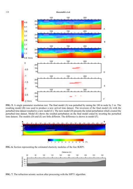
FIG. 5. A single parameter resolution test. The final model (A) was perturbed by raising the 180 m node by 3 m. The
resulting model (B) was used to produce a new arrival time dataset. The inversion of the final model (A) with the
perturbed time dataset resulted to a new model (C). The next model (D) presents the initial perturbation which created the
perturbed time dataset. Model (E) shows the resulted perturbation on the final model crated by inverting the perturbed
time dataset. The models (D) and (E) are little different. The difference is shown in model (F).
A
B
C
D
E
F
N
60 70 80 90 100 110 120 130 140 150 160 170 180 190 200 210 220 230 240
S
20
10
0
0 5 10 15 20 25 30 35 40 45 50
GPa
FIG. 6. Section representing the estimated elasticity modulus of the line IKRP1.
FIG. 7. The refraction seismic section after processing with the SIPT1 algorithm.