solutions - UBC Mechanical Engineering

Foundations in Control Engineering (MECH550P-201)
Final exam (50 points). April 17, 3:30pm–6pm
Sketch of solutions
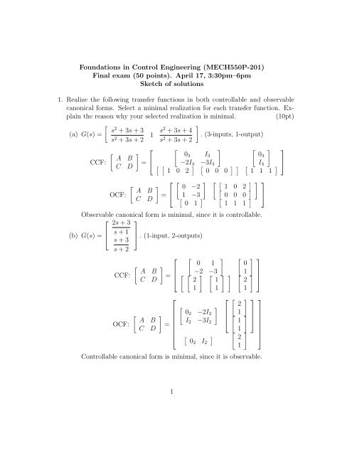
1. Realize the following transfer functions in both controllable and observable
canonical forms. Select a minimal realization for each transfer function. Explain
the reason why your selected realization is minimal.
(10pt)
[ ]
s
(a) G(s) =
2 + 3s + 3
s 2 + 3s + 2 1 s2 + 3s + 4
. (3-inputs, 1-output)
s 2 + 3s + 2
⎡ [ ] [ ] ⎤
[ ]
03 I A B
3
03
CCF:
= ⎣ −2I
C D [ [ 3 −3I 3 I 3
⎦
] [ ] ] [ ]
1 0 2 0 0 0 1 1 1
OCF:
[ A B
C D
⎡
]
= ⎣
[ ] [ [ ]
0 −2
[ 1 0 2
]
[
1 −3
] [ 0 0 0
]
0 1 1 1 1
]
⎤
⎦
Observable canonical form is minimal, since it is controllable.
⎡
2s + 3
⎤
⎢ s + 1 ⎥
(b) G(s) = ⎣ ⎦ . (1-input, 2-outputs)
s + 3
s + 2
⎡
] ⎤
[ ] A B
CCF:
=
C D
⎢
⎣
[ ] [ 0 1 0
[ [
−2
] [
−3
] ] [
1
]
2 1 2
1 1 1
⎥
⎦
OCF:
[ A B
C D
⎡
]
=
⎢
⎣
[ ]
02 −2I 2
I 2 −3I 2
[
02 I 2
]
⎡
⎢
⎣
[ 2
1
[ 1
1
[ 2
1
]
]
]
⎤
⎥
⎦
⎤
⎥
⎦
Controllable canonical form is minimal, since it is observable.
1

2. Consider a system: ⎧
⎪⎨
⎪ ⎩
ẋ(t) =
[ 0 2
1 −1
]
x(t),
y(t) = [ 1 1 ] x(t).
For each of the following specified locations of the observer poles:
• eig(A − LC) = −2, −3.
• eig(A − LC) = −3, −3.
• eig(A − LC) = −1 ± j.
is it possible to design an observer? If the answer is “yes”, design an observer.
For the system given above, what is the condition for given observer pole
locations to be achievable?
(10pt)
By the direct method,
det(λI − (A − LC)) = · · · = (λ + 2)(λ + l 1 + l 2 − 1).
Therefore, for whatever choice of L, the eigenvalue of s = −2 is impossible
to move. Thus, the first observer poles are possible to achieve with L such
that l 1 + l 2 = 4, but other two observer poles are not possible to achieve.
The condition for given observer pole locations to be achievable is that they
include s = −2.
3. Consider a system {
ẋ(t) = αx(t) + u(t),
y(t) = x(t).
(a) For α = −1, design a state feedback with an integrator such that the
closed-loop poles are s = −1, −1.
(10pt)
det(λI−(A aug −B aug
[
K
Ka
]
) = · · · = λ 2 +(K−α)λ−K a = λ 2 +2λ+1
When α = −1, K = 1 and K a = −1.
(b) Suppose that our modeling is inaccurate and that the actual α is not −1.
For the designed controller in (a), what is the range of the parameter
α that results in zero steady-state tracking error for any step reference
input?
(10pt)
For the designed controller parameters K = 1 and K a = −1, α must be
less than one to keep the closed-loop stability.
2

4. Solve the following continuous-time infinite-horizon LQR problem: (10pt)
min
u(·)
∫ ∞
0
subject to
(
x
2
1 (t) + u 2 (t) ) dt,
[
ẋ1 (t)
ẋ 2 (t)
]
=
[ 0 1
0 −1
] [
x1 (t)
x 2 (t)
] [ 0
+
1
]
u(t).
Verify the stability of the closed-loop system.
Algebraic Riccati equation:
[ √ ] 3 1
A T P + P A − P BR −1 B T P + Q = 0 ⇒ P = √ > 0
1 3 − 1
u(t) = −R −1 B T P x(t) = − [ 1
√ 3 − 1 ] x(t)
The closed-loop system is stable since
A cl := A − BR −1 B T P =
[ 0 1
−1 − √ 3
]
3