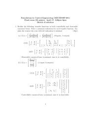
DT Kalman filter - UBC Mechanical Engineering - University of ...
DT Kalman filter - UBC Mechanical Engineering - University of ...
DT Kalman filter - UBC Mechanical Engineering - University of ...

You also want an ePaper? Increase the reach of your titles
YUMPU automatically turns print PDFs into web optimized ePapers that Google loves.
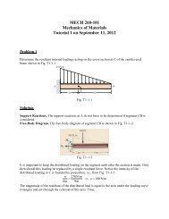
MECH468<br />
Modern Control <strong>Engineering</strong><br />
MECH550P<br />
Foundations in Control <strong>Engineering</strong><br />
Lecture 30<br />
Duality, Steady-state<br />
<strong>Kalman</strong> <strong>filter</strong><br />
LQG, Summary <strong>of</strong> the course<br />
Dr. Ryozo Nagamune<br />
Department <strong>of</strong> <strong>Mechanical</strong> <strong>Engineering</strong><br />
<strong>University</strong> <strong>of</strong> British Columbia<br />
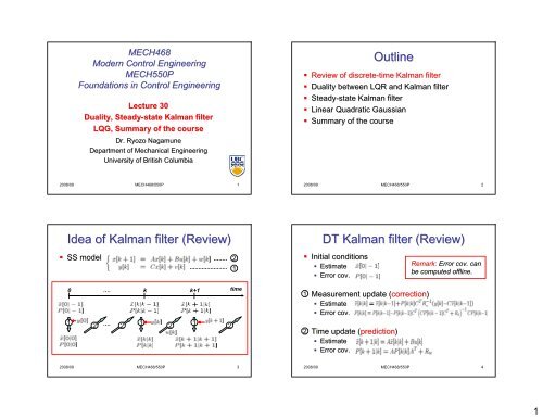
Outline<br />
• Review <strong>of</strong> discrete-time<br />
time <strong>Kalman</strong> <strong>filter</strong><br />
• Duality between LQR and <strong>Kalman</strong> <strong>filter</strong><br />
• Steady-state<br />
<strong>Kalman</strong> <strong>filter</strong><br />
• Linear Quadratic Gaussian<br />
• Summary <strong>of</strong> the course<br />
2008/09 MECH468/550P 1<br />
2008/09 MECH468/550P 2<br />
Idea <strong>of</strong> <strong>Kalman</strong> <strong>filter</strong> (Review)<br />
• SS model<br />
2<br />
1<br />
<strong>DT</strong> <strong>Kalman</strong> <strong>filter</strong> (Review)<br />
• Initial conditions<br />
• Estimate<br />
• Error cov.<br />
Remark: Error cov. . can<br />
be computed <strong>of</strong>fline.<br />
0<br />
1<br />
2<br />
….<br />
k k+1<br />
time<br />
…. 2<br />
1<br />
2<br />
1<br />
2<br />
1<br />
2<br />
Measurement update (correction(<br />
correction)<br />
• Estimate<br />
• Error cov.<br />
Time update (prediction(<br />
prediction)<br />
• Estimate<br />
• Error cov.<br />
2008/09 MECH468/550P 3<br />
2008/09 MECH468/550P 4<br />
1
One-step<br />
<strong>Kalman</strong> <strong>filter</strong> (review)<br />
Outline<br />
• Review <strong>of</strong> discrete-time<br />
time <strong>Kalman</strong> <strong>filter</strong><br />
• Duality between LQR and <strong>Kalman</strong> <strong>filter</strong><br />
• Steady-state<br />
<strong>Kalman</strong> <strong>filter</strong><br />
• Linear Quadratic Gaussian<br />
• Summary <strong>of</strong> the course<br />
• Gain<br />
2008/09 MECH468/550P 5<br />
2008/09 MECH468/550P 6<br />
Duality between LQR and KF<br />
• <strong>DT</strong> LQR<br />
Backward computation<br />
• <strong>Kalman</strong> <strong>filter</strong><br />
Outline<br />
• Review <strong>of</strong> discrete-time<br />
time <strong>Kalman</strong> <strong>filter</strong><br />
• Duality between LQR and <strong>Kalman</strong> <strong>filter</strong><br />
• Steady-state<br />
<strong>Kalman</strong> <strong>filter</strong><br />
• Linear Quadratic Gaussian<br />
• Summary <strong>of</strong> the course<br />
Forward computation<br />
Mathematically dual!<br />
2008/09 MECH468/550P 7<br />
2008/09 MECH468/550P 8<br />
2
Remarks on <strong>Kalman</strong> <strong>filter</strong> (KF)<br />
• <strong>Kalman</strong> (<strong>filter</strong>) gain is time-varying, but it<br />
typically reaches the steady state quickly,<br />
because P[k|k-1] reaches steady state quickly.<br />
• To simplify implementation <strong>of</strong> KF, it is <strong>of</strong>ten<br />
preferable to use a constant-gain KF.<br />
• In many cases, this does not degrade the <strong>filter</strong><br />
performance.<br />
• How to obtain such steady state <strong>Kalman</strong> gain?<br />
• We need an assumption: (A,C) observable<br />
Steady-state<br />
<strong>Kalman</strong> gain<br />
• For time-varying<br />
<strong>Kalman</strong> gain, we solve an<br />
equation recursively to obtain error covariances.<br />
• By omitting “k” to find the equation for steady<br />
state, and by setting<br />
Discrete Algebraic Riccati Equation<br />
2008/09 MECH468/550P 9<br />
2008/09 MECH468/550P 10<br />
SS <strong>Kalman</strong> gain in Matlab<br />
• dare.m<br />
Steady-state<br />
<strong>Kalman</strong> <strong>filter</strong><br />
• Initial conditions<br />
• Estimate<br />
• Error cov.<br />
Replace<br />
(Steady state <strong>of</strong> P[k|k])<br />
1<br />
Measurement update<br />
• Estimate<br />
• Error cov.<br />
• dlqe.m<br />
(Steady state <strong>of</strong> P[k+1|k])<br />
(Steady state <strong>of</strong> P[k|k])<br />
2<br />
Time update<br />
• Estimate<br />
• Error cov.<br />
2008/09 MECH468/550P 11<br />
2008/09 MECH468/550P 12<br />
3
• Gain<br />
One-step steady-state state KF<br />
FACT<br />
2008/09 MECH468/550P 13<br />
More on <strong>Kalman</strong> <strong>filter</strong><br />
• Books<br />
• D.Simon, “Optimal State Estimation”, , John Wiley & Sons,<br />
2006<br />
• R.F.Stengel, “Optimal Control and Estimation”, , Dover<br />
Publications, 1994<br />
• B.D.O.Anderson and J.Moore, “Optimal Filtering”, , Dover<br />
Publications, 2005<br />
• Websites<br />
• Greg Welch and Gary Bishop<br />
http://www.cs.unc.edu/~welch/kalman/index.html<br />
• Peter Joseph<br />
http://ourworld.compuserve.com/homepages/PDJoseph/<br />
2008/09 MECH468/550P 14<br />
Outline<br />
• Review <strong>of</strong> discrete-time<br />
time <strong>Kalman</strong> <strong>filter</strong><br />
• Duality between LQR and <strong>Kalman</strong> <strong>filter</strong><br />
• Steady-state<br />
<strong>Kalman</strong> <strong>filter</strong><br />
• Linear Quadratic Gaussian<br />
• Summary <strong>of</strong> the course<br />
<strong>DT</strong> finite-horizon LQR (review)<br />
• Problem<br />
• J : Quadratic performance index (cost function)<br />
For small state<br />
• Design parameters<br />
For small input<br />
For small final state<br />
2008/09 MECH468/550P 15<br />
2008/09 MECH468/550P 16<br />
4
LQR optimal control law (review)<br />
• LQR optimal control:<br />
Stochastic LQR with measured x<br />
• Optimization problem<br />
• P[k]: positive semidefinite solution to a matrix Riccati<br />
difference equation<br />
• w : white, zero mean, Gaussian<br />
• J : Quadratic performance index (cost function)<br />
Expected value over<br />
Optimal control law is exactly the same as in the previous slide!<br />
2008/09 MECH468/550P 17<br />
2008/09 MECH468/550P 18<br />
LQG (Linear Quadratic Gaussian)<br />
• Problem<br />
• x[0] : Gaussian<br />
• w,v : white, Gaussian<br />
• x[0],w,v : uncorrelated<br />
• x : not available<br />
• J : Quadratic performance index (cost function)<br />
LQG optimal control<br />
• Optimal control law = LQR + <strong>Kalman</strong> <strong>filter</strong><br />
lqgreg.m<br />
Expected value over<br />
dlqr.m<br />
dlqe.m<br />
2008/09 MECH468/550P 19<br />
2008/09 MECH468/550P 20<br />
5
Remarks<br />
• Separation principle holds! Thus, we can design LQR<br />
controller and <strong>Kalman</strong> <strong>filter</strong> independently.<br />
• The feedback structure is same as observer-based<br />
based<br />
control. Thus, in infinite horizon LQR plus steady state<br />
KF cases, the eigenvalues <strong>of</strong> closed-loop loop A-matrix A<br />
consists <strong>of</strong> the A-matrix A<br />
<strong>of</strong> LQR feedback system with full<br />
state feedback, and the A-matrix A<br />
<strong>of</strong> <strong>Kalman</strong> <strong>filter</strong>.<br />
• Recall that LQR has a good robust stability property<br />
expressed by gain and phase margin (in SISO cases).<br />
However, it is known that LQG may possibly lose such<br />
good property (Doyle & Stein). This fact motivated<br />
development <strong>of</strong> robust control theory.<br />
Outline<br />
• Review <strong>of</strong> discrete-time<br />
time <strong>Kalman</strong> <strong>filter</strong><br />
• Duality between LQR and <strong>Kalman</strong> <strong>filter</strong><br />
• Steady-state<br />
<strong>Kalman</strong> <strong>filter</strong><br />
• Linear Quadratic Gaussian<br />
• Summary <strong>of</strong> the course<br />
2008/09 MECH468/550P 21<br />
2008/09 MECH468/550P 22<br />
Systematic controller design process<br />
Reference<br />
Controller<br />
Actuator<br />
Input<br />
Disturbance<br />
Plant<br />
Output<br />
Control and estimation <strong>of</strong> states<br />
“State” has been the key concept in this course!<br />
Control<br />
Estimation<br />
4. Implemenation<br />
Controller<br />
3. Design<br />
Sensor<br />
1. Modeling<br />
Mathematical model<br />
2. Analysis<br />
2008/09 MECH468/550P 23<br />
System<br />
• Controllability & Observability<br />
• State feedback & Observer<br />
• Linear quadratic regulator & <strong>Kalman</strong> <strong>filter</strong><br />
Duality between control and estimation!<br />
2008/09 MECH468/550P 24<br />
6
Goals <strong>of</strong> the course (1 st lecture)<br />
To learn control theory with linear state-space space models<br />
• Modeling as a state-space space model<br />
• Differential or difference equation (instead <strong>of</strong> TF)<br />
• Linear algebra (instead <strong>of</strong> Laplace transform)<br />
• Analysis<br />
• Stability, controllability, observability<br />
• Realization, minimality<br />
• Design<br />
• State feedback, observer<br />
• Linear Quadratic Regulator (LQR), <strong>Kalman</strong> Filter<br />
• Matlab simulation<br />
2008/09 MECH468/550P 25<br />
Brief history <strong>of</strong> Control <strong>Engineering</strong><br />
• Classical control (-1950)(<br />
• Transfer function<br />
• Frequency domain<br />
• Modern control (1960-) ) (contents in this course)<br />
• State-space model<br />
• Time domain<br />
• Optimality<br />
• Post-modern control (1980-)<br />
• Robust control<br />
• Hybrid control, etc.<br />
2008/09 MECH468/550P 26<br />
Advanced control theory<br />
• Nonlinear control<br />
• Optimal control<br />
• Robust control<br />
• Adaptive control<br />
• Digital control<br />
• Hybrid control<br />
• Intelligent control<br />
• System identification<br />
Relevant to the material<br />
in this course<br />
(Foundations<br />
in Control <strong>Engineering</strong>)<br />
<strong>Mechanical</strong> engineering<br />
Electrical engineering<br />
Chemical engineering<br />
Civil engineering<br />
Aerospace engineering<br />
Computer<br />
Physics<br />
Summary<br />
Control engineering supports various disciplines!<br />
Environmental engineering<br />
Computer engineering<br />
Mechatronics<br />
Nanotechnology<br />
Medicine, Economics, Biology<br />
Model<br />
Control <strong>Engineering</strong><br />
Hardware<br />
(Sensors & actuators)<br />
Chemistry<br />
Mathematics<br />
2008/09 MECH468/550P 27<br />
2008/09 MECH468/550P 28<br />
7
Homework (Due Apr 8, 5pm)<br />
• (Last one!) 5-2: 5<br />
Consider the following<br />
continuous-time time system (oscillator):<br />
Design the <strong>Kalman</strong> <strong>filter</strong> for the discrete-time<br />
time<br />
system obtained by sampling the system above<br />
with sampling time 0.5:<br />
2008/09 MECH468/550P 29<br />
Homework (cont’d)<br />
• Assumptions<br />
• E{w}=<br />
}=E{v}=0,<br />
Rw=0.01,<br />
Rv=0.04<br />
• Initial value <strong>of</strong> error covariance matrix M=I2.<br />
• u[k] ] is a square-wave function defined in<br />
KFoscillator.m.<br />
• Task: Modify KFoscillator.m, , and design both<br />
time-varying and steady state <strong>Kalman</strong> <strong>filter</strong>s.<br />
(You do not have to follow the provided m-file.) m<br />
• Verify that your steady state <strong>Kalman</strong> <strong>filter</strong> gain<br />
matches with the time-varying gain after some time.<br />
• Compare the trajectories <strong>of</strong> the state estimates.<br />
2008/09 MECH468/550P 30<br />
8