Review & today's topics State feedback - UBC Mechanical ...
Review & today's topics State feedback - UBC Mechanical ...
Review & today's topics State feedback - UBC Mechanical ...

You also want an ePaper? Increase the reach of your titles
YUMPU automatically turns print PDFs into web optimized ePapers that Google loves.
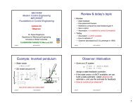
MECH468<br />
Modern Control Engineering<br />
MECH550P<br />
Foundations in Control Engineering<br />
Lecture 21<br />
<strong>State</strong> <strong>feedback</strong> design<br />
Lyapunov equation method<br />
Dr. Ryozo Nagamune<br />
Department of <strong>Mechanical</strong> Engineering<br />
University of British Columbia<br />
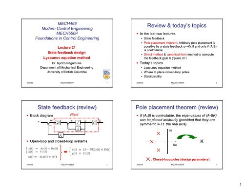
<strong>Review</strong> & today’s s <strong>topics</strong><br />
• In the last two lectures<br />
• <strong>State</strong> <strong>feedback</strong><br />
• Pole placement theorem: : Arbitrary pole placement is<br />
possible by a state <strong>feedback</strong> u=-Kx<br />
if and only if (A,B)<br />
is controllable<br />
• Direct method & canonical form method to compute<br />
the <strong>feedback</strong> gain K (“place.m(<br />
place.m”)<br />
• Today’s s <strong>topics</strong><br />
• Lyapunov equation method<br />
• Where to place closed-loop loop poles<br />
• Stabilizability<br />
2008/09 MECH468/550P 1<br />
2008/09 MECH468/550P 2<br />
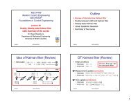
<strong>State</strong> <strong>feedback</strong> (review)<br />
• Block diagram<br />
Plant<br />
Pole placement theorem (review)<br />
• If (A,B) is controllable, the eigenvalues of (A-BK)<br />
can be placed arbitrarily (provided that they are<br />
symmetric w.r.t. . the real axis).<br />
Im<br />
• Open-loop and closed-loop loop systems<br />
Re<br />
K<br />
: Closed-loop loop poles (design parameters)<br />
2008/09 MECH468/550P 3<br />
2008/09 MECH468/550P 4<br />
1
<strong>Review</strong> & today’s s <strong>topics</strong><br />
• In the last two lectures<br />
• <strong>State</strong> <strong>feedback</strong><br />
• Pole placement theorem: Arbitrary pole placement is<br />
possible by a state <strong>feedback</strong> u=-Kx<br />
if and only if (A,B)<br />
is controllable<br />
• Direct method & canonical form method to compute<br />
the <strong>feedback</strong> gain K (“place.m(<br />
place.m”)<br />
• Today’s s <strong>topics</strong><br />
• Lyapunov equation method<br />
• Where to place closed-loop loop poles<br />
• Stabilizability<br />
2008/09 MECH468/550P 5<br />
Lyapunov equation method<br />
Step 0: Check if (A,B) is controllable. If it is, go to<br />
Step 1.<br />
Step 1: Select a matrix F with desired eigenvalues<br />
s.t.<br />
Step 2: Select a matrix<br />
Step 3: Solve the Lyapunov equation w.r.t. . T<br />
Step 4: If T is singular, redo from Step 3 with<br />
different<br />
Step 5: If T is nonsingular,<br />
2008/09 MECH468/550P 6<br />
Remarks on Lyapunov eq. . method<br />
• How to construct F<br />
• Suppose that the desired closed-loop loop poles are<br />
Idea of Lyapunov eq. . method<br />
• From Steps 3 & 5,<br />
Then, F can be chosen as<br />
• If T is nonsingular<br />
• How to construct : Select randomly!<br />
• Condition for the unique solution of the<br />
Lyapunov equation:<br />
• Conditions<br />
are necessary for the Lyapunov equation to<br />
have a nonsingular solution. (Proof omitted.)<br />
2008/09 MECH468/550P 7<br />
2008/09 MECH468/550P 8<br />
2
• SS model<br />
An example<br />
DC motor position control<br />
http://www.engin.umich.edu/group/ctm/examples<br />
www.engin.umich.edu/group/ctm/examples/<br />
• CL poles<br />
• Step 1:<br />
• Step 2:<br />
• Step 3:<br />
• Step 5:<br />
2008/09 MECH468/550P 9<br />
2008/09 MECH468/550P 10<br />
DC motor position control (cont’d)<br />
• <strong>State</strong>-space model<br />
2008/09 MECH468/550P 11<br />
DC motor position control (cont’d)<br />
• Specifications: For<br />
• r(t)=0<br />
• Settling time < 40 ms<br />
• Overshoot < 16%<br />
• Zero steady state error<br />
• Open-loop system<br />
• Poles = 0, -59.226<br />
-1.4545E+6<br />
• Not asymptotically stable!<br />
1<br />
0 0.02 0.04 0.06 0.08 0.1<br />
Time (sec)<br />
Feedback control for stability & performance!<br />
Position (rad)<br />
2008/09 MECH468/550P 12<br />
1.02<br />
1.015<br />
1.01<br />
1.005<br />
y(t) ) does not<br />
go to zero!<br />
3
Position (rad)<br />
1<br />
0.5<br />
0<br />
<strong>State</strong> <strong>feedback</strong> position control<br />
-0.5<br />
0 0.02 0.04 0.06 0.08 0.1<br />
Time (sec)<br />
Control input (volt)<br />
10<br />
0<br />
-10<br />
0 0.02 0.04 0.06 0.08 0.1<br />
Time (sec)<br />
Position (rad)<br />
1<br />
0.5<br />
0<br />
-0.5<br />
0 0.02 0.04 0.06 0.08 0.1<br />
Time (sec)<br />
Control input (volt)<br />
As the pole is moved away from the real axis, the overshoot<br />
becomes larger and the response becomes faster.<br />
10<br />
0<br />
-10<br />
0 0.02 0.04 0.06 0.08 0.1<br />
Time (sec)<br />
Exercise<br />
• Try the simulation by yourselves! (Matlab(<br />
code is<br />
on the course homepage.) Change the pole<br />
location, and get a feeling how responses are<br />
affected by the pole location.<br />
• For the system below, design a state <strong>feedback</strong><br />
u=-Kx<br />
so that the closed-loop loop system has -11 and<br />
-22 as its eigenvalues, , by Lyapunov eq. . method.<br />
2008/09 MECH468/550P 13<br />
2008/09 MECH468/550P 14<br />
<strong>Review</strong> & today’s s <strong>topics</strong><br />
• In the last two lectures<br />
• <strong>State</strong> <strong>feedback</strong><br />
• Pole placement theorem: Arbitrary pole placement is<br />
possible by a state <strong>feedback</strong> u=-Kx<br />
if and only if (A,B)<br />
is controllable<br />
• Direct method & canonical form method to compute<br />
the <strong>feedback</strong> gain K (“place.m(<br />
place.m”)<br />
• Today’s s <strong>topics</strong><br />
• Lyapunov equation method<br />
• Where to place closed-loop loop poles<br />
• Stabilizability<br />
2008/09 MECH468/550P 15<br />
Rules of thumbs<br />
• Move the poles for improvement of stability and<br />
performance.<br />
• Do not try to move poles farther than necessary.<br />
• Control input should not be too large.<br />
(desired CL) – (OL)<br />
• Place the poles in similar distances from the<br />
origin, , to make the control effort efficient.<br />
• Control effort depends on the farthest poles, while<br />
speed depends on the closest poles to the origin.<br />
2008/09 MECH468/550P 16<br />
4
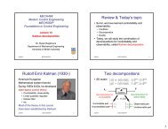
Butterworth configuration<br />
• 1930 Stephen Butterworth<br />
<strong>Review</strong> & today’s s <strong>topics</strong><br />
• In the last two lectures<br />
• <strong>State</strong> <strong>feedback</strong><br />
• Pole placement theorem: Arbitrary pole placement is<br />
possible by a state <strong>feedback</strong> u=-Kx<br />
if and only if (A,B)<br />
is controllable<br />
• Direct method & canonical form method to compute<br />
the <strong>feedback</strong> gain K (“place.m(<br />
place.m”)<br />
• Today’s s <strong>topics</strong><br />
• Lyapunov equation method<br />
• Where to place closed-loop loop poles<br />
• Stabilizability<br />
2008/09 MECH468/550P 17<br />
2008/09 MECH468/550P 18<br />
Stabilizability<br />
• Suppose that (A,B) is NOT controllable.<br />
• If the “uncontrollable part” of A-matrix A<br />
is stable,<br />
then the system is called stabilizable.<br />
Controllable pair<br />
Eigenvalues of this cannot be changed by state <strong>feedback</strong>.<br />
Summary<br />
• <strong>State</strong> <strong>feedback</strong><br />
• Lyapunov eq. . method to design state <strong>feedback</strong> gain<br />
• Where to place closed-loop loop poles (one always needs<br />
trial-and<br />
and-error)<br />
• Rules of thumbs<br />
• Butterworth configuration<br />
• Optimal method (We will learn more later in LQR.)<br />
• Stabilizability<br />
• Next,<br />
• Tracking (servo) control<br />
2008/09 MECH468/550P 19<br />
2008/09 MECH468/550P 20<br />
5
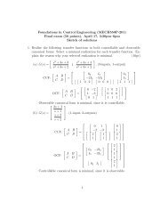
Homework<br />
• 4-1: For the inverted pendulum model in<br />
Homework 2-32<br />
3 (see slides for Lecture 10),<br />
design a state <strong>feedback</strong> controller.<br />
• Initial condition<br />
• The cart stops at y=0 with the upright pendulum.<br />
• The settling time should be at most 5 sec.<br />
• The input should be less than 15N all the time.<br />
Plot the trajectories of states and input by, for<br />
example, Simulink or lsim.m.<br />
2008/09 MECH468/550P 21<br />
6