Unsaturated Soil Mechanics as a Series of Partial Differential ...

Proceedings of International Conference on Problematic Soils, 25-27 May 2005,
Eastern Mediterranean University, Famagusta, N. Cyprus
Unsaturated Soil Mechanics as a Series of Partial
Differential Equations
Fredlund, D.G. 1 , Gitirana Jr., G. 2
1 Professor Emeritus, University of Saskatchewan, Saskatoon, SK, Canada
2 Ph.D. Student, University of Saskatchewan, Saskatoon, SK, Canada
Abstract
Unsaturated soil mechanics theory can be laid out as a series of governing partial differential
equations (PDEs). Formulations based on PDEs allow the solution of complex problems.
Examples include the analysis of volume change of expansive and collapsible soils, the design
of soil cover systems, and the analysis of transient slope stability. The practical relevance of
design approaches based on PDEs has increased as a result of recent advances in computer
geotechnics and the rise of problem solving environments, PSEs. However, the effective use
PSEs requires the ability to formulate and interpret the PDEs governing the unsaturated soil
phenomena of interest. This paper presents an overview of several PDEs governing the
behaviour of unsaturated soils. Numerous phenomena were considered, including air flow,
liquid water and vapour water flow, static equilibrium, total volume change, and heat transfer.
The derivation of the governing PDEs is described, along with a description of the required
assumptions, constitutive relationships, soil properties, and boundary conditions.
Keywords: unsaturated soils, continuum mechanics, partial differential equation, numerical
modelling, soil-water characteristic curve.
1 Relevance of partial differential equations to unsaturated soil mechanics
Continuum mechanics and differential calculus have been traditionally used for modelling
geotechnical engineering problems. Continuum mechanics theories are often expressed in the
form of partial differential equations (PDEs) that govern the distribution of soil state variables
in space and time. Saturated soil mechanics theory was developed mostly around analytical
solutions for the governing equations. However, the PDEs governing unsaturated soil
behaviour are considerably more complex and cannot be solved analytically.
The partial differential equations governing unsaturated soil behaviour involve numerous
coupled processes with nonlinear and heterogeneous soil properties and nonlinear boundary
conditions. PDEs have been applied for the analysis of several unsaturated soil problems.
Examples include the volume change of expansive and collapsible soils, the design of soil
cover systems, and the transient slope stability.

GEOPROB 2005
The practical relevance of analyses based on PDEs has increased as a result of recent
advances in computer geotechnics and the rise of problem solving environments, PSEs. In
depth knowledge of finite element theory and other numerical formulations becomes
unnecessary when reliable PSEs are available. However, in order to use a PSE effectively the
analyst must understand the physics and soil properties involved and be able to select
appropriate boundary and initial conditions that reproduce field conditions. It becomes
advantageous to be able to “read” and formulate PDEs for a problem in hand.
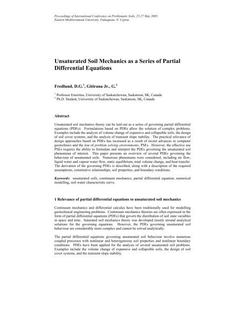
Figure 1 presents the elements required in order to model an unsaturated soil problem,
considering as an example a three-dimensional slope. According to the continuum mechanics
approach, unsaturated soil phenomena can be modelled as follows:
1. Identify the physical processes of concern associated with the problem in hand;
2. Establish the “continuous variables” acting upon a representative elemental volume
(REV) of soil;
3. Develop field equations governing the physical processes of concern by making the
assumption that the media can be considered a continuum from a macroscopic
standpoint (i.e., considering a REV of soil) and using measurable soil properties:
a. Develop conservation laws;
b. Develop constitutive laws;
c. Develop a final system of well-posed determinate partial differential equations.
4. Establish initial, internal, and boundary conditions for the problem;
5. Provide a mathematical solution of the system of PDEs.
The objective of this paper is to show how unsaturated soils theory can be laid out based on
the continuum mechanics approach described above and as a series of PDEs. An overview of
PDE’s governing the behaviour of unsaturated soils is presented along with a detailed
description of how the PDE’s can be derived. Several phenomena are considered herein,
including liquid water flow, water vapour flow, air flow, static equilibrium, total volume
change, and heat flow.
The coupling between several unsaturated soil phenomena are described in terms of the
coefficients and variables of the PDEs. The PDEs describing unsaturated soil behaviour may
also be simplified and de-coupled, in order to neglect processes that are unimportant in certain
situations. Several degrees of de-coupling traditionally adopted in commercially available
software packages are described and the consequences of such simplifications are explored.
The Cartesian coordinate system was adopted throughout the paper and all equations were
written for a general three-dimensional case. Two-dimensional conditions can be easily
obtained, as a simplification of the equations presented herein. The equations presented can
also be converted to axis-symmetric conditions by using a cylindrical coordinate system.
Though tensor notation offers an elegant and general way of presenting the differential
equations governing unsaturated soil behaviour, engineering notation was adopted. Engineers
in general are more prepared to understand the physics of soil behaviour, but may not fully
grasp tensor notation.
2

Fredlund, D.G., Gitirana Jr., G.
Initial conditions (transient problems):
- pore-air pressure, pore-water pressure,
stresses, stress history, temperature, etc.
Internal conditions:
- pore-air, pore-water, and heat sinks
- body forces (gravity)
Boundary conditions:
- pore-water pressure and/or water flow
- pore-air pressure and/or air flow
- displacements and/or external forces
- temperature and/or heat flow
- etc.
Problem
Geometry
dz
O
Representative Elemental
Volume – R.E.V.
y
z
dx
dy
x
Water
table
⎡Distribution of ⎤
⎢
⎥ =
⎣uw,
ua,
σ,
u,
v,
w,
T,
etc. ⎦
∫
∫
VolumeTime
PDE system derived using the R.E.V.
Figure 1
Continuum mechanics approach for solving unsaturated soil problems:
problem domain subjected to initial and boundary conditions and governed by
a system of PDE’s (variables defined later in the text).
2 Assumptions traditionally adopted in the derivation of partial differential
equations governing unsaturated soil behaviour
A series of assumptions form the backdrop for the derivation of the partial differential
equations governing the behaviour of unsaturated soils. The following set of assumptions can
be considered generally valid:
1. soil phases can be described using a continuum mechanics approach;
2. pore-air and all of its constituents (including water vapour) behave as ideal gases;
3. local thermodynamic equilibrium between the liquid water and water vapour phases
exists at all times at any point in the soil; and
4. atmospheric pressure gradients are negligible.
In addition to the above general assumption, a number of specific simplifications can be
adopted. The following simplification limit the generality of the PDE’s presented herein, but
are valid for most conditions found in the practice of geotechnical engineering:
1. liquid water and soil particles are assumed incompressible;
2. small strain theory is valid;
3. thermal strains are negligible;
3

GEOPROB 2005
4. osmotic pressure gradients become negligible at total suctions less than 1500 kPa;
5. temperature within the soil remains below the boiling point and above the freezing
point of water at all times;
6. hysteretic behaviour of the soil-water characteristic curve can be neglected or
approximated by taking the logarithmic average between the main drying and main
wetting curves.
The six assumptions described above may become inadequate under certain situations. For
instance, small strain theory may result in high inaccuracies for highly compressible media,
such as certain landfills and mine tailings. Water compressibility has an important impact on
the analysis of regional groundwater systems (i.e., large domains). Water flow analysis may
require the consideration of freeze and thawing for cold regions. Also, thermal strains may be
of interest in specific design conditions, such as confined clay buffers used for underground
radioactive waste disposal.
Other simplifying assumptions are acceptable for numerous practical problems but are not
adopted herein. Some of these assumptions are as follows:
1. the air phase may be assumed as in permanent contact with the atmosphere (i.e., poreair
pressure gradients are negligible);
2. dissolution of air into the liquid water phase may be neglected;
3. overall volume change may be neglected in air and water flow analyses;
The description of typical assumptions presented in this section is not exhaustive. Additional
assumptions associated with the development of constitutive relationships will be described
along this paper.
3 Stress state variables
Appropriate stress state variables must be used, that are able to accommodate the
characteristics of a multi-phased continuum, such as an unsaturated soil. Fredlund and
Morgenstern (1977) presented a theoretical justification for the use of two independent stress
state variables.
The stress state variables for an unsaturated soil are made of possible combinations of the
total stress, σ, the pore-air pressure, u a , and the pore-water pressure, u w . The net stress, (σ –
u a ), and matric suction, (u a – u w ), are normally used. Tensors for the two independent stress
variables can be written as follows:
⎡σ
⎢
⎢
⎢
⎣
x
τ
− u
τ
yx
zx
a
σ
y
τ
τ
xy
− u
zy
a
τxz
⎤
⎥
τ yz ⎥
σ − ⎥
z ua
⎦
and
⎡u
⎢
⎢
⎢
⎣
a
− u
0
0
w
u
a
0
− u
0
w
u
a
0
0
− u
w
⎤
⎥
⎥
⎥
⎦
(1)
where:
σ i = normal stress acting on the i plane, on the i direction;
τ ij = shear stress acting on the i plane, on the j direction.
The net stress and matric suction tensors reduces to a single stress variable (i.e., effective
stress) for saturated conditions, providing an approach consistent with that traditionally used
in saturated soil mechanics (Terzaghi, 1943). The two stress state variables above are used
throughout this paper.
4

Fredlund, D.G., Gitirana Jr., G.
4 Differential conservation equations for unsaturated soils
Three fundamental conservation laws are generally required in order to establish governing
equation for unsaturated soils; namely, conservation of momentum; conservation of mass; and
conservation of heat. A continuum mechanics framework is employed herein, resulting in the
use of differential calculus to represent these fundamental conservation laws. The assumption
that the variables involved are continuous is assumed valid from a macroscopic,
phenomenological standpoint.
4.1 Conservation of linear and angular momentum
The distribution of total stresses within an unsaturated soil is governed by the static
equilibrium of forces. Stresses acting in each face of a REV can be decomposed as the
normal and shear components in the x, y, and z-directions, as shown in Fig. 2. According to
the convention adopted herein, the stresses shown in Fig. 2 are all positive. The balance of
angular momentum, taken with respect to any axis, shows that the Cauchy tensor (Eq. 1) must
be symmetric (i.e., τ ij = τ ji ). The balance of linear momentum (i.e., the equilibrium of forces)
results in the PDE’s governing static equilibrium of forces (Chou and Pagano, 1992). The
equilibrium equations, in Cartesian coordinates, are as follows:
∂σ
∂x
∂τ
x
xy
∂x
∂τ
∂x
xz
∂τ xy
+
∂y
∂σ y
+
∂y
∂τ yz
+
∂y
∂τ
+
∂z
xz
∂τ yz
+
∂z
∂σ
+
∂z
z
+ F
x
+ F
+ F
y
z
= 0
= 0
= 0
(x-direction)
(y-direction)
(z-direction)
(2)
where:
F i = body force acting on the i direction per unit of volume, kN/m 3 .
τ
yx
∂τ
yx
+ dy
∂y
σ
y
∂σ
y
+
∂y
dy
τ
yz
∂τ
yz
+
∂y
dy
dy
dz
O
y
τ xy
σ x
τ xz
σ z
τ zy
z
F x
F z F y
τ zx
τ yz
τ yx
σ y
x
τ
σ
τ
xz
x
xy
∂τ
xz
+ dx
∂x
∂σ
x
+ dx
∂x
∂τ
xy
+ dx
∂x
dx
Figure 2 Soil representative elemental volume and stresses acting on the REV faces
(stresses at the negative z-face are not shown for clarity).
5

GEOPROB 2005
The same equations above can be obtained by defining an arbitrary finite body and utilizing
the divergence (or Gauss) theorem. It is important to point out that pore-water and pore-air
pressures have no direct role in the equilibrium of forces acting upon the faces of an
unsaturated soil REV. However, the partitioning of total forces into total stresses, pore-water,
and pore-air pressures will depend on the relative compressibility of each soil phase.
4.2 Conservation of mass and heat energy
Differential equations for the conservation of mass of water, mass of air, and heat can be
developed by considering a REV of soil (Fig. 3). The equations of conservation can be
derived by taking the flow rates in and out of the REV and equating the difference to the rate
of change of mass or heat stored in the REV with time. The following differential equations
are obtained by considering three-dimensional flow conditions:
w
w
w
∂q
∂q
x y ∂qz
− − −
∂x
∂y
∂z
a
a
y
1
=
V
0
∂M
∂t
∂q
∂q
x ∂qz
1 ∂M
a
− − − =
∂x
∂y
∂z
V ∂t
h
h
y
∂q
∂q
x ∂qz
1 ∂Qh
− − − =
∂x
∂y
∂z
V ∂t
a
h
0
0
w
(conservation of mass of pore-water) (3)
(conservation of mass of pore-air) (4)
(conservation of heat) (5)
where:
= total water and air flow rate in the i-direction across a unit area of
the soil, kg/m 2 s;
w
q i = ρ w v w i , kg/m 2 s;
a
q i = ρ a v a i , kg/m 2 s;
ρ w = density of water, ≈ 1000.0 kg/m 3 ;
ρ a = density of air, kg/m 3 ;
w, a
v i = water and air flow rate in the i direction across a unit area of the
soil, m/s;
V 0 = referential volume, V 0 = dxdydz, m 3 ;
q i
w, a
y
q
y
∂q
y
+ dy
∂y
∂q
z
q
z
+ dz
∂z
q x
dy
z
q z
∂q
x
q
x
+ dx
∂x
dz
O
dx
q y
x
q x , q y , q z – rate of flow of mass
of air, mass of water, or heat
Figure 3 Soil representative elemental volume and fluxes q at the REV faces.
6

Fredlund, D.G., Gitirana Jr., G.
M w, a = mass of water and air within the representative elemental volume,
kg;
t = time, s;
h
q i heat flow rate in the i direction per unit of total area, J/(m 2 s);
Q h heat within the representative elemental volume, J.
The total water flow rate, v w , also known as specific discharge, is a macroscopic measure of
flow rate through soils. A measure of the average actual flow velocity for a saturated soil can
be obtained by dividing v w by the soil porosity (n = V v /V). The total flow rate, v w , may take
place as liquid water and/or water vapour flow, as will be explained in the next sections. The
average actual air flow velocity for a completely dry soil can be obtained by dividing v a by the
porosity. The total air flow rate, v a , may take place as free air and/or air dissolved in liquid
water, as will be explained in the next sections. Heat flow may take place by conduction,
convection, or latent heat consumption. The mechanisms of air, water, and heat flow within
unsaturated soils will be described in details later in this paper.
5 Strain-displacement relationships and compatibility equations
The classical definition of strain can be applied to an unsaturated soil body. The normal strain
in a given direction, ε, is defined as the unit change in length (change in length per unit
length) of a line which was originally oriented in the given direction. Shear strain, γ, is
defined as the change in the right angle between reference axes, measured in radians (Chou
and Pagano, 1992). The relationships between the normal and shear strains and the
displacement in the x-, y-, and z-direction are as follows:
ε
γ
x
xy
∂u
∂v
∂w
= , ε y = , εz
=
(6)
∂x
∂y
∂z
∂u
∂v
∂u
∂w
∂v
∂w
= + , γ xz = + , γ yz = +
(7)
∂y
∂x
∂z
∂x
∂z
∂y
where:
ε i = normal strain in the i-direction;
γ ij = shear strain with respect to the i and j reference axes;
u, v, w = displacement in the x-, y-, and z-direction, respectively.
The relationships above are obtained by making the assumption of small strains (i.e.,
neglecting the product of two or more derivatives of displacement). The assumption of small
strains adopted herein applies to most engineering problems. Small strain formulations may
be applied to large strain problems if geometry updating is performed along with an
incremental analysis (Cook, 1981).
In addition to the strain-displacement relationships, strain compatibility equations can be
derived (Chou and Pagano, 1992). The geometric significance of the strain compatibility
equations rests in the fact that a strain field that does not satisfy the compatibility equations
may result in “gaps” in the continuum. Nevertheless, compatibility equations are irrelevant
because the continuous displacement functions generally used automatically satisfy the
compatibility equations.
6 Constitutive laws for unsaturated soils
The modelling of unsaturated soil behaviour requires constitutive laws for stress-strain
7

GEOPROB 2005
behaviour, volume change of the pore-air and pore-water phases, and flow of pore-water,
pore-air, and heat. Constitutive laws must be combined with the conservation laws in order to
render the governing equations determinate.
Constitutive laws are generally established based on the phenomenological observation of the
relationships between the state variables. Most constitutive laws for unsaturated soil are
defined based on nonlinear soil properties (i.e., stress state dependent). The term unsaturated
soil property function is used herein to refer to the function describing the relationship
between a soil property and the stress state variables (σ – u a ) and (u a – u w ).
6.1 Stress-strain relationship
Numerous stress-strain relationships have been proposed for unsaturated soils, mostly as
extensions of existing models for saturated soils. Figure 4 presents an overview of some
types of stress-strain relationships available in the literature. The most popular stress-strain
models available can be classified as either elastic or elastoplastic models. Visco-elastoplastic
and other types of models that have not received much attention in unsaturated soils
modelling have not been included in Fig. 4.
Regardless of the model adopted, most elastic and elastoplastic stress-strain relationships for
unsaturated soils can be written in the following generic format:
1
dε = D
− d(
σ − uaδ)
+ Hd(
ua
− uw)
(8)
d( σ − uaδ)
= Ddε
− hd(
ua
− uw)
(9)
where:
d = indicates increment;
ε T = ε ε ε γ γ γ ] ;
[ x y z xy xz yz
Stress-strain models for saturated
and unsaturated soils
Elastic
models
Elastoplastic
models
Linear models
Nonlinear models
E-µ models
K-G models
Isotropic models
Anisotropic models
Generalised Hooke’s law,
State surface,
Stress-induced anisotropy,
Hyperbolic model,
etc.
Perfect plastic
models
Associated flow rules
Non associated flow rules
Tresca, Von Mises,
Mohr-Coulomb,
Druker-Prager,
Spatially Mobilized Plane,
etc.
Hardening
models
Associated flow rules
Non associated flow rules
Isotropic hardening
Kinematic hardening
Cam-Clay,
Modified Cam-Clay,
Barcelona Basic Model,
etc.
Figure 4 Stress-strain constitutive models for saturated and unsaturated soils.
8

Fredlund, D.G., Gitirana Jr., G.
D, H = constitutive matrices;
D =
⎡D11
D21
D31
D41
D51
D
⎢
⎢
D12
D22
D32
D42
D52
D
⎢D13
D23
D33
D43
D53
D
⎢
⎢D14
D24
D34
D44
D54
D
⎢D
⎢
15 D25
D35
D45
D55
D
⎢⎣
D16
D26
D36
D46
D56
D
Η Τ = [ H 1 H 2 H3
H 4 H5
H6]
;
h = DH;
h Τ = h h h h h ] ;
[ 1 2 3 4 5 h6
[ x σ y σz
τxy
τxz
τ yz
[ 1 1 1 0 0 0 .
σ T = σ ] ;
δ T ]
61
62
63
64
65
66
⎤
⎥
⎥
⎥
⎥ ;
⎥
⎥
⎥
⎥⎦
The bold characters indicate matrices and vectors. The superscript ( T ) designates a transposed
matrix. Some matrices were written in the transposed form for convenience.
6.1.1 Elastic models
Elastic models for unsaturated soils (left branch in Fig. 4) are usually based on extensions of
Hooke’s law (Fredlund and Morgenstern, 1976), using the two stress state variables, (σ – u a )
and (u a – u w ):
1
µ
1
dε
x = d(
σx
− ua
) − d(
σ y + σz
− 2ua
) + d(
ua
− uw)
E
E
H
1
µ
1
dε
y = d(
σ y − ua
) − d(
σx
+ σz
− 2ua
) + d(
ua
− uw)
E
E
H
1
µ
1
dε
z = d(
σz
− ua
) − d(
σx
+ σ y − 2ua
) + d(
ua
− uw)
E
E
H
1
1
1
dγ
xy = dτxy
, dγ
xz = dτxz
, and dγ
yz = dτ
yz
G
G
G
(10)
where:
E = Young modulus;
µ = Poisson’s ratio;
H = elastic modulus for soil structure with respect to suction change;
G = shear modulus, G = E 2 (1 − µ ) .
The constitutive matrices D, H, and h corresponding to Eq. (9) can be promptly written.
Some nonlinear strain characteristics can be accounted for by using incremental analysis and
the state surface concept (Matyas and Radakrishna, 1968). Using coefficients of
compressibility obtained from the volume the void radio state surface, the values of E and H
can be obtained for each incremental step as follows:
3 (1 − 2µ
)
E =
s
m1
(11)
3
H =
s
m2
(12)
9

GEOPROB 2005
where:
s
m 1 =
s
m 2 =
dεv
1 de
=
;
d( σmean
− ua
) 1+
e0 d(
σmean
− ua
)
dεv
1 de
=
;
d u − u ) 1+
e d(
u − u )
( a w 0 a w
dε v =
dV ;
V 0
dε s
s
v = m1 d( σmean
− ua
) + m2d( ua
− uw
) ;
σ mean = total mean stress, σ mean = (σ x + σ y + σ z )/3;
e 0 = initial void ratio;
e = state surface for void ratio, e = f(σ mean – u a , u a – u w ).
Equations (11) and (12) are based on the assumption that the volume change of unsaturated
soils is a function of changes in net mean stress and soil suction. Equation (11) alone does
not provide a way of computing µ. The value of Poisson’s ratio must be estimated or
obtained from other means. For instance, µ can be obtained through triaxial or oedometric
tests with measurement of lateral strains of lateral stresses, respectively.
The stress-induced anisotropy notably found in highly collapsible soils can be considered by
using a stress-dependent Poisson’s ratio and anisotropy coefficients applied to the H i modulus
(Pereira and Fredlund, 2000). Shear strength can be addressed by using a hyperbolic curve
(Duncan and Chang, 1970) for the unsaturated soil Young modulus near failure. Elastic
models can be considered generally appropriate for the analysis of monotonic net stress and
suction paths. However, elastic models may not be accurate when non-monotonic paths take
place because the distinction between recoverable and irrecoverable strains is not considered.
6.1.2 Elastoplastic models
Elastoplastic models (right main branch in Fig. 4) may be employed in order to address
features of soil behaviour such as yield and irrecoverable strains. Most elastoplastic models
found in the literature are generally based on the same fundamental principles, but use
different yield criteria, flow rules, and compressibility functions. Figure 4 lists several yield
criteria used by perfect plastic models. Perfect plastic formulations for saturated soils can be
extended to unsaturated soils by using the generalised Hooke’s law and by incorporating the
effect of soil suction into the yield criterion (Pereira, 1996).
Yield surfaces can be combined with hardening rules and cap surfaces. Hardening rules are
used in order to reproduce changes in the size of the yield surface (isotropic hardening) or
shifts in the yield surface position (kinematic hardening). Cap surfaces are used in order to
account for yield that occurs at stress states below failure conditions.
Numerous models have been proposed for unsaturated soils based on a critical state
framework. Some of the early model were proposed by Karube and Kato (1989), Alonso et
al. (1990), Wheeler and Sivakumar (1995), and Cui and Delage (1996), amongst others.
Great emphasis has been given to soils compacted at collapsible conditions. Most models are
based on isotropic hardening laws and on yield surfaces that expand for increasing soil
suctions. Collapse is reproduced by using appropriate modes of expansion of the yield curves
and appropriate variations in soil compressibility for different suctions. Research continues to
be undertaken in order to refine elastoplastic models for unsaturated soils.
Lloret and Ledesma (1993) present the manner how the elastoplastic stress-strain relationship
can be written for unsaturated soils. The yield functions and corresponding flow rules
10

Fredlund, D.G., Gitirana Jr., G.
proposed by Alonso et al. (1990) were considered. The general stress-strain relationship takes
the following form:
⎪⎧
if F1
≤ 0 and F2
≤ 0
⎨
⎪⎩ if F1
> 0 or F2
> 0
e e
d(
σ − uaδ)
= D dε
− h d(
ua
− uw)
ep ep
d(
σ − uaδ)
= D dε
− h d(
ua
− uw)
(13)
where:
F 1 =
yield function for load or suction decrease,
F 1 = f(σ – u a , u a – u w , Γ);
F 2 =
yield function for suction increase,
F 2 = f(σ – u a , u a – u w , Γ);
D e , H e = elastic constitutive matrices, defined according to Eq. (10);
D ep , H ep = elastoplastic constitutive matrices;
D ep =
T
e 1 e ∂G1 ⎛ ∂F
e
D D
D
A Acr
ua
u ⎟ ⎞
⎜ 1
−
;
− ∂(
σ − )
⎝ ∂(
σ − a ) ⎠
e
D Hs
+
h ep = ⎡
T
⎛ F1
F
⎤
⎢
∂ ⎞
∂ 1 1 ∂G
;
⎜ ⎟ e
⎥
e 1
−
⎢
( ua
)
D Hs
+
D
∂(
u a−uw)
⎥ A − Acr
∂(
σ − ua
)
⎣
⎝ ∂ σ − ⎠
⎦
H s =
⎪⎧
e
if F2
≤ 0 H
⎨
;
e ep
⎪⎩ if F2
> 0 H + H
A =
T
∂F1
⎛ ∂Γ ⎞ ∂G1
− ⎜ ⎟ ;
∂Γ
p
⎝ ∂ε ⎠ ∂(
σ − u )
A cr =
⎛ ∂F1
⎞ e ∂G1
− ⎜ ⎟
D
( ua
)
;
⎝ ∂ σ − ⎠ ∂(
σ − ua
)
G 1 = flow rule, G 1 = f(σ – u a , u a – u w , Γ);
Γ = hardening parameter;
T
⎛ ∂F
⎞
⎜ ⎟
u ⎝ ∂(
σ − a ) ⎠
T
1
= [ ∂F1
∂F1
∂F1
∂F1
∂F1
∂F
1 ] ;
∂(
σ − u ) ∂(
σ − u ) ∂(
σ − u ) ∂τ ∂τ ∂τ
T
⎛ ∂G
⎞
⎜ ⎟
u ⎝ ∂(
σ − a ) ⎠
x
a
y
a
1
= [ ∂G1
∂G1
∂G1
∂G1
∂G1
∂G
1 ] .
∂(
σ − u ) ∂(
σ − u ) ∂(
σ − u ) ∂τ ∂τ ∂τ
x
a
y
a
a
z
z
a
a
xy
xy
xz
xz
yz
yz
The term Γ is generally taken as equal to the pre-consolidation stress for saturated conditions.
Different functions for F 1 , F 2 , G 1 , G 2 and for the soil compressibility are defined by each
model found in the literature. The original references should be consulted for further details.
Equations (8) and (9) can be used to provide generic equations to be used in the derivation of
the partial differential equations governing unsaturated soil behaviour. Nevertheless, Eq. (10)
will be employed herein for the derivation of the governing PDE’s. The selection of Eq. (10)
was based on its simplicity and straightforward relation with the soil compressibility
coefficients.
6.2 Shear strength
Shear strength characteristics may be incorporated into the PDE’s governing unsaturated soil
behaviour through modification to the D, H, and h matrices. For instance, shear strength is
used by the Hyperbolic-type models to control the shape of the Young modulus function
11

GEOPROB 2005
(Duncan and Chang, 1970). The shear strength equations can also be used to define the yield
criteria used by elastoplastic models.
Several shear strength equations were listed in Fig. 4, such as the Tresca, Von Mises, and
Mohr-Coulomb equations. Extensions of the Mohr-Coulomb criterion for saturated soils are
widely used to represent the shear strength for an unsaturated soil, τ ff . Fredlund et al. (1996)
proposed the following equation based on the Mohr-Coulomb criterion:
τ
ff
κ
= c ' + ( σ − u ) tan φ ' + ( u − u ) Θ tan φ'
(14)
n
a
f
a
w
where:
τ ff = shear stress at failure, acting on the failure plane;
(σ n – u a ) f = net normal stress acting on the failure plane;
c’ = cohesion;
φ’ = friction angle;
Θ =
dimensionless parameter to account for the wetter area of
contact;
κ =
fitting parameter to account for any non-linearity between
the area and volume representation of the amount of water
contributing to the shear strength.
The shear strength for an unsaturated soil can be predicted using the soil-water characteristic
curve and the saturated shear strength parameters, c’ and φ’. According to Fredlund et al.
(1996), Θ can be assumed as equal to the degree of saturation, S. Experimental evidence
shows that the slope of the plot of shear strength versus soil suction begins to deviate from the
effective angle of internal friction as the soil desaturates. This reduced slope is associated
with the reduction in the wetted area of contact past the air-entry value.
Vanapalli et al. (1996) presents a slightly modified procedure, defining
Θ = Θn
= ( S − Sres
) ( 1 − Sres
) and making κ = 1. This second procedure, based on
normalised (or effective) water content, renders the envelope potentially less flexible if the
fitting parameter κ is not used.
6.3 Water phase volume change
The constitutive relationship for the amount of water store in the soil pores is usually given in
terms of volume of water. Water compressibility is generally neglected. The change in
volume of water stored in the soil pores can be written as function of elastic coefficients of
compressibility, m 1 w and m 2 w , or volumetric modulus, E w and H w , as follows:
dV
V
0
w
= m
w
1
3
=
E
w
d
w
( σ − u ) + m d( u − u )
d
mean
( σ − u ) + d( u − u )
mean
a
a
2
1
H
w
a
a
w
w
(15)
where:
w
m 1 =
S de e dS
+
;
1+
e0 d(
σmean
− ua
) 1+
e0
d(
σmean
− ua
)
w
m 2 =
S de e dS
+
;
1+
e0 d(
ua
− uw)
1+
e0
d(
ua
− uw)
S = degree of saturation, S = f(σ mean – u a , u a – u w );
12

Fredlund, D.G., Gitirana Jr., G.
e = void ratio, e = f(σ mean – u a , u a – u w );
E w =
w
3 m 1 ;
H w =
w
1 m 2 .
Equation (15) is based on the assumption that changes in the volume of pore-water stored in
the soil are a function of changes in net mean stress and soil suction and are independent of
changes in shear stresses. The use of state surfaces for void ratio and degree of saturation
provides an effective method for computing E w and H w . Hysteretic characteristics of the porewater
storage can be addressed using more sophisticated relationships. However, the simple
elastic relationships based on state surfaces can adequately reproduce monotonic stress paths.
Coupled PDE systems are often written in terms of displacements and pore pressures.
Changes in (σ mean – u a ) present in Eq. (15) can be written in terms of changes in (u a – u w ) and
strains using Eq. (10), as follows:
dV
V
0
w
w
1
w
2
= β dε
+ β d(
u − u )
(16)
v
a
w
where:
w
β 1 =
w
β 2 =
m
m
w
1
s
1
m
w
2
=
E
m
−
w
w s
1 m2
s
m1
E
;
(1 − 2µ
)
1
=
H
w
3
−
E
w
E
.
H (1 − 2µ
)
Equation (16) results in a smooth transition between saturated and unsaturated conditions,
provided that appropriate constitutive coefficients are employed. As the soil saturates the
s s w w
effects of changes in soil suction and net stresses become equal (i.e., m1 = m2
= m1
= m2
).
Consequently, Eq. (16) shows that for saturated conditions water volume changes are equal to
changes in void ratio.
6.4 Air phase volume change
The characterisation of the air phase volume change requires the determination of two of the
following variables; namely, V a , M a , and ρ a . The air phase is highly compressible, and its
density is given by the following equation:
M W
ρ
a
a = = ua
(17)
V RT
a
a
where:
ρ a = density of the bulk air phase, kg/m 3 ;
W a = molecular weight of pore-air, 28.966 kg/kmol;
u a
= total pressure in the bulk air phase, u a +u atm , kPa;
u a = pore-air pressure, kPa;
u atm = atmospheric pressure, 101.325 kPa;
Three volume change measurements can be made for an unsaturated soil; namely, overall,
pore-water, and pore-air volume change. The combination of any two of these three volume
change measurements provides a complete description of volume change within an
13

GEOPROB 2005
unsaturated soil. Pore-air volume changes have proven more difficult to measure than those
of the pore-water phase. Therefore, it has become common practice to measure overall and
pore-water volume changes. The volume of pore-air may be computed as follows:
Va
V0
Vv
Vw
= − (1 − H c )
Vo
Vo
= n(1
− S + H cS)
(18)
where:
H c = Henry’s volumetric coefficient of solubility, V ad /V w ;
V ad = volume of air dissolved in the pore-water.
H c is also known as the volumetric coefficient of solubility. At a constant temperature, the
volume of dissolved air is a constant for different pressures. Dorsey (1940) cited by Fredlund
and Rahadjo (1993) presents values of H c for various temperatures. The density of air is
assumed as being the same for the free air and for dissolved air.
The volume change constitutive relationship for the water phase can be obtained by taking an
incremental form of Eq. (18) and using the constitutive relationship for pore-water volume
change, described by Eq. (16):
dV
V
0
a
a
1
a
2
= β dε
+ β d(
u − u )
(19)
v
a
w
where:
a
1
w
1 1 c
β = − β (1 − H ) ;
a
2
w
2 c
β = − β (1 − H ) .
Equation (19) shows how the volume change characteristics of the air phase can be directly
obtained from the volume change characteristics of the water phase and soil skeleton.
6.5 Flow laws
Table 1 presents an overview of flow laws traditionally used for modelling unsaturated soil
flow behaviour. The flow laws establish relationships between measures of flow and driving
potentials. Driving potentials can be established based on spatial gradients of the energy
stored per unit volume (Bear, 1972). The several flow equations have the same format, but
distinct potentials and properties. The flow laws presented in Table 1 are well established
equations that have been experimentally verified.
Pore-air and pore-water have both miscible and immiscible mixture characteristics. Pore-air
can flow as free air, as dissolved air diffusing through the liquid water, or as dissolved air
carried by the liquid water. Pore-water can flow as liquid water, as water vapour diffusing
through the free air-phase, or as water vapour carried by moving free air-phase. Some flow
mechanisms are essential in the modelling of certain air and water flow conditions. For
instance, evaporation cannot be properly reproduced without consideration of the water
vapour flow (Wilson et al., 1994). Similarly, the air flow that takes place through saturated
high air-entry value ceramics cannot be understood without consideration of the movement of
dissolved air through the liquid water phase (Fredlund and Rahardjo, 1993).
14

Fredlund, D.G., Gitirana Jr., G.
Table 1 – Overview of types of flow within an unsaturated soil and the corresponding
mechanisms, driving potentials, and flow laws.
Type of flow
(1)
Flow mechanism
(2)
Driving Potential
(3)
Flow Law
(4)
Liquid water,
wl
v Hydraulic head, h (m) Darcy’s law
Flow of
w
water, v
Water vapour diffusion,
vd
v
Mass concentration of vapour per
unit volume of soil, C v (kg/m 3 )
Modified
Fick’s law
Water vapour carried by
va
bulk air flow, v
Mass concentration of air per unit
volume of soil, C a (kg/m 3 )
Modified
Fick’s law
Interphase
liquidvapour
flow
Thermodynamic
equilibrium
--- (*)
Lord Kelvin’s
equation
Free air,
af
v
Mass concentration of air per unit
volume of soil, C a (kg/m 3 )
Modified
Fick’s law
Flow of air,
a
v
Dissolved air diffusion,
ad
v
Mass concentration of dissolved air
per unit volume of soil, C ad (kg/m 3 )
Modified
Fick’s law
Dissolved air carried by
aa
liquid water flow, v
Hydraulic head, h (m)
Darcy’s law
Flow of
h
heat, q
Heat by conduction,
c
q Temperature, T (ºC) Fourier’s law
Latent heat --- (*)
Interphase
liquid-vapour
flow
(*) local thermodynamic equilibrium assumed; function of the rate of vapour flow.
The following sections present a concise description of the flow laws listed in Table 1. All
flow equations presented in this section were written for the y-direction (i.e., the direction
corresponding to elevation) and considering isotropic conditions. Similar equations can be
written for the x- and z-directions by using the appropriate gradient directions. Anisotropy
can be easily incorporated into the flow equations by using conductivity ellipsoids. These
ellipsoids can be defined by an anisotropy ratio and by the direction of “principal
conductivities”, as shown by Bear (1972) and Freeze and Cherry (1979).
6.5.1 Flow of liquid water
The flow rate of liquid water in saturated/unsaturated soils can be described by using a
generalisation of Darcy’s Law (Bear, 1972), where the driving mechanism is the total head
gradient and the hydraulic conductivity varies with matric suction, (u a – u w ). The generalised
Darcy’s law can be written as follows:
v
wl
y
w ∂h
= −k
(20)
∂y
where:
v y
wl
= liquid pore-water flow rate in the y-direction across a unit area
of the soil due to hydraulic head gradients, m/s;
15

GEOPROB 2005
k w = hydraulic conductivity, k w = f(u a – u w ), m/s;
h = hydraulic head, m;
h =
u + y
γw
;
u w = pore-water pressure, kPa;
γ w = unit weight of water, ≈ 9.81 kN/m 3 ;
y = elevation, m.
The hydraulic conductivity function (i.e., the function giving the value of k w for any value of
(u a – u w ) may be obtained experimentally using laboratory or field tests, or estimated using the
saturated hydraulic conductivity and the soil-water characteristic curve (Fredlund et al.,
1994). The use of a continuous k w function provides a smooth transition between the
saturated and unsaturated condition.
6.5.2 Flow of water vapour
Water vapour flow through soils takes place by two mechanisms. Pore-water vapour may
flow independently from the pore-air phase, driven by gradients in vapour concentration.
Water vapour flow driven by vapour concentration may take place even if the bulk pore-air is
at rest. Pore-water vapour may also be carried by the bulk pore-air phase, which may flow
driven by gradients in the total pore-air pressure. The sum of these two vapour flow
components results in the total water vapour flow, v v .
The flow rate of water vapour due to gradients in vapour concentration may be described by a
modified form of Fick’s law (Philip and de Vries, 1957 and Dakshanamurthy and Fredlund,
1981):
v
vd
y
D
= −
ρ
w
v
D
= −
ρ
v
w
∂C
∂y
v
∂C
∂p
v
v
∂pv
∂y
D
= −
ρ
v*
w
∂pv
∂y
(21)
where:
= pore-water vapour flow rate in the y-direction across a unit area
of the soil due to vapour concentration gradients, m/s;
D v = molecular diffusivity of vapour through soil, m 2 /s;
ρ w = density of water, ≈ 1000.0 kg/m 3 ;
C v = concentration of water vapour in terms of the mass of vapour
per unit volume of soil, C v = ρ v (1 – S)n, kg/m 3 ;
ρ v = density of the water vapour, ρ v = W v p v /(RT), kg/m 3 ;
W v = molecular weight of water vapour, 18.016 kg/kmol;
p v = partial pressure of water vapour, kPa;
R = universal gas constant, 8.314 J/(mol.K);
T = temperature, K;
S = degree of saturation, S = V w /V v ;
n = porosity, n = V v /V 0 ;
V w , V v = volume of water and voids in the elemental volume,
respectively, m 3 ;
D v* = (1 – S)nD v W v / RT, (kg.m)/(kN.s).
v y
vd
The soil properties D v and D v* can be directly measured or reasonably estimated by using the
value of molecular diffusivity of vapour through air (0.229×10 -4 (1+T/273.15) 1.75 m 2 /s,
Kimball et al., 1976 cited by Wilson et al., 1994) and combining that value with a tortuosity
16

Fredlund, D.G., Gitirana Jr., G.
factor. Ebrahimi-B et al. (2004) presents a summary of tortuosity coefficient functions
proposed in the literature and shows that most existing functions result in similar values for
the ranges of soil suction were vapour flow predominates over liquid flow.
The flow rate of water vapour due to bulk pore-air flow may also be described by a modified
form of Fick’s law (Philip and de Vries, 1957 and Dakshanamurthy and Fredlund, 1981).
Using the fraction ρ v /ρ a in order to obtain the fraction of water vapour present in the pore-air,
the following equation can be written:
va ρv
v y = −
ρa
ρv
= −
ρa
a
D
ρw
a
D
ρw
∂Ca
∂y
∂Ca
∂ua
∂ua
∂y
ρv
= −
ρa
a*
D ∂ua
ρw
∂y
(22)
where:
= pore-water vapour flow rate in the y-direction across a unit area
of the soil due to bulk air-phase flow, m/s;
ρ a = density of the bulk air phase, ρ a = W a u
a
/(RT) , kg/m 3 ;
D a = coefficient of transmission of air, m 2 /s;
C a = concentration of air in terms of the mass of vapour per unit
volume of soil, C a = ρ a (1 – S)n;
D a* = (1 – S)nD a W a / RT, (kg.m)/(kN.s).
v y
va
The soil properties D a and D a* can be directly measured or estimated using the same approach
that was described above for D v and D v* . The total flow of water vapour is obtained by
summing v y vd and v y va , given by Eqs. (22) and (23). Taking the sum of the two vapour flow
components and neglecting gradients of atmospheric pressure, the following equation is
obtained:
v
v
y
= v
vd
y
+ v
va
y
D
= −
ρ
v*
w
∂pv
ρ
−
∂y
ρ
v
a
D
ρ
a*
w
∂ua
∂y
(23)
6.5.3 Mass transfer between liquid pore-water and pore-water vapour
Local thermodynamic equilibrium can be assumed between liquid pore-water and pore-water
vapour at any time and at any point in the soil. This assumption means that a change in any
of the state variables; namely, partial vapour pressure, p v , temperature, T, or the total potential
of the liquid pore-water, ψ, results in an immediate change of the other state variables towards
equilibrium of the liquid-vapour system. The assumption of local thermodynamic equilibrium
provides a way of quantifying mass transfer between liquid and vapour water. The following
relationship between p v , ψ, and T can be derived by assuming local thermodynamic
equilibrium (Edlefsen and Anderson, 1943):
p = p
v
−ψWv
ρ wR( T +273.15)
vsate
(24)
where:
p vsat = saturation vapour pressure of the soil water at temperature T, kPa;
ψ = total suction, kPa;
W v = molecular weight of water, 18.016 kg/kmol;
17

GEOPROB 2005
ρ w = water density, ≈ 1000 kg/m 3 ;
R = universal gas constant, 8.314 J/(mol.K);
T = temperature, o C.
Values of saturation vapour pressure, p vsat , are well established and depend primarily on the
vapour temperature (i.e., the vaporization curve). Equation (24) shows that the partial vapour
pressure is equal to the saturation vapour pressure when ψ = 0 kPa and zero when ψ ≈ 1×10 6
kPa. Changes in p v due to changes in ψ at any given fixed temperature are negligible when ψ
< 1500 kPa. As a result, the use of SWCC’s formed by combining matric and total suction
values (Fredlund, 2002) does not affect the value of p v computed using Eq. (24).
It will be shown in the next sections that it is convenient to replace the gradients of p v in Eq.
(23) by gradients of suction, ψ, and temperature, T. A relationship between the gradients of
p v and the gradients of the other two variables, ψ and T, can be determined by deriving Eq.
(24) using the chain rule:
∂pv
∂y
Wv
pv
⎛ ψ ∂T
∂ψ ⎞
=
⎜
−
⎟
ρwR(
T + 273.15) ⎝ ( T + 273.15) ∂y
∂y
⎠
(25)
Soil-water characteristic curve data is generally plotted combining matric suction values up to
1500 kPa and total suction values beyond this value. In order to make Eqs. (24) and (25)
consistent with the “hybrid” SWCC plot, the water potential, ψ, in Eqs. (24) and (25) can be
assumed as equal to the soil suction obtained from the SWCC. Therefore, the term ψ
corresponds to the total suction when values of ψ are larger than 1500 kPa and to matric
suction when values of ψ are lower than 1500 kPa. Assuming that the effect of pore-air
pressure changes is negligible in the computation of vapour pressures, and replacing the term
ψ by -u w , Eq. (25) can be re-written as follows:
∂pv
∂y
Wv
pv
⎛ ∂u
=
⎜
w
ρwR(
T + 273.15) ⎝ ∂y
uw
∂T
⎞
−
⎟
( T + 273.15) ∂y
⎠
(26)
The following equation is obtained by substituting Eq. (26) into Eq. (23):
v
v
y
= v
vd
y
+ v
va
y
k
= −
γ
vd
w
vd
∂uw
k
+
∂y
γ
w
uw
∂T
k
−
( T + 273.15) ∂y
γ
va
a
∂ua
∂y
(27)
where:
k vd =
k vd =
k va =
k va =
pore-water vapour conductivity by vapour diffusion within the air
phase;
v*
Wv
pv
D
γw
, m/s;
ρwR(
T + 273.15) ρw
pore-water vapour conductivity by advection within the free
pore-air;
γ
a
ρ
ρ
v
a
D
ρ
a*
w
, m/s;
γ w = unit weight of water, kN/m 3 ;
γ a = unit weight of air, kN/m 3 .
18

Fredlund, D.G., Gitirana Jr., G.
6.5.4 Flow of dry air
Pore-air flow takes place primarily by two mechanisms. Pore-air may flow as free air driven
by gradients in its concentration. Pore-air may also flow within the liquid pore-water, as
dissolved pore-air. Dissolved pore-air may be carried by water flow (i.e., advection) or may
flow by pore-air diffusion, driven by gradients in dissolved pore-air concentration.
The mass flux of free pore-air may be described by a modified form of Fick’s law:
af
vy
a
D
= −
ρa
a
D
= −
ρa
∂Ca
∂y
∂Ca
∂ua
∂ua
∂y
a*
D ∂ua
= −
ρa
∂y
(28)
where:
= pore-air flow rate in the y-direction across a unit area of the soil
due to pore-air concentration gradients, m/s;
D a = coefficient of transmission of air, m 2 /s;
ρ a = density of the bulk air phase, ρ a = W a u a /(RT) , kg/m 3 ;
C a = concentration of air in terms of the mass of vapour per unit
volume of soil, C a = ρ a (1 – S)n;
D a* = (1 – S)nD a W a / RT, (kg.m)/(kN.s).
v y
va
All variables and soil properties presented in Eq. (28) have been defined previously. The soil
properties D a and D a* can be directly measured or estimated using the same approach that was
described above for D v and D v* , using a tortuosity coefficient.
The flow of dissolved pore-air driven by gradients in dissolved pore-air concentration may be
described by a modified form of Fick’s law:
ad
v y
ad
D
= −
ρa
ad
D
= −
ρa
∂Cad
∂y
∂Cad
∂ua
∂ua
∂y
ad*
D ∂ua
= −
ρa
∂y
(29)
where:
= dissolved pore-air flow rate of in the y-direction across a unit
area of the soil due to pore-air concentration gradients, m/s.
D ad = molecular diffusivity of dissolved air through water, m 2 /s;
C ad = concentration of dissolved air in terms of the mass per unit
volume of soil, C ad = ρ a SnH c ;
D ad* = nSH
ad
D W RT , (kg.m)/(kN.s).
v y
ad
c
a
The values of D ad* can be directly measured or estimated. Values of D ad and H c found in the
literature are summarised by Fredlund and Rahardjo (1993). As the soil desaturates, the
diffusion of dissolved air through the liquid pore-water decreases and becomes insignificant
when compared with the flow of free pore-air. The decrease in v ad due to desaturation can be
incorporated into the prediction of D ad* by using a tortuosity coefficient.
The flow of dissolved pore-air carried by water flow (i.e., advection) may be described by
19

GEOPROB 2005
Darcy’s law and taking the amount of dissolved air:
aa w ∂h
v y = − Hck
(30)
∂y
where:
v y
aa
= flow rate of dissolved pore-air in the y-direction across a unit
area of the soil due to bulk pore-liquid water flow, m/s.
The total flow of pore-air is obtained by summing the three flow mechanisms, given by Eqs.
(28), (29), and (30):
v
a
y
a
ad
af ad aa k ∂ua
k ∂ua
w ∂h
= vy
+ v y + v y = − − − Hck
(31)
γ ∂y
γ ∂y
∂y
a
a
where:
k a = pore-air conductivity;
k a =
a*
D
γa
ρa
, m/s;
k ad = pore-air conductivity by diffusion within the pore-liquid water;
k ad =
γ
ad
D *
a
ua
, m/s;
γ a = unit weight of air, kN/m 3 .
Equation (31) provides a smooth transition between unsaturated and saturated conditions. As
suction decreases, the soil saturates and k a decreases, eventually reaching zero, for the
saturated condition. However, the flow or air does not cease for saturated conditions. The
pore-air conductivity by diffusion within the pore-liquid water and the flow of dissolved air
carried by bulk liquid-water flow increase for increasing saturation.
6.5.5 Flow of heat by conduction
Heat transfer in soils occurs by three primary mechanisms, namely: conduction; convection;
and latent heat due to phase change. Heat transfer by convection of the pore-fluid in soils is
considerably smaller than conductive heat transfer (Milly, 1984) and is generally neglected.
Changes of phase can take place as vaporization/condensation. Freeze and thawing are of
concern in some unsaturated soil mechanics problems, but are omitted herein.
The conductive heat flow, q i c , can be written as a function of the thermal conductivity of the
soil and the temperature gradient, as follows:
T
q c ∂
y = − λ
(32)
∂y
where:
q y
c
= heat flow rate in the y-direction across a unit area of the soil
due to heat conduction, J/s;
T = temperature, o C;
λ = thermal conductivity, λ = f(u a − u w ), J/(m s o C).
The latent heat flow can be obtained by multiplying the latent heat of vaporization and
condensation, L V , by the amount of vapour flow, given by Eq. (27).
20

Fredlund, D.G., Gitirana Jr., G.
7 Partial differential equations for stress-deformation analysis
Partial differential equations for stress-deformation analysis are required for determining
stress and strain distributions within an unsaturated soil. The stress distribution can be used
for stability analysis and the strain distributions are used in settlement analysis.
The PDEs for stress-deformation analysis can be written by combining the differential
equations governing force equilibrium, Eq. (2), the stress-strain constitutive relationship, and
the relationship between strains and small displacements, Eqs. (6) and (7). The type of stressstrain
relationship adopted determines by a large extent how complex the PDEs for stressstrain
analysis are. It was shown in the previous section that one of the most simple equations
that can be used is based on a generalization of Hooke’s law considering two stress state
variables. Using Hooke’s generalised stress-strain law, Eq. (10), the following PDEs are
obtained:
∂ ⎡ ∂u
∂v
∂w
⎤
⎢σx0
+ D11
+ D12
+ D12
− hd( ua
− uw
) + dua
⎥
∂x
⎣ ∂x
∂y
∂z
⎦
(x-direction) (33)
∂ ⎡ ⎛ ∂u
∂v
⎞⎤
∂ ⎡ ⎛ ∂u
∂w
⎞⎤
+ ⎢τxy0
+ D44
⎜ +
⎟⎥
+ ⎢τxz0
+ D44⎜
+ ⎟⎥
= 0
∂y
⎢⎣
⎝ ∂y
∂x
⎠⎥⎦
∂z
⎣ ⎝ ∂z
∂x
⎠⎦
∂ ⎡ ⎛ ∂u
∂v
⎞⎤
∂ ⎡ ∂u
∂v
∂w
⎢τxy0
+ D44
⎜ +
⎟⎥
+ ⎢σ
y0
+ D12
+ D11
+ D12
∂x
⎢⎣
⎝ ∂y
∂x
⎠⎥⎦
∂y
⎣ ∂x
∂y
∂z
(y-direction) (34)
∂ ⎡ ⎛ ∂v
∂w
⎞⎤
− hd( ua
− uw
) + dua
] + ⎢τ
yz0
+ D44
⎜ +
⎟⎥
+ γ nat = 0
∂z
⎢⎣
⎝ ∂z
∂y
⎠⎥⎦
∂ ⎡ ⎛ ∂u
∂w
⎞⎤
∂ ⎡ ⎛ ∂v
∂w
⎞⎤
⎢τxz0
+ D44⎜
+ ⎟⎥
+ ⎢τ
yz0
+ D44
⎜ +
⎟⎥
∂x
⎣ ⎝ ∂z
∂x
⎠⎦
∂y
⎢⎣
⎝ ∂z
∂y
⎠⎥⎦
∂ ⎡ ∂u
∂v
∂w
+ ⎢σz0
+ D12
+ D12
+ D11
− hd
∂z
⎣ ∂x
∂y
∂z
⎤
a ⎥
⎦
( u − u ) + du = 0
a
w
(z-direction) (35)
where:
σ i0 , τ ij0 = initial stresses;
D 11 = E ( 1− µ ) [(1 + µ )(1 − 2µ
)] ;
D 12 = E µ [( 1+ µ )(1 − 2µ
)] ;
D 44 = E [ 2(1 + µ )] ;
h = E [ H (1 − 2µ
)] ;
γ nat = body force acting downward;
γ nat = γ s ( 1−
n)
+ γ wnS
, kN/m 3 ;
γ s = specific weight of soil particles, kN/m 3 .
The unit weight of the soil, γ nat , shown in Eq. (34) corresponds to the vertical body force. The
initial stresses and pore pressures presented in Eqs. (33) – (35) can be removed in case an
incremental transient approach is considered (i.e., taking derivatives with respect to time of u,
v, w, u w , and u a ). The unsaturated soil properties present in Eqs. (33) – (35) vary with soil
suction and net stresses, and therefore, the PDE is physically non-linear.
Equations (33) – (35) show that the equilibrium of forces within a R.E.V. can be expressed as
a function of the five primary variables; namely, the displacements in the x-, y-, and z-
direction (i.e., u, v, and w), the pore-water pressure, u w , and the pore-air pressure, u a .
21

GEOPROB 2005
Therefore, two additional equations are required in order to render the system of equations
solvable.
The choice of primary variables (i.e., u, v, w, u w , and u a ) is not arbitrary. These five primary
variables result in meaningful boundary conditions. The integration by parts of the secondorder
derivatives from Eqs. (33) – (35) is usually required for their solution. This integration
results in a surface integral that corresponds to a natural (or Neumann) boundary condition.
The natural boundary condition associated with Eqs. (33) – (35) corresponds to external loads
(i.e., forces) in the x-, y-, and z-direction, respectively. Another type of boundary condition
that can be applied to Eqs. (33) – (35) corresponds to pre-determined displacement values
(i.e., essential or Dirichlet boundary conditions). Meaningful essential boundary conditions
could not be established in terms of total stresses. Therefore, the use of u, v, and w as primary
variables is justified.
The three-dimensional equilibrium of forces results in three differential equations. Each
equation is formed by three main partial derivatives of the stress tensor components with
respect to the x, y, and z-directions. The presence of these partial derivatives is a result of the
assumption that the forces and stresses acting on the R.E.V. shown in Fig. 2 are continuously
distributed in space. Because forces and stresses acting on a R.E.V. are assumed to be
continuous variables in space, the spatial distribution of such variables can be described by
the partial derivative of each force of stress component for a given direction.
The various terms within each of the main partial derivatives are a function of the constitutive
law adopted to describe the stress-strain behaviour of the saturated/unsaturated soil. The
PDEs governing equilibrium of forces acting on an unsaturated soil R.E.V. become more
complex when more sophisticated stress-strain models are introduced. However, the general
format of the governing PDEs remains in accordance with Eqs. (33) – (35).
Equations (33) – (35) result in a smooth transition between saturated and unsaturated
conditions, provided that appropriate soil properties are employed. When (u a – u w ) is
positive, the soil behaviour is dictated by the two independent stress state variables for
unsaturated soils and dictated by distinct soil properties associated with each stress state
variables, D ii and h. As the soil saturates and (u a – u w ) approaches zero, m 1 s and m 2 s become
equal to the coefficient of volume change for the soil at a saturated condition (i.e., m v ) and h
becomes 1. Therefore, the PDEs for saturated conditions (i.e., h = 1) are a special case of the
general equations, Eqs. (33) – (35), and can be written as follows:
∂ ⎡ ∂u
∂v
∂w
⎤
⎢σx0
+ D11
+ D12
+ D12
+ duw
⎥
∂x
⎣ ∂x
∂y
∂z
⎦
∂ ⎡ ⎛ ∂u
∂v
⎞⎤
∂ ⎡ ⎛ ∂u
∂w
⎞⎤
+ ⎢τxy0
+ D44
⎜ +
⎟⎥
+ ⎢τxz0
+ D44⎜
+ ⎟⎥
= 0
∂y
⎢⎣
⎝ ∂y
∂x
⎠⎥⎦
∂z
⎣ ⎝ ∂z
∂x
⎠⎦
∂ ⎡ ⎛ ∂u
∂v
⎞⎤
∂ ⎡ ∂u
∂v
⎢τxy0
+ D44
⎜ +
⎟⎥
+ ⎢σ
y0
+ D12
+ D11
∂x
⎢⎣
⎝ ∂y
∂x
⎠⎥⎦
∂y
⎣ ∂x
∂y
∂w
⎤ ∂ ⎡ ⎛ ∂v
∂w
⎞⎤
+ D12
+ duw
⎥ + ⎢τ
yz0
+ D44
⎜ +
⎟⎥
+ γ nat = 0
∂z
⎦ ∂z
⎢⎣
⎝ ∂z
∂y
⎠⎥⎦
∂ ⎡ ⎛ ∂u
∂w
⎞⎤
∂ ⎡ ⎛ ∂v
∂w
⎞⎤
⎢τxz0
+ D44⎜
+ ⎟⎥
+ ⎢τ
yz0
+ D44
⎜ +
⎟⎥
∂x
⎣ ⎝ ∂z
∂x
⎠⎦
∂y
⎢⎣
⎝ ∂z
∂y
⎠⎥⎦
∂ ⎡ ∂u
∂v
∂w
⎤
+ ⎢σz0
+ D12
+ D12
+ D11
+ duw
⎥ = 0
∂z
⎣ ∂x
∂y
∂z
⎦
(x-direction) (36)
(y-direction) (37)
(z-direction) (38)
22

Fredlund, D.G., Gitirana Jr., G.
Equations (33) – (38) show the interdependency between changes in pore-water pressure,
pore-air pressures, displacements, and total stresses. External loads may result in changes in
pore pressures and displacements. The fraction of load distributed to the soil structure and to
the pore-water and pore-air phases is determined by the relative compressibility of each
phase, by the loading speed, and by the pore-water and pore-air permeability. The solution of
Eqs. (33) – (35) combined with the solution of pore-water and pore-air flow equations
represents and alternative and rigorous approach to the pore pressure parameters approach
described by Fredlund and Rahardjo (1993).
The reverse condition may also occur. Pore-water and pore-air changes produced by soilatmosphere
boundary conditions may induce displacements and changes in total stress. The
manner how pore-water and pore-air pressure distributions are determined may vary. Several
levels of “coupling” may be adopted (Hung, 2003). Pore-water and pore-air flow equations
may be solved in an independent manner by neglecting a number of coupling terms. All five
equations may also be solved in a truly coupled manner, thereby considering all possible
coupling terms.
8 Partial differential equations for water flow
In order to obtain the partial differential equation that governs the conservation of water mass
(both liquid and vapour) the flow law equations, Eqs. (20) and (27), and a water volume
change constitutive equation must be combined with the continuity of water mass equation,
Eq. (3). Considering the reference volume V 0 constant and the water incompressible, the
following equation is obtained:
vd vd
va
∂ ⎡
w ∂ ⎛ uw
⎞ k ∂uw
k uw
∂T
k ∂u
⎤
a
⎢k
⎜ y⎟
x x
+ + −
+ ⎥
∂ ⎢⎣
∂
⎝ γ w ⎠ γ w ∂x
γ w ( T + 273.15) ∂x
γa
∂x
⎥⎦
vd vd
va
∂ ⎡
w ∂ ⎛ uw
⎞ k ∂uw
k uw
∂T
k ∂u
⎤
a
+ ⎢k
⎜ y⎟
y y
+ + −
+ ⎥
∂ ⎢⎣
∂
⎝ γ w ⎠ γ w ∂y
γ w ( T + 273.15) ∂y
γa
∂y
⎥⎦
vd vd
va
∂ ⎡
w ∂ ⎛ uw
⎞ k ∂uw
k uw
∂T
k ∂u
⎤
a
+ ⎢k
⎜ y⎟
+ −
+ ⎥
z ⎢⎣
z
+
∂ ∂
⎝ γ w ⎠ γ w ∂z
γ w ( T + 273.15) ∂z
γa
∂z
⎥⎦
w d ⎛ ∂u
∂v
∂w
⎞ w d(
ua
− uw)
= β1
2
dt
⎜ + +
x y z
⎟ + β
⎝ ∂ ∂ ∂ ⎠ dt
(39)
Equation (39) shows that the flow and storage of water within a saturated/unsaturated soil is a
function of six primary variables; namely, u, v, w, u w , u a , and T. Therefore, five additional
equations are required in order to render the system of equations solvable. Five unsaturated
soil property functions can be identified in Eq. (39); namely: the hydraulic conductivity
function, the vapour conductivity function (diffusion), the vapour advection function, the total
volume change characteristics, and the soil-water characteristic curve. These soil properties
functions vary with soil suction, and therefore, the PDE is physically non-linear.
Several types of boundary conditions can be applied to Eq. (39). The integration by parts of
the second order derivatives on Eq. (39) results in a surface integral that corresponds to a
natural (or Neumann) boundary condition. The natural boundary condition associated with
Eq. (39) corresponds to the total amount of flow of water normal to the surface. The natural
boundary condition associated with Eq. (39) does not make distinction between the type of
flow (i.e., whether it is liquid or vapour flow). The determination of the amount of flow
23

GEOPROB 2005
taking place as liquid or vapour flow is not required for the application of that natural
boundary conditions. Nevertheless, the fractions of liquid and vapour flow can determined by
the resulting pore-water, pore-air, and temperature gradients and the soil property functions.
Another type of boundary condition that can be applied to Eq. (39) corresponds to predetermined
pore-water pressure values (i.e., essential or Dirichlet boundary conditions).
More sophisticated boundary condition required in order to model soil-atmosphere
evaporative fluxes, infiltration and runoff, and unknown seepage exit points based on
modifications of the natural and essential boundary conditions.
The partial differential equation for water conservation and flow is formed by three main
partial derivatives for the flow along each direction, with respect to the x, y, and z-directions.
The presence of these partial derivatives is a result of the assumption that the rate of water
mass flow across a R.E.V. is continuously distributed in space. Therefore, the spatial
distribution of water flow rate can be described by the partial derivative of flow for each
direction.
Equation (39) provides a smooth transition between unsaturated and saturated conditions. As
soil suction reduces and approaches zero, β 1 w becomes equal to 1 and β 2 w becomes equal to
zero. In order words, as the soil saturates the change in water storage become a sole function
of changes in soil total volume. The displacement components (i.e., u, v, and w) are required
in order to determine volume changes that result in changes in the volume of pores available
for water storage.
The water flow properties must also reproduce a smooth transition between completely dry,
unsaturated, and saturated conditions. Figure 5 illustrates how smooth transitions are
obtained through the use of physically meaningful soil property functions. A dry soil has a
negligible hydraulic conductivity and most water flow takes place as vapour flow. As soil
suction decreases hydraulic conductivity increases and eventually may become higher than
the water vapour conductivity. Further decrease in soil suction results in increasingly higher
hydraulic conductivity and negligible vapour flow. As the soil saturates the hydraulic
conductivity suction becomes equal to the saturated hydraulic conductivity.
Permeability: water and vapour, log scale
k w sat
~ 5×10 -14 m/s
~ 0
Hydraulic conductivity function, k w
Air-entry
value
?
?
Residual
suction
Water vapour conductivity function, k vd
0.1 kPa
Soil suction, log scale
1x10 -6 kPa
Figure 5 Permeability functions for the water phase: liquid water and water vapour.
24

Fredlund, D.G., Gitirana Jr., G.
9 Partial differential equations for air flow
In order to obtain the partial differential equation that governs the conservation of air mass
the flow law equation, Eq. (31), and a air volume change constitutive equation must be
combined with the continuity of air mass equation, Eq. (4). Considering the reference volume
V 0 constant, the following equation is obtained:
a ad
∂ ⎡ k ∂ua
k ∂ua
w ∂ ⎛ uw
⎞⎤
⎢ + + ρaHck
⎜ y⎟
x g x g x
x
+ ⎥
∂ ⎢⎣
∂ ∂
∂
⎝ γ w ⎠⎥⎦
a ad
∂ ⎡ k ∂ua
k ∂ua
w ∂ ⎛ uw
⎞⎤
+ ⎢ + + ρaH
ck
⎜ y⎟
y g y g y
y
+ ⎥
∂ ⎢⎣
∂ ∂
∂
⎝ γ w ⎠⎥⎦
⎡ a ad
∂ k ∂ua
k ∂ua
w ∂ ⎛ u ⎤
w
⎞
+ ⎢ + + ρaHck
⎜ y⎟⎥
z ⎢⎣
g z g z
z
+
∂ ∂ ∂
∂
⎝ γ w ⎠⎥⎦
Wa
= uaβ
RT
a
1
∂ ⎛ ∂u
∂v
∂w
⎞ Wa
uaβ
t
⎜ + +
x y z
⎟
∂
+
⎝ ∂ ∂ ∂ ⎠ RT
a
2
∂(
ua
− u
∂t
w
)
Wa
∂ua
+ (1 − S + H cS)
n
RT ∂t
(40)
Equation (40) shows that the flow and storage of air within a saturated/unsaturated soil is a
function of five primary variables; namely, u, v, w, u w , and u a . Therefore, four additional
equations are required in order to render the system of equations solvable. Five unsaturated
soil property functions can be identified in Eq. (40); namely: the pore-air conductivity
function, the pore-air conductivity by diffusion within the pore-liquid water, the hydraulic
conductivity function, the total volume change characteristics, and the soil-water
characteristic curve. These soil properties functions vary with soil suction, and therefore, the
PDE is physically non-linear.
Several types of boundary conditions can be applied to Eq. (40) and most bear similarities
with the boundary conditions for the water conservation PDE. The integration by parts of the
second order derivatives on Eq. (40) results in a surface integral that corresponds to a natural
(or Neumann) boundary condition. The natural boundary condition associated with Eq. (40)
corresponds to the total amount of flow of air normal to the surface. Again, the natural
boundary condition associated with Eq. (40) does not make distinction between the type of
flow (i.e., whether it is free or dissolved air). Another type of boundary condition that can be
applied to Eq. (40) corresponds to pre-determined pore-air pressure values (i.e., essential or
Dirichlet boundary conditions).
The partial differential equation for air mass conservation and flow is formed by three main
partial derivatives for the flow along each direction, similar to the form found in the PDE
governing water mass conservation. The presence of these partial derivatives is a result of the
assumption that the rate of air mass flow across a R.E.V. is continuously distributed in space.
Therefore, the spatial distribution of air flow rate can be described by the partial derivative of
flow for each direction.
Equation (40) provides a smooth transition between unsaturated and saturated conditions. As
soil suction reduces and approaches zero, β 1 a becomes equal to H c and β 2 a becomes equal to
zero. In order words, as the soil saturates the change in air storage become a sole function of
changes in soil total volume and is given by the amount of air dissolved in the pore-water.
The displacement components (i.e., u, v, and w) are required in order to determine volume
changes that result in changes in the volume of pores available for water storage.
The air flow properties must also reproduce a smooth transition between completely dry,
25

GEOPROB 2005
unsaturated, and saturated conditions. A dry soil has considerably high pore-air conductivity.
As soil suction decreases the pore-air conductivity decreases and eventually may become
negligible. However, air flow continues to take place due to air diffusion within the poreliquid
water.
10 Partial differential equations for heat flow
In order to obtain the partial differential equation that governs the conservation and flow of
heat through soils, the equation of conservation of heat, Eq. (5), must be combined with the
heat flow equations (Eq. (27) multiplied by L v , and Eq. (32)). Furthermore, the total amount
of heat within the R.E.V. must be written as a function of the volumetric specific heat of the
soil. The following equation results:
∂ ⎡
vd w uw
⎞ ∂T
vd ρw
∂uw
va ρw
∂u
⎤
a
⎢ LV
k
⎟ L k
L k
x ⎜ ⎛ ρ
λ −
+ V
+ V
⎥
∂
T
⎢⎣
⎝ γ w + 273.15 ⎠ ∂x
γ w ∂x
γa
∂x
⎥⎦
∂ ⎡⎛
vd ρw
uw
⎞ ∂T
vd ρw
∂uw
va ρw
∂u
⎤
a
+ ⎢⎜
LV
k
⎟ LV
k
LV
k
y
λ −
+
+
⎥
∂
w T
⎢⎣
⎝ γ + 273.15 ⎠ ∂y
γ w ∂y
γa
∂y
⎥⎦
∂ ⎡⎛
vd ρw
uw
⎞ ∂T
vd ρw
∂uw
va ρw
∂u
⎤
a
+ ⎢⎜
LV
k
⎟ + LV
k + LV
k ⎥
z
λ −
∂ ⎢⎣
w T
⎝ γ + 273.15 ⎠ ∂z
γ w ∂z
γa
∂z
⎥⎦
∂T
= ζ
∂t
(41)
where:
L V = latent heat of vaporization/condensation, 4.187×10 3 ×(591 −
0.51×T), J/kg;
ζ = volumetric specific heat of soil, ζ = γ nat c = f(u a − u w ), J/(m 3 o C).
Equation (41) shows that the flow and storage of heat within a saturated/unsaturated soil is a
function of three primary variables; namely, u w , u a , and T. Volume changes of the soil phases
are not explicitly presented as primary variables, but affect thermal conductivity and
volumetric specific heat. Four unsaturated soil property functions can be identified in Eq.
(41); namely: the thermal conductivity function, the vapour conductivity function (diffusion),
the vapour advection function, and the volumetric specific heat. These soil properties
functions vary with soil suction, and therefore, the PDE is physically non-linear.
Several types of boundary conditions can be applied to Eq. (41). The integration by parts of
the second order derivatives on Eq. (41) results in the natural boundary condition that
corresponds to the total amount of flow of heat normal to the surface. As for the PDE
governing conservation of mass of water and air, the natural boundary condition associated
with Eq. (41) does not make distinction between the type of flow (i.e., whether it is flow by
conduction of latent heat). Another type of boundary condition that can be applied to Eq. (41)
corresponds to pre-determined temperature values (i.e., essential or Dirichlet boundary
conditions).
The general format of Eq. (41) is similar to the format of the PDEs governing conservation of
mass of water and air. The partial differential equation for conservation of heat is formed by
three main partial derivatives for the flow along each direction. The presence of these partial
derivatives is a result of the assumption that the rate of heat flow across a R.E.V. is
continuously distributed in space. Therefore, the spatial distribution of heat flow rate can be
described by the partial derivative of flow for each direction.
26

Fredlund, D.G., Gitirana Jr., G.
11 Concluding remarks
This paper presented the manner how unsaturated soil mechanics theory can be laid out as a
series of governing partial differential equations (PDEs). A detailed understanding of how
PDEs governing unsaturated soil phenomena can be formulated and interpreted is required in
order to use problem solving environments (PSEs) effectively and in order to implement
unsaturated soil mechanics into engineering practice.
An overview of several PDEs governing the behaviour of unsaturated soils was presented.
Numerous phenomena were considered, including air flow, liquid water and vapour water
flow, static equilibrium, total volume change, and heat transfer. The steps for the formulation
of the governing PDEs was described in detail, along with a description of the required
assumptions, constitutive relationships, soil properties, and boundary conditions.
Partial differential equations governing equilibrium of forces, conservation of mass of water
and air, and conservation of heat were presented. The partial differential equations governing
unsaturated soil behaviour presented herein involve numerous coupled processes with
nonlinear and heterogeneous soil properties and nonlinear boundary conditions. The
interdependency between the several PDEs was described. Appropriate boundary conditions
and soil properties were described, along with guidelines on how to interpret and “read” the
governing PDEs.
12 References
Alonso, E.E., Gens, A. & Josa, A. 1990. “A constitutive model for partly saturated soil.”
Géotechnique, 40(3): 405-430.
Bear, J. 1972. “Dynamic of Fluids in Porous Media.” Dover Science, New York, USA, 714p.
Chou, P.C. and Pagano, N.J. 1992. “Elasticity.” Toronto: Van Nostrand, 290p.
Cook, H. 1981. “Concepts and Applications of Finite Element Analysis.” John Wiley & Sons,
New York, United States of America, 537p.
Cui, Y.J. & Delage, P. 1996. “Yielding and plastic behavior of an unsaturated compacted
silt.” Géotechnique, 46(2): 291-311.
Dakshanamurthy, V. and Fredlund, D.G. 1981. “A mathematical model for predicting
moisture flow in an unsaturated soil under hydraulics and temperature gradients.” Water
Resources Research, 17(3): 714-722.
Duncan, J.M. and Chang, C-Y. 1970. “Nonlinear analysis of stress strain in soils.” Proc ASCE
96, No. SM5, 1629-1653.
Ebrahimi-B, N., Gitirana Jr., G., Fredlund, D.G., Fredlund, M.D., and Samarasekera, L. 2004.
“A lower limit for the water permeability coefficient”. 57 th Canadian Geotechnical
Conference, Quebec.
Edlefsen, N.E. and Anderson, A.B.C. 1943. “Thermodynamics of Soil Moisture.” Hilgardia,
15(2): 31-298.
Fredlund, D.G. 2002. “Use of soil-water characteristic curves in the implementation of
unsaturated soil mechanics, keynote address”. Proc., 3 rd Int. Conf. on Unsaturated Soils,
March 10-13, Recife, Brazil, Volume 3, 1-23.
Fredlund, D.G. and Morgenstern, N.R. 1976. “Constitutive relations for volume change in
unsaturated soils.” Canadian Geotechnical Journal, 13(3): 261-276.
Fredlund, D.G. and Morgenstern, N.R. 1977. “Stress state variables for unsaturated soils.”
Journal of Geotechnical Engineering Division, Proceedings, American Society of Civil
Engineers, GT5, 103: 447-466.
Fredlund, D.G. and Rahardjo, H. 1993. “Soil Mechanics for Unsaturated Soil.” John Wiley &
Sons, New York, United States of America, 517p.
27

GEOPROB 2005
Fredlund, D.G., Xing, A., and Fredlund, M.D. 1996. “The relationship of the unsaturated
shear strength to the soil-water characteristic curve.” Canadian Geotechnical Journal,
33(3): 440-448.
Fredlund, D.G., Xing, A., and Huang, S. 1994. “Predicting the permeability function for
unsaturated soil using the soil-water characteristic curve.” Canadian Geotechnical
Journal, 31(4): 533-546.
Freeze, R.A. and Cherry, J.A. 1979. “Groundwater.” Prentice Hall, Inc., New Jersey, USA,
604p.
Hung, V.Q. 2003. “Coupled and uncoupled solution for heave analysis.” Ph.D. Thesis.
University of Saskatchewan, Saskatoon, SK, Canada, 290p.
Karube, D. & Kato, S. 1989. “Yield functions of unsaturated soil.” XII International Congress
of Soil Mechanics and Foundation Engineering, Rio de Janeiro, RJ, 3: 615-618.
Lloret, A. & Ledesma, A. 1993. “Finite element analysis of deformations of unsaturated
soils.” Civil Engineering European Courses, Barcelona, Spain, 20 p.
Matyas, E.L. and Radakrishna, H.S. 1968. “Volume change characteristics of partially
saturated soils.” Géotechnique, 18: 432-448.
Milly, P.C.D. 1984. “A linear analysis of thermal effects on evaporation from soil.” Water
Resources Research, 20(8): 1075-1085.
Pereira, J.H.F. 1996. “Numerical analysis of the mechanical behavior of collapsing earth
dams during first reservoir filling.” Ph.D. thesis, Department of Civil Engineering,
University of Saskatchewan, Saskatoon, Canada, 449p.
Pereira, J.H.F. and Fredlund, D.G. 2000. “Volume change behavior of collapsible compacted
gneiss soil”. ASCE J. Geotech. and Geoenvironmental Eng., 126(10): 907-916.
Philip, J.R. and de Vries, D.A. 1957. “Moisture movement in porous materials under
temperature gradients.” Transactions, American Geophysical Union, 38(2): 222-232.
Vanapalli, S.K., Fredlund, D.G., Pufahl, D.E., and Clifton, A.W. 1996. “Model for the
prediction of shear strength with respect to soil suction.” Canadian Geotechnical Journal,
Ottawa, 33: 379-392.
Terzaghi, K. 1943. “Theoretical Soil Mechanics.” 14th printing, John Wiley & Sons, Inc.,
New York, USA, 510p.
Wilson, G.W., Fredlund, D.G., and Barbour, S.L. 1994. “Coupled soil-atmosphere modeling
for soil evaporation.” Canadian Geotechnical Journal, 31(2): 151-161.
Wheeler, S.J., & Sivakumar, V. 1995. “An elasto-plastic critical state framework for
unsaturated soils.” Géotechnique, 45(1): 35-53.
28