PROGRAM STRUCTURE TREES - Software Systems Lab
PROGRAM STRUCTURE TREES - Software Systems Lab
PROGRAM STRUCTURE TREES - Software Systems Lab

You also want an ePaper? Increase the reach of your titles
YUMPU automatically turns print PDFs into web optimized ePapers that Google loves.
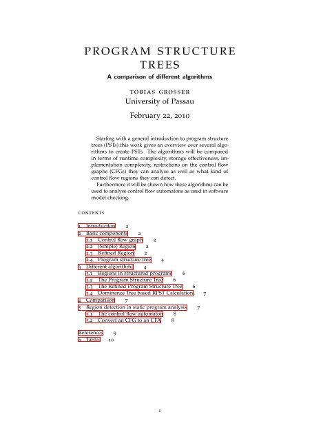
P R O G R A M S T R U C T U R E<br />
T R E E S<br />
A comparison of different algorithms<br />
tobias grosser<br />
University of Passau<br />
February 22, 2010<br />
Starting with a general introduction to program structure<br />
trees (PSTs) this work gives an overview over several algorithms<br />
to create PSTs. The algorithms will be compared<br />
in terms of runtime complexity, storage effectiveness, implementation<br />
complexity, restrictions on the control flow<br />
graphs (CFGs) they can analyse as well as what kind of<br />
control flow regions they can detect.<br />
Furthermore it will be shown how these algorithms can be<br />
used to analyse control flow automatons as used in software<br />
model checking.<br />
contents<br />
1 Introduction 2<br />
2 Basic components 2<br />
2.1 Control flow graph 2<br />
2.2 (Simple) Region 2<br />
2.3 Refined Region 2<br />
2.4 Program structure tree 4<br />
3 Different algorithms 4<br />
3.1 Regions in structured programs 6<br />
3.2 The Program Structure Tree 6<br />
3.3 The Refined Program Structure Tree 6<br />
3.4 Dominance Tree based RPST Calculation 7<br />
4 Comparison 7<br />
5 Region detection in static program analysis 7<br />
5.1 The control flow automaton 8<br />
5.2 Convert an CFG to an CFA 8<br />
References 9<br />
a Tables 10<br />
1
1 introduction<br />
Nowadays modern static analysis tools as well as optimizing compilers<br />
apply powerful optimization techniques and analysis on programs.<br />
To achieve the best results possible analysis and transformations are<br />
developed that are powerful, but often only applicable if the program<br />
to analyse fulfilles certain properties. In general a complete program<br />
does not fulfill the restrictions imposed by the intended analysis.<br />
However it is possible to extract and analyse just the regions of a<br />
program, that satisfy the required restrictions. A way to find these<br />
regions is to find all possible regions and to remove the ones, that do<br />
not satisfy the restrictions.<br />
Therefore it is interesting to understand the different algorithms<br />
available to detect the regions in a program and to investigate the<br />
(dis)advantages each of them has.<br />
2 basic components<br />
2.1 Control flow graph<br />
In compilers the code of a function as seen in Figure 1 can be described<br />
using a control flow graph (CFG) G. G = (V, E) consists of a set of<br />
vertices V, called basic blocks, and a set of edges E connecting these<br />
basic blocks. Every basic block contains a list of statements.<br />
The execution of a function is defined as a walk over the CFG, where<br />
every time a basic block is passed its statements are executed in linear<br />
order. The walk starts always at a specific basic block, the entry basic<br />
block, and ends if it arrives at a basic block, that is terminated with a<br />
”return” statement.<br />
To represent non linear control flow, branch statements may terminate<br />
a basic block. These branch statements pass, based on the result of a<br />
condition, the control to another basic block. The control flow is always<br />
following the edges of the CFG.<br />
2.2 (Simple) Region<br />
A connected subgraph of the CFG, that has only two connections to<br />
the remaining CFG, an incoming and an outcoming edge, is called a<br />
(single entry single exit) region. Such a region can be analyzed and<br />
transformed like a separate function. This can be modeled as seen in 2<br />
by replacing the orange region with a call to a function, that contains<br />
the orange CFG region. Moving or replacing the entire region is as<br />
simple as moving two edges in the CFG or if extracted as a function,<br />
changing a function call.<br />
A region is called trivial region, if it contains exactly one basic block.<br />
A region A is called canonical region, if it there is no set of regions<br />
that can be combined to construct A.<br />
2.3 Refined Region<br />
The definition of a region can be extended to a so called refined region.<br />
A refined region is a connected subgraph of a CFG, that can be transformed<br />
to a region by inserting two empty bbs, that join multiple entry<br />
or exit edges.<br />
2
int i, a, b<br />
i = 0<br />
if (i != 100)<br />
T<br />
F<br />
void foo ( ) {<br />
i n t i , a , b ;<br />
for ( i =0; i ! = 1 0 0 ; i ++) {<br />
a =3;<br />
i f ( i ==a )<br />
b =5;<br />
e lse<br />
b =8;<br />
}<br />
return ;<br />
}<br />
(a) Source code<br />
a = 4<br />
if (i == a)<br />
T<br />
F<br />
b = 5 b = 8<br />
i++<br />
(b) Control flow graph<br />
return<br />
Figure 1: A simple function<br />
int i, a, b<br />
i = 0<br />
entry<br />
if (i != 100)<br />
T<br />
F<br />
a =4<br />
if (i == a)<br />
T<br />
F<br />
a =4<br />
if (i == a)<br />
T<br />
F<br />
return<br />
int i, a, b<br />
i = 0<br />
b = 5 b = 8<br />
b = 5 b = 8<br />
exit<br />
if (i != 100)<br />
T<br />
F<br />
i++<br />
i++<br />
region(i, a, b)<br />
return<br />
return (i, a, b)<br />
(a) Region in foo()<br />
(b) Region replaced<br />
(c) Function ”orange()”<br />
Figure 2: Extracting a region into a function<br />
3
a<br />
b<br />
t_1<br />
entry<br />
a<br />
entry<br />
b<br />
entry<br />
c<br />
T F<br />
T<br />
c<br />
F<br />
d<br />
e<br />
d<br />
e<br />
t_2<br />
exit<br />
exit<br />
exit<br />
g<br />
g<br />
(a) Refined region<br />
(b) After transformation<br />
Figure 3: Transform an extended region to a plain region<br />
Every region is also a refined region. The definitions for trivial and<br />
canonical regions also apply to refined regions.<br />
An analysis of the Polyhedron 1 benchmark showed that only about<br />
30% of all refined regions are simple regions. The complete analysis<br />
can be found in Table 2.<br />
2.4 Program structure tree<br />
In general there are multiple canonical regions in every CFG. Two<br />
canonical regions A and B may contain the same basic blocks. In this<br />
case either region A is completely contained in region B, such as all<br />
basic blocks in A are also in B, or B is completely contained in A.<br />
This relationship is represented as a program structure tree, where a<br />
region B is an ancestor of A, if B is completely contained in A.<br />
The example in 4 shows a CFG where the simple regions are marked<br />
with blue and the refined regions with orange borders.<br />
3 different algorithms<br />
There are different algorithms available, that can be used to analyze a<br />
CFG and build a region tree. They differ in the CFGs they can analyze,<br />
the kind of region they can detect, as well as the implementation afford<br />
necessary, the runtime complexity and/or the required prerequisites.<br />
1 http://www.polyhedron.com<br />
4
a<br />
g<br />
h<br />
b<br />
l<br />
j<br />
i<br />
f<br />
k<br />
c<br />
d<br />
e<br />
Figure 4: Program structure tree with simple regions (blue) and refined<br />
regions (orange).<br />
5
3.1 Regions in structured programs<br />
Obtaining an region tree of a structured annotated program is trivial.<br />
Every loop and every condition is a region. The nesting of the region<br />
tree is equivalent to the nesting of the loops and conditions in the<br />
original program.<br />
Therefore this approach is taken in several algorithms, without explicitally<br />
specifying it as an region detection algorithm.<br />
However as soon as more complicated constructs like loops with<br />
multiple exits (breaks), exceptions or even gotos appear this approach<br />
does not work any more. Unfortunately many programming languages<br />
allow at least some of these constructs so a more general approach is<br />
necessary.<br />
3.2 The Program Structure Tree<br />
The in [4] published algorithm nowadays can be seen as the classical<br />
approach to calculated region trees, or as they are called in this paper,<br />
program structure trees (PST) for a general, possibly irreducible, CFG.<br />
One reason for this is the fast and streigtforward algorithm.<br />
Based on a simple data structure, called bracket list, the CFG is<br />
analysed without any previous information required. The runtime is in<br />
O(V + E).<br />
The algorithm can detect simple regions, however no refined regions.<br />
To detect refined regions, a possible approach is to insert merge<br />
basic blocks beforehand. However is has two drawbacks. First of<br />
all, deciding where to insert merge blocks is not trivial, but probably<br />
requires some analysis. Furthermore modifiying the program often<br />
invalidates existing analysis like dominance information, and is nothing<br />
that someone wants in a production compiler.<br />
3.3 The Refined Program Structure Tree<br />
In [5] the PST approach was extended and a such called Refined Program<br />
Structure Tree (RPST) was introduced. This RPST was used<br />
to model workflows in buisness processes, however it could also be<br />
applied to control flow graphs.<br />
One of the main advantages of the RPST is the refined definition of<br />
a region, that allows not only to present simple regions with just one<br />
entry and exit edge, but also regions that still have several entry and<br />
exit edges, which could be joined to a single entry or exit edge. This<br />
refinement permits the detection of regions, that cannot be handled in<br />
a plain PST.<br />
To calculate the RPST a preliminary analysis is required to build<br />
the triconnected components of the CFG as described in [3] and corrected/improved<br />
in [2]. If this analysis is not yet available the afford<br />
required to implement the RPST construction algorithm seemd to be<br />
high, especially as the triconnected components algorithm is not trivial.<br />
Another drawback of this algorithm and the refined region definition<br />
is, that a region cannot be described in constant memory, but has to be<br />
defined by all incoming and outgoing edges. To know if a basic block<br />
is part of a region a auxilary data structure has to store a mapping in<br />
between basic blocks and regions, otherwise a graph walk is required.<br />
6
Analysis PST RPST DRPST<br />
Applicable All CFGs All CFGs All CGSs<br />
Precision Basic regions Enhanced regions Enhanced regions<br />
Runtime O(V + S) O(V + S) O((V + S) 2 ), probably<br />
better<br />
Prerequisites None Triconnected components<br />
Dominance and Postdominance<br />
trees<br />
Representation 2 edges all edges in region 2 basic blocks<br />
BB in Region extra mapping required based on dominance info<br />
Table 1: Comparison of different region detection algorithms<br />
3.4 Dominance Tree based RPST Calculation<br />
In winter 2009 another approach was developed as a region detection<br />
algorithm for the LLVM compiler toolkit. The objective was to achieve<br />
the same precision as in the previous described algorithm, but to take<br />
advantage of already existing analysis.<br />
One of the most common analysis in restructering compilers is<br />
the (post)dominance information. Therefore a relatively simple algorithm<br />
was developed, that calculates a region tree based on the<br />
(post)dominance information already available.<br />
The algorithm is able to detect all refined regions on any (even<br />
unstructured) CFG. A first analysis of the runtime complexity has<br />
shown an upper bound of O((V + S) 2 ), however it seems possible to<br />
proof even better performance in the order of magnitude of O((V +<br />
S) + log(V + S)).<br />
Another advantage of a dominance tree based approach are the<br />
constant time operations to check if a basic block is part of a region.<br />
These operations are possible, as the algorithm can take advantage<br />
of the existing (post) dominance information. This also leads to the<br />
advantage of being able to store the description of a region in a constant<br />
amount of memory, two references to a basic block.<br />
4 comparison<br />
In “Table 1” the attributes of all algorithms, that can handle general<br />
CFGs, are summed up. Because of the better precision the RPST and<br />
DRPST algorithms seem to be the most powerful analysis. In theory<br />
the RPST algorithm is already perfect in terms of runtim complexity,<br />
coverage and precision, however in practise it requires a lot of<br />
implementation afford.<br />
This problem seems to be solved by the DRPST algorithm, that can<br />
be implemented easily, if dominance information is already available.<br />
The only drawback is the not yet proven optimal runtime complexity.<br />
However in first tests a limitation because of this, was not found.<br />
5 region detection in static program analysis<br />
In static program analysis, especially software model checking, often<br />
extremly expensive analysis are performed. To get resonable runtime it<br />
is therefore necessary to reduce the affords required as much as possible.<br />
Program region trees offer various possiblities to reduce complexity.<br />
7
One possibility is to analyze different parts of a program with different<br />
accuracy, such that only interesting regions are analyzed precisely.<br />
Other regions could be analyzed roughly and, if required, be refined<br />
later.<br />
Another possiblity is to hide the complexity of a program, by considering<br />
only the overall effect of a region on the program state, but<br />
not simulating every single change that the execution of a program<br />
region implies. As the complexity of a lot of algorithms is related to the<br />
number of analyzed program states, reducing the number of program<br />
states might improve runtime significantly.<br />
5.1 The control flow automaton<br />
Static program analisis often uses a control flow automaton (CFA) to<br />
represent a program, in contrast to the CFGs that are more widespread<br />
in optimizing compilers.<br />
A control flow automaton is a graph G=(V, E) with a set of vertives V<br />
and a set of edges E. Every vertice represents a program state. Transitions<br />
in between program states are defined by the edges, that connect<br />
two states applying an operation. The operations can be either a set of<br />
calculations or a assume operation.<br />
5.2 Convert an CFG to an CFA<br />
To convert an CFG to an CFA as seen in 5 it is necessary to find the<br />
program states and transitions in an CFG. In a CFG the program state<br />
is changed by the operations executed in the basic blocks. Before and<br />
after the operations in a basic block, there is a defined program state.<br />
Therefore we can create for every basic block BB two new program<br />
states c 1, c 2 one defining the state before and one after the execution of<br />
BB. The transition between these two program states can be defined as<br />
execution of the operations contained in the basic block. If a terminating<br />
branch statement exists in the basic block, the conditions can be applied<br />
as assume operations on the transitions from c 2 to the next program<br />
states.<br />
8
a<br />
b<br />
a<br />
b<br />
c_1<br />
i = 100<br />
i=100<br />
if (b == 80)<br />
T<br />
F<br />
c_2<br />
b == 80<br />
b != 80<br />
d<br />
e<br />
d<br />
e<br />
(a) CFG<br />
(b) CFA<br />
Figure 5: Convert a CFG basic bock to CFA nodes and transitions<br />
references<br />
[1] Thomas Ball. What’s in a region?: or computing control dependence<br />
regions in near-linear time for reducible control flow. ACM Lett.<br />
Program. Lang. Syst., 2(1-4):1–16, 1993.<br />
[2] Carsten Gutwenger and Petra Mutzel. A linear time implementation<br />
of spqr-trees. In GD ’00: Proceedings of the 8th International Symposium<br />
on Graph Drawing, pages 77–90, London, UK, 2001. Springer-Verlag.<br />
[3] John E. Hopcroft and Robert Endre Tarjan. Dividing a graph into<br />
triconnected components. SIAM J. Comput., 2(3):135–158, 1973.<br />
[4] Richard Johnson, David Pearson, and Keshav Pingali. The program<br />
structure tree: Computing control regions in linear time. pages<br />
171–185, 1994.<br />
[5] Jussi Vanhatalo, Hagen Völzer, and Jana Koehler. The refined<br />
process structure tree. In BPM ’08: Proceedings of the 6th International<br />
Conference on Business Process Management, pages 100–115, Berlin,<br />
Heidelberg, 2008. Springer-Verlag.<br />
9
a<br />
tables<br />
Program Plain Extendable Plain / Extandable<br />
ac.s 65 77 0.84<br />
aermod.s 1069 5262 0.20<br />
air.s 255 486 0.52<br />
capacita.s 102 232 0.44<br />
channel.s 56 69 0.81<br />
doduc.s 241 702 0.34<br />
fatigue.s 44 133 0.33<br />
gas dyn.s 76 219 0.35<br />
induct.s 66 239 0.28<br />
linpk.s 44 99 0.44<br />
mdbx.s 84 272 0.31<br />
nf.s 57 122 0.47<br />
protein.s 93 313 0.30<br />
rnflow.s 291 786 0.37<br />
test fpu.s 242 650 0.37<br />
tfft.s 24 58 0.41<br />
Sum 2809 9719 0.29<br />
Table 2: Regions in the polyhedron.com benchmark<br />
10