FHA Signal Timing On A Shoestring

SIGNAL TIMING 

ON A SHOESTRING 

Publication Number: FHWA-HOP-05-034 

TASK ORDER UNDER CONTRACT NUMBER: DTFH61-01-C-00183 

MARCH 2005

Notice 

This document is disseminated 

under the sponsorship of the 

Department of Transportation in 

the interest of information 

exchange. The United States 

Government assumes no liability 

for its contents or use thereof.

Technical Report Documentation Page 

1. Report No. 

FHWA-HOP-05-034 

4. Title and Subtitle 

Signal Timing on a Shoestring 

2. Government Accession No. 3. Recipient's Catalog No. 

5. Report Date 

March, 2005 

6. Performing Organization Code 

7. Author(s) 

Henry, RD 

9. Performing Organization Name and Address 

Sabra,Wang & Associates, Inc. 

1504 Joh Avenue, Suite 160 

Baltimore, MD 21227 

8. Performing Organization Report No. 

10. Work Unit No. (TRAIS) 

11. Contract or Grant No. 

12. Sponsoring Agency Name and Address 

Office of Travel Management 

Federal Highway Administration 

400 Seventh Street 

Washington, DC 20590 

13. Type of Report and Period Covered 

14. Sponsoring Agency Code 

15. Supplementary Notes 

COTR: Pamela Crenshaw, John Halkias 

Reviewers: Mike Shauer, Ed Fok 

16. Abstract 

The conventional approach to signal timing optimization and field deployment requires current 

traffic flow data, experience with optimization models, familiarity with the signal controller 

hardware, and knowledge of field operations including signal timing fine-tuning. Developing new 

signal timing parameters for efficient traffic flow is a time-consuming and expensive undertaking. 

This report examines various cost-effective techniques that can be used to generate good signal 

timing plans that can be employed when there are insufficient financial resources to generate the 

plans using conventional techniques. The report identifies a general, eight-step process that leads 

to new signal plans: 1) Identify System Intersections; 2) Collect and Organize Existing Data; 3) 

Conduct a Site Survey; 4) Obtain Turning Movement Data; 5) Calculate Local Timing Parameters; 

6) Identify Signal Groupings; 7) Calculate Coordination Parameters; and, 8) Install and Evaluate 

New Plans. The report examines each of these steps and identifies procedures that can be used to 

minimize costs in each step. Special emphasis is placed on the costs of turning movement counts. 

The report develops a “tool box” of procedures and provides examples of how the tool box can be 

used when there is a moderate signal timing budget; when there is a modest signal timing budget; 

and when there is a minimum signal timing budget. 

17. Key Word 

Signal timing, turning movement data, signal 

timing optimization, time-space diagrams, 

manual methods, cycle, split, offset. 

18. Distribution Statement 

19. Security Classif. (of this report) 20. Security Classif. (of this page) 21. No. of 

Pages 

22. Price 

Form DOT F 1700.7 (8-72) 

Reproduction of completed page authorized 

i

Table of Contents 

I. Introduction...........................................................................................................................1 

Intended Audience...............................................................................................................1 

Classical Signal Timing Process .........................................................................................2 

Data Collection ..............................................................................................................2 

Optimization..................................................................................................................5 

Installation and Evaluation (Field Adjustments).........................................................7 

Report Structure..................................................................................................................7 

II. Signal Timing Process .........................................................................................................9 

1 - Identify the System Intersections ..................................................................................9 

2 - Collect and Organize Existing Data ..............................................................................9 

3 - Conduct Site Survey.....................................................................................................10 

4 - Obtain Turning Movement Data..................................................................................12 

5 - Calculate Local Timing Parameters ............................................................................12 

6 - Identify Signal Groupings ............................................................................................12 

7 – Calculate Coordination Parameters............................................................................13 

8 - Install and Evaluate New Plans ..................................................................................13 

III. Signal Timing Tool Box ....................................................................................................15 

Data Collection Tools.........................................................................................................15 

Intersection Categorization.........................................................................................15 

Short Count Method ....................................................................................................16 

Estimated Turning Movements ..................................................................................17 

Signal Grouping.................................................................................................................17 

Coupling Index ............................................................................................................17 

Major Traffic Flows .....................................................................................................19 

Coordinatability Factor ...............................................................................................19 

Number of Timing Plans ...................................................................................................19 

Cycle Length Issues...........................................................................................................20 

Webster’s Equation......................................................................................................20 

Greenshields-Poisson Method .....................................................................................21 

Cycle Length................................................................................................................22 

iii

Offset Issues ......................................................................................................................24 

One-way Offset ............................................................................................................25 

Two-Way Offsets (Kell Method) ..................................................................................26 

Split Issues ........................................................................................................................28 

Critical Movement Method..........................................................................................28 

IV. Local Controller Parameters ............................................................................................30 

Actuated Controller Timing Principles .............................................................................30 

Basic Actuated Phase Settings..........................................................................................31 

Minimum Green (Initial).............................................................................................31 

Extension (Passage).....................................................................................................32 

Maximum Green..........................................................................................................32 

Yellow ..........................................................................................................................33 

Red ...............................................................................................................................33 

Pedestrian Parameters......................................................................................................33 

Walk.............................................................................................................................34 

Flashing Don’t Walk....................................................................................................34 

Volume-Density Phase Settings........................................................................................34 

Variable Initial ............................................................................................................34 

Gap Reduction .............................................................................................................35 

Controller Timing Parameters Summary .........................................................................35 

V. Coordination Timing Issues...............................................................................................37 

Resonant Cycle ..................................................................................................................37 

Intersection Categories .....................................................................................................38 

Number of Timing Plans ...................................................................................................39 

Using the Tool Box ............................................................................................................39 

VI. Signal Timing Examples ..................................................................................................41 

Moderate Signal Timing Budget .......................................................................................41 

1 - Identify the System Intersections ..........................................................................41 

2 - Collect and Organize Existing Data ......................................................................41 

3 - Conduct Site Survey...............................................................................................41 

4 - Obtain Turning Movement Data............................................................................42 

5 - Calculate Local Timing Parameters ......................................................................42 

6 - Identify Signal Groupings ......................................................................................42 

7 - Calculate Coordination Parameters.......................................................................42 

iv

8 - Install and Evaluate New Plans ............................................................................42 

Modest Signal Timing Budget...........................................................................................43 









Minimum Signal Timing Budget ......................................................................................45 









v

I. Introduction 

Research and experience has shown that retiming traffic signals is one of the most costeffective 

tasks that an agency can do to improve traffic flow. Traffic flow improvements of 

up to 26% have been reported 1 . In spite of this potential, many Traffic Engineers simply do 

not have the budgetary resources to conduct a signal retiming program using the 

conventional methods. 

The conventional approach to signal timing optimization and field deployment requires 

current traffic flow data, experience with optimization models, familiarity with the signal 

controller hardware, and knowledge of field operations including signal timing fine-tuning. 

To many practitioners, this is a daunting process best left as something to be done by others 

at a time in the indefinite future. Setting new signal timing parameters for efficient traffic 

flow is time-consuming and expensive. Typically, this process involves five distinct steps: 

 

 

 

 

 

Organizing existing information, 

Collecting new traffic flow data in the field, 

Coding and running signal timing optimization program(s), 

Validating and selecting optimum signal timing settings, and 

Installing and fine-tuning new signal timing plans in signal controllers in the street. 

There are, however, practitioners in the field who have developed practical and costeffective 

means to short-cut these tasks, but yet generate signal timing plans that can 

approximate the effectiveness of signal timing developed using the formal modeling process. 

We refer to these plans as “near-optimum” plans. It is not reasonable to expect the same 

quality signal timing output from a short-cut method as one would expect from the formal, 

costly process. However when faced with a lack of resources such that signal timing by 

conventional means is not possible, these short cut methods should be considered rather 

than not retiming the signals. 

This report examines the informal traffic signal timing process and defines the various 

methods that can be used to minimize the cost of generating near-optimum signal timing 

settings. This effort places a primary emphasis on updating the signal timing in an arterial 

corridor. In short, this effort investigates how signal timing plans can be developed and 

updated efficiently at the lowest possible cost. 

Intended Audience 

The intended audience for this report includes Administrators, Managers, Engineers, and 

Technicians who are trying to maintain the best possible signal settings with less than 

optimum budgets. The report assembles a body of knowledge related to signal timing that 

is structured in a way that will be useful to those who are responsible for making the 

constant signal timing adjustment that are required to meet the ever increasing traffic 

demands. 

1 

“Managing Traffic Flow through Signal Timing;” S. Lawrence Paulson; Public Roads; January/February 2002; Vol. 65No. 4. 

1

Classical Signal Timing Process 

Signal timing is a task that frequently involves coordinating activities from many different 

departments of the jurisdiction. It is not unusual for the traffic counts and mapping data to 

be provided by the Planning Department, the timing optimization analysis to be conducted 

by the Traffic Engineering Department, with the actual parameter installation being done 

by the Maintenance Shop. It is important to recognize that the signal timing process is not 

simply executing a computer program; rather, it is a continuing series of tasks that involve 

persons with many different skills. Two of the most prominent are the traffic engineer and 

the traffic signal technician. The engineer typically uses a software model, like Passer-II or 

Synchro to derive the timing plan which is defined in terms of a cycle length, split, and 

offset. These data are then provided to the traffic signal technician who must convert these 

variables into the timing parameters used by the controller. 

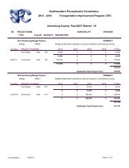
It is useful to examine the entire signal timing process as it is commonly practiced today in 

many cities and counties. The complete process is probably more complex than one might 

expect. Figure 1 illustrates the major activities and interfaces that are typically followed to 

update signal settings. Whether the process is applied to a single intersection or to an 

entire city, the steps are the same. It is also interesting to note that that the same steps 

must be followed whether the process is entirely manual or completely automated. Each of 

the major activities of the signal timing process is described below. 

In the real world, the signal timing process begins with a “Trigger Event”. This event may 

be as benign as a scheduled activity to retime the controller every few years. More likely, 

however, the impetus for new signal timing is a citizen complaint (“The light is too short”); 

a major change in the road network (widening of the existing arterial); or a significant 

change in demand (opening of a shopping center). Whatever the cause, the initial response 

is usually a review of the existing timing and equipment to make sure the there is no 

hardware failure. One of the most common signal timing complaints is that the phase time 

is too short. This is frequently a result of a detector malfunction. This initial response, 

then, is to affirm that the hardware is operational and the timing parameters are operating 

as planned. After the Trigger Event, there are two basic paths through the process: Field 

Adjustments and System Retiming. 

The “Field Adjustment” path is shown in Figure 1 as the path directly down from the 

“Determine Type of Timing Problem” box. This path is entirely empirical and intuitive and 

produces results only as good as the experience of the person doing the adjustments. The 

other path is the one on which we will focus most of our attention. This path begins with a 

data collection effort and continues through an optimization process to generate and install 

new system timing parameters. There are three primary activities involved in the Classical 

Signal Timing Process: Data Collection, Optimization, and Installation/Evaluation. 

Data Collection 

Of course, signal retiming is not about making simple adjustments to a few timing 

parameters in a controller. Most jurisdictions follow a more complicated effort to retime a 

signal or group of signals using modern computer programs and procedures. This path is 

the somewhat more complex activities that are indicated on Figure 1 to the right of the 

“Field Adjustment” path. There are two broad categories of data that are required by the 

process; turning movement counts and network descriptive data. It is stressed that the 

user must maintain accurate records of all timing input data for this process to be effective. 

2

Trigger Event 

Determine 

Type of Timing 

Problem 

Field 

Adjustment 

? 

No 

Current 

Count Data 

? 

Yes 

Current 

Descriptive 

Data ? 

Yes 

No 

No 

Adjust 

and 

observe 

Turning 

Movement 

Counts 

Field 

Inventroy 

Yes 

No 

Looks 

OK 

? 

Prepare 

Optimization 

Program 

Input 

Yes 

Parameter Changes 

Time and Date 

Manually Recorded 

Enter Data 

Into 

Controller 

Run 

Optimization 

Program 

Identify 

Problem 

Convert 

Output to 

Controller 

Format 

Results 

Look 

OK 

? 

No 

Yes 

Timing Process 

Complete 

Figure 1. Classical Approach to Signal Timing. 

3

Turning Movement Counts 

This path through the flow chart begins with a determination of whether 

there is adequate traffic count data. For the most part, the need is for 

turning movement counts that reflect the traffic demand. Most Traffic 

Engineers consider four plans to be the minimum required for proper signal 

operation: AM Peak Plan, Day Plan, PM Peak Plan, and the Night Plan. A 

basic need, therefore, is to have a turning movement count for each of these 

four periods. In areas near major shopping venues there may be additional 

needs for unique timing plans that are related to shopping demand. 

While this seems simple enough, it is not inexpensive. Collecting these data 

typically costs in the range of $500 to $1,000 per intersection or more. 

Converting the raw count data into a format useful for analysis easily can 

double the cost. This is an area where significant progress has been made. 

For example one vendor, Jamar Technologies Inc., makes an electronic data 

collection board that is easy to use, accurate, and reliable. Although an 

observer is still required to record the movements, once the observations are 

completed, the data are easily uploaded to a computer for further processing. 

The more elegant solution to this problem, however, is to collect the data 

using existing system and local detectors and to derive a complete traffic 

volume network with all turning movement from these detector data. 

Several systems, QuicNet/4, MIST, Pyramids, and Actra (probably there are 

others) have the capability to export traffic count data from existing count 

stations. The missing capability is to be able to use this information to build 

a complete network turning movement schedule. 

Traffic count data must be considered in two dimensions, temporal and 

spatial. In the temporal dimension, traffic count data at any one point varies 

from period to period as traffic demand ebbs and flows. In the spatial 

dimension, we frequently require traffic count data at many different 

intersections for the same time period. In addition, to accommodate certain 

flows through a series of intersections, we need to know the upstream origin 

of the demand for each turning movement at the downstream intersection. 

The need for traffic counts is not a unique demand for signal timing; most 

Traffic Engineering endeavors require traffic count information. Traffic 

signal timing, however, does require accurate turning movement counts. 

Turning movement counts (or estimates) are fundamental to developing 

timing plans. These counts must be estimated in such a way as to represent 

traffic demand. In other words, one must be sure that the count information 

truly represents traffic demand and not just the traffic that was able to get 

through the intersection with the existing signal settings. A related issue to 

be aware of is the possibility that the traffic counted on a particular approach 

is actually constrained by the signal settings at the upstream intersection 

feeding that approach. 

4

Descriptive Data 

All signal optimization and simulation models, even manual signal timing 

procedures, require a physical description of the network. This description 

includes distance between intersections (link length), the number of lanes, 

lane width and grade, permitted traffic movements from each lane, and the 

traffic signal phase that services the flow. Building a network from scratch is 

a significant undertaking. But once the network is defined; in general, only 

traffic demand and signal timing parameters have to be updated to test a 

new scenario. 

An implied issue that is addressed in this step is to identify which 

intersections are to be included in the system. While this is a trivial issue for 

many simple networks, it can be a difficult problem to resolve in the more 

complex networks. In general, signals should operate as a system when 

adjacent intersections have similar cycle length requirements and there are 

significant benefits to be derived from controlling the offset. When the cycle 

length requirements are within 15 seconds of one another and the distance 

between intersections is less than 0.5 miles, many Traffic Engineers feel that 

the signals should be coordinated. These issues will be explained in more 

detail in later sections of this document. 

Optimization 

Once the data are collected, the final step is to generate the optimized signal 

settings. While this task can be accomplished manually, and in later sections of this 

report, we will describe some manual techniques that can be used, most Engineers 

use a computer program. There are a number of computer programs that can be 

used to generate signal timing parameters. These programs can be placed into one 

of two categories: those developed by the private sector and those developed by the 

public sector. The programs developed by the private sector tend to be more 

expensive to purchase but also tend to be updated more frequently. The programs 

developed by the public sector tend to be more thoroughly vetted by the research 

community. Three of the more popular programs of this type are Synchro, Passer II, 

and Transyt-7F. The Federal Highway Administration Traffic Analysis Toolbox 

(http://ops.fhwa.dot.gov/Travel/Traffic_Analysis_Tools/tat_vol2/sectapp_e.htm#secta 

ppe_4) provides additional resources. 

Synchro 

Synchro is a macroscopic traffic signal timing tool that can be used to 

optimize signal timing parameters for isolated intersections, for arteries, and 

for networks. It produces useful time-space diagrams for interactive finetuning. 

Synchro can analyze fully actuated coordinated signal systems by 

mimicking the operation of a NEMA controller, including permissive periods 

and force-off points. Using a mouse, the user can draw either individual 

intersections or a network of intersecting arteries, and also can import .DXF 

map files of individual intersections or city maps. The program has no 

limitations on the number of links and nodes. 

Synchro is designed to optimize cycle lengths, splits, offsets, and left-turn 

phase sequence using proprietary logic. The program also optimizes multiple 

5

cycle lengths and performs coordination analysis. When performing 

coordination analysis, Synchro determines which intersections should be 

coordinated and those that should run free. The decision process is based on 

an analysis of each pair of adjacent intersections to determine the 

“coordinability factor” for the links between them. 

Synchro calculates intersection and approach delays either based on the 

Highway Capacity Manual (HCM) or a proprietary method. The major 

difference between the HCM method and the Synchro method is treatment of 

actuated controllers. The HCM procedures for calculating delays and LOS 

are embedded in Synchro; thus, the user does not need to use HCM software. 

Synchro has unique visual displays, including an interactive traffic flow 

diagram. The user can change the offsets and splits with a mouse, then 

observe the impacts on delay, stops, and LOS for the individual intersections, 

as well as the entire network. 

Passer II 

Passer II (Progression Analysis and Signal System Evaluation Routine) was 

originally developed in 1974 by the Texas Transportation Institute (TTI). 

Passer II is an arterial-based, bandwidth optimizer, which determines phase 

sequences, cycle length, and offsets for a maximum of 20 intersections in a 

single run. Splits are determined using an analytical (Webster’s) method, but 

are fine-tuned to improve progression. Passer II assumes equivalent pretimed 

control. 

Passer II requires traffic flow and geometric data, such as design hour 

turning volumes, saturation flow rates, minimum phase lengths, distances 

between intersections, cruise speeds, and allowable phase sequencing at each 

intersection. The Passer II timing outputs include: design phase sequences, 

cycle length, splits, and offsets, and includes a time-space diagram. 

Performance measures include volume-to-capacity ratio, average delay, total 

delay, fuel consumption, number of stops, queue length, bandwidth efficiency, 

and level of service. In addition to the time-space diagram, Passer II has a 

dynamic progression simulator, which lets the user visualize the movement of 

vehicles along the artery using the design timing plan. 

There are two other versions of Passer that are available, Passer III and 

Passer IV. Passer III is a diamond interchange signal optimization program 

and Passer IV is a program that is used to optimize a network of traffic signals 

which is based on maximing bandwidths. 

Transyt-7F 

Transyt-7F (TRAffic Network StudY Tool, version 7, Federal) is designed to 

optimize traffic signal systems for arteries and networks. The program 

accepts user inputs on signal timing and phase sequences, geometric 

conditions, operational parameters, and traffic volumes. Transyt-7F is 

applied at the arterial or network level, where a consistent set of traffic 

conditions is apparent and the traffic signal system hardware can be 

integrated and coordinated with respect to a fixed cycle length and 

6

coordinated offsets. Although Transyt-7F can emulate actuated controllers, 

its application is limited in this area. 

Transyt-7F optimizes signal timing by performing a macroscopic simulation 

of traffic flow within small time increments while signal timing parameters 

are varied. Design includes cycle length, offsets, and splits based on 

optimizing such objective functions as increasing progression opportunities; 

reducing delay, stops, and fuel consumption; reducing total operating cost; or 

a combination of these. 

Unique features of Transyt-7F include the program’s ability to analyze 

double cycling, multiple greens, overlaps, right-turn-on-red, non-signalized 

intersections, bus and carpool lanes, “bottlenecks,” shared lanes, mid-block 

entry flows, protected and/or permitted left turns, user-specified bandwidth 

constraints, and desired degree of saturation for movements with actuated 

control. Other applications of the tool include evaluation and simulation of 

“grouped intersections” (such as diamond intersections and closely-spaced 

intersections operating from one controller) and sign-controlled intersections. 

Of course, this power and flexibility comes with a price. This is by far the 

most complex program to set up and use. It is also the most expensive to use 

and probably not the best selection for developing signal timing plans with a 

minimum budget. 

Installation and Evaluation (Field Adjustments) 

Once the hardware is determined to be operating correctly, the last task is to 

evaluate how well the new signal settings are managing traffic demand. Notice that 

the two paths through the flow chart shown in Figure 1. Many times, a simple 

adjustment of one parameter may be all that is necessary. It may be possible to 

accommodate longer queues on the main street, for example, by simply advancing 

the Offset by several seconds. Other timing problems can be resolved by simple 

adjustments to the Minimum Green or Vehicle Extension parameters. These types 

of issues are resolved by a positive output from the “Field Adjustment” decision in 

Figure 1. In most jurisdictions, the entire sequence, from determining the type of 

problem, to making the adjustments, to evaluating the results, to recording the 

changes is a manual process that relies on the experience of a Signal Engineer (or 

Signal Technician) to provide a solution. Obviously, the quality of the solution is a 

function of the experience and dedication of the person doing the work. 

Report Structure 

In addition to this introductory section, the report has five sections. Section 2 defines the 

eight steps that are common to any signal retiming effort, whether it is for one signal or for 

a system of hundreds of signals. Of importance in reviewing these steps is to recognize that 

they exist whether they require any resources with the current effoto rt or not. 

This report provides a number of “rules of thumb” and methods that may be used to 

estimate various values that are used in the signal timing process. We caution the user to 

follow suggestions when appropriate, but to be aware that it is always desirable to verify 

these estimates with field observations when possible. 

7

The following section provides a “tool box” of resources for the Practitioner. These 

resources will aid the user in collecting and managing data, in better understanding the 

physical constraints involved with signal timing, and explain back-of-the-envelope 

techniques that may be used when cost constraints prohibit more traditional solutions. 

Signal settings can be categorized as local controller parameters or coordination 

parameters. The local controller parameters include phase minimums, extension times, 

and change and clearance intervals. Coordination parameters are the Cycle Length, Split 

and Offset. The Local Controller parameters are presented in Section 4 and the 

Coordination issues are discussed in Section 5. The report concludes with three examples 

of how these techniques can be applied. One scenario involves an agency that has funds for 

signal timing but does not have enough resources to complete the classical method. The 

second scenario illustrates how an agency can develop signal settings with a modest budget, 

and the third scenario illustrates what an agency can do with virtually no budget for signal 

timing other than the part time effort from existing staff. 

8

II. Signal Timing Process 

There are eight distinct steps that define the signal timing development process. Not every 

step requires a costly effort to complete in every instance. For example, it is not difficult to 

determine the signal grouping for an arterial with three signals. It may be a somewhat 

more difficult task to identify signal groupings for 50 intersections in arterial and grid 

networks. The steps begin with identifying the system boundaries. This boundary helps to 

minimize the scope-creep temptation of adding just one more intersection. From here the 

steps are a logical and straightforward process that will enable the Practitioners to 

efficiently acquire only the essential information. This methodical procedure will enable 

Practitioners to avoid one of the most costly endeavors – making a second or third trip to 

the field to obtain more data, or data that was missed this first time. 

1 - Identify the System Intersections 

Although this step is obvious, it is a necessary first step. The intent is to clearly identify all 

intersections that will be analyzed in the effort. This is an important issue because all 

intersections will require a base-line amount of attention at the start of the effort. This 

effort translates to a cost which we want to minimize. 

Each intersection must be identified by a unique name and number. It will be helpful if the 

numbering scheme is organized in a way that reflects the geometry of the intersections. 

For example, if the intersections are on an arterial that generally runs east and west, the 

numbers might start with the lowest number for the western most intersection and 

increase to the east. Other basic information should be defined at this time including 

whether the intersection is currently signalized, political jurisdiction, responsible 

maintenance organization and any other general, readily-available information or 

characteristic. This information should be entered into a spreadsheet. 

It is important to recognize at this point that this listing is all intersections that are under 

consideration. This does not imply that all of these intersections will necessarily operate 

together as a group or system; it simply means that these intersections will be considered 

and evaluated. Some or all may operate together as a single group, or we may operate 

them as two or more separate groups, or we may find that one or more intersections will 

operate better as isolated intersections. These solutions can only be evaluated after an 

operational analysis. 

2 - Collect and Organize Existing Data 

The data needed to prepare signal timing plans can be divided into two categories, 

descriptive and demand. The descriptive data is the easiest to obtain; and, for the most 

part, can be obtained from the files of the operating agency. These data include the 

following: 

 

A condition diagram of each intersection showing the number of lanes and width of 

each lane on all approaches. The condition diagram must have a North arrow and 

show the street names. 

9

A phasing diagram for intersections with existing controllers. It is important for the 

phasing diagram to include the NEMA phase number for each phase movement. 

The phasing diagram must also show all overlaps (if any). 

Existing detector location, type (presence or passage), and phase assignment 

information. These data are necessary to determine the phase interval settings like 

the minimum green and the extension. 

Existing traffic count data. The most useful data are turning movement counts. 

When using old counts, it is necessary to determine if there has been any major 

change in the traffic demand since the count was made. If there has been no 

significant change in demand, then the counts can be adjusted for annual traffic 

growth. If there has been a major change, then the counts may not be as useful. 

Hourly road tube counts and even Average Annual Daily Traffic 24-hour counts are 

also useful information and can be used to estimate traffic growth and even estimate 

turning movement counts. This information may be available from the local 

jurisdiction, from the local or regional planning agencies, and from the state DOT. 

Because manual counting is the single most expensive element to signal timing, a 

major effort to assimilate existing data is usually well worth the effort and cost. 

Distance between intersections and the free-flow travel speed for the conditions 

under which the timing plan will operate. This information should be depicted of a 

map of the area showing the roads and signalized intersections. It is not necessary 

for the map to be drawn to scale, it is important for each link on the map to be long 

enough to be able to show various data such as link length, speeds, and volume. 

An estimate of the number of different timing plans that may be needed and the 

times during which each plan would be used. This information must be determined 

based on the available traffic count data and the experience of the Practitioner 

3 - Conduct Site Survey 

This step may be the most important step in the process. Although it is possible to 

generate both local and coordinated signal timing parameters without ever seeing the 

intersection, this is a very dubious practice. Physical constraints which may or may not be 

noted on a plan sheet, but may have an obvious impact on traffic flow are immediately 

obvious to the viewer. Vegetation sight distance obstructions, adverse approach grades and 

curvature, and fading pavement markings are examples of factors that affect traffic flow 

which are apparent during a site survey. 

The site survey is most effective when conducted after all of the existing data has been 

collected and organized. The purpose of the site visit is to confirm the existing information 

gathered in the previous step is accurate and to collect any additional data that may be 

needed. 

It is strongly recommended that each intersection be visited during the hours for which the 

timing plan is being developed. For example, if four timing plans are being developed, then 

the intersection should be visited during the AM Peak, during a typical day period, during 

the PM Peak, and during a low-volume night period. Most of the information will be 

obtained during the typical day period, but site visits during the extreme conditions of both 

high and low volume will frequently provide an insight into signal operation that cannot be 

obtained any other way. 

10

The basic intersection checklist includes the following: 

 

 

 

 

 

Condition Diagram – This may be a verification of the intersection sketch 

obtained during the previous step, or if there is no existing drawing, a new diagram 

must be prepared. This diagram should include the following: 

o 

o 

o 

o 

Intersection sketch showing driveway curb cuts, sidewalks, crosswalks, North 

arrow, street names. 

Approach lane configurations including widths and movement assignments. 

Sight distance restrictions and cause such as vertical or horizontal curvature, 

and vegetation. 

Curb restrictions (parking, loading zone, transit stop, etc.) 

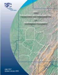
Phasing Diagram – Like the 

Condition Diagram, this diagram is 

either a verification of existing 

information or the preparation of a 

new document. It is important for the 

phasing diagram to include the 

NEMA phase number for each phase 

movement and to identify the NEMA 

phase number with the corresponding 

traffic movement by direction. For 

example, Eastbound Left Turn – 

Phase 5; Eastbound Through – Phase 

2. The phasing diagram must also 

show and identify all overlaps (if any). 

Example 4 Standard 

8-Phase Intersection, Layout 

Session 4 

5 

2 

4 7 

3 8 

6 

1 

1 

5 

NHI 133028 Traffic Control Signalization and 

Software 

2 

6 

Main Street 

Barrier 

3 4 

7 8 

Side Street 

Detector Locations - Existing detector location, type (presence or passage), and 

phase assignment data are necessary to determine the phase interval settings. The 

purpose of the field visit is to verify that the detectors are deployed as shown on 

existing documents; but more importantly, the purpose is to verify that the detectors 

are operating as designed. 

Existing Controller Settings – With modern controllers, it is not unusual to find 

three distinctly different sets of local controller timing data: the data in the 

controller itself; the data shown on intersection records in the controller cabinet; and 

controller data from the office records. Of course the purpose of the site visit is to 

reconcile any differences among these record sets and to verify that the settings are 

reasonable for the traffic conditions. 

Traffic Flow Observations – While visiting each intersection, record the typical 

free flow speed observed on each link and record this information on the map 

prepared in the previous step. Notice that the speeds may be different for each 

timing plan. This observation is important because it will have a major impact on 

the offset. It is also practical to determine the link length using the vehicle’s 

odometer to verify the information recorded on the map. This independent 

verification of link length could save a great deal of work that would be required if 

the distance recorded on the map were wrong. 

11 

11

For this minimum cost approach to signal timing to be effective, it is vitally important to 

make full use of all existing information. At this point in the process, the Practitioner will 

be able to observe the operation of the intersection during the time period of interest with 

full knowledge of the existing parameters and detector operation. While it would be 

valuable to be able to use an analytical tool to evaluate intersection performance, the lowbudget 

approach cannot support this luxury. Instead, the observations and experience of 

the Practitioner are substituted. 

4 - Obtain Turning Movement Data 

This step involves the preparation of turning movement data for each Primary intersection 

for each timing plan to be developed. The following options are available to the 

Practitioners to acquire these data listed in descending order of expected accuracy. 

1. Conduct a new turning movement count for the period in question. 

2. Conduct a “Short Count” using the procedures discussed in the following Section. 

3. At an intersection where there has been no significant construction or development, 

update an old turning movement count to reflect general traffic trends. 

4. Estimate turning movement data using the methods discussed in the following 

Section that are based on NCHRP 255, “Highway Traffic Data for Urbanized Area 

Project Planning and Design”. This effort may be performed using the program, 

TurnsW 2 which estimates turning volumes from existing link volumes. 

5 - Calculate Local Timing Parameters 

As previously noted, it is not unusual to find conflicting information concerning controller 

parameters among the various record sets in the office and in the field. It is assumed that 

the field observations have identified a situation whereby the local controller settings 

require a revision to improve the intersection performance. This step represents the work 

necessary to revise existing local controller operation parameters. 

The local operation parameters are the settings like phase minimums, maximums, change, 

and clearance intervals. These settings are primarily a function of traffic demand, the 

geometric design of the intersection, and the type and location of detectors. 

6 - Identify Signal Groupings 

At this point in the signal timing process, all of the intersections should be operating 

efficiently as isolated intersections. In other words, each intersection should be processing 

the local demand. Of course, operating efficiently as an isolated intersection and operating 

efficiently as a system are two entirely different situations. 

The purpose of this step is to identify groups of signalized intersections that should operate 

together as a coordinated unit. One constraint of grouping signals is that all controllers in 

a group must operate on the same cycle length. It is likely that the cycle length 

requirements for different intersections are not always identical. A trade-off of coordinated 

2 “TurnsW” is a computer program developed by Dowling and Associates. 

12

operation is that some of the intersections in a group are going to be operating at an 

inefficient cycle length. This negative must be more than offset by the benefits that are 

derived from coordinated operation. 

7 - Calculate Coordination Parameters 

In contrast to the local operation parameters, which can number over one hundred when 

the parameters for each phase are counted, the number of coordination parameters is 

limited to cycle length, offset, and split (phase force-off). There is one combination of these 

parameters for each timing plan. 

To develop these parameters, the Practitioner is faced with two basic options, to use a 

computer model, such as PASSER or Synchro; or to use the manual methods. It is 

important for the Traffic Signal Engineer to know the manual methods because they 

provide the means to conduct independent check of the computer models. For all practical 

purposes, however, most signal timing is done with computer optimization models. 

The minimum cost approach assumes that some model input parameters may be estimated. 

It is important to note that it is always better to measure or observe the parameter. 

Fortunately most programs provide a method to lock some timing parameters while 

allowing the software to optimize others. For example, at minor intersections the durations 

of the minor phases (left turn and side street movements) may be determined manually and 

then input into the model. 

When a computer model is available, it is advisable to use the program for several reasons: 

1. Much of the input required for both manual and computerized methods is associated 

with the description of the network. This includes parameters like signal phasing, 

link distances and speeds, and intersection geometrics. With a computerized 

approach, this information can readily be leveraged into generating new timing 

plans with relatively few changes in the input. 

2. The data structure of the model will assure that key information is not overlooked. 

3. The data files provide documentation for both the input and the output. 

8 - Install and Evaluate New Plans 

The final step in the process is to install and evaluate the new timing plans in the field. 

There are two basic analytical procedures available to the Engineer to evaluate new Timing 

Plans, Stopped-time Delay studies and Moving Car Travel Time studies. With a shoestring 

budget, it is unlikely that either of these techniques can be employed. Because the 

shoestring budget approach has skipped many steps that normally provide checks and 

balances, we recommend that the Engineer use special care when using these plans for the 

first time. Specifically, we recommend the following: 

1. Install the signal timing parameters in each controller. 

2. During a benign traffic period, such as mid-morning after the AM rush hour, put the 

plan in operation and observe that the offsets are as expected. Check the operation 

at every intersection. 

13

3. Place the plan in operation during the period for which it was developed. Again 

observe the offsets at each intersection. During peak periods, check left turn bays 

for spill-back. Make minor adjustments as necessary. 

This effort should not be minimized; the Practitioner should expect to spend 20% to 30% of 

the timing budget on this evaluation and “fine-tuning” effort. 

14

III. Signal Timing Tool Box 

When most Traffic Engineers consider signal timing, the first thought invariably is directed 

to the computerized optimization models. Issues like, which model is best, and what are 

the minimum data required to use the model, are typical topics. Over the years, much 

research effort has been directed to developing these models; and of all of the steps in the 

signal timing process, the evolution of the signal timing optimization models is the most 

highly developed. 

When one mentions the word, “model,” most automatically think of a computer model. But 

it is important to recognize that the model can be a manual model as well as a computer 

model. 

The following sections provide a description of various manual and automated techniques 

that can be used to develop timing plans. These techniques can be used to estimate 

parameters directly, or to estimate various inputs to signal timing optimization computer 

programs that will be used to generate timing plans. The basic concept underlying the 

approach to minimizing timing plan development cost is to identify those parts of the 

process when resources should be directed to achieve the best benefit; and conversely, 

identify areas where parameters can be approximated. 

Data Collection Tools 

Regardless of what computer model or manual process the Engineer chooses to use to 

develop the timing plans, all require network descriptive information and turning 

movement data. All signal optimization and simulation models, even manual signal timing 

procedures, require a physical description of the network. This description includes 

distance between intersections (link length); the number and type of lanes; lane width, 

length, and grade; permitted traffic movements from each lane; and the traffic signal phase 

that services each flow. Building a network from scratch is a significant undertaking. But 

once the network is defined; in general, only traffic demand and signal timing parameters 

have to be updated to test a new scenario. The tools related to data collection are provided 

below. 

Intersection Categorization 

The intersection may be categorized as either Primary or Secondary. The primary 

intersections are the ones that have the highest demand to capacity ratio and will 

therefore require the longest cycles. These intersections are usually well-known to 

the Traffic Engineer. They are the intersection of two arterials, the intersections 

with the worst accident experience, the intersections that service the major shopping 

centers, the intersections that generate the most complaints. The secondary 

intersections are the ones that generally serve the adjacent residential areas and 

local commercial areas. They are usually characterized by heavy demand on the two 

major approaches and much less demand on the cross street approaches. 

The purpose of assigning intersections to one of these two categories is to reduce the 

locations where traffic counts are required. The primary intersections require 

turning movement traffic counts – there is simply no other way to measure demand. 

However, the secondary intersections usually have side street demand that can be 

15

met with phase minimum green times (usually between 8 and 15 seconds with lower 

values if presence detection is provided near the stop bar). The strategy, therefore, 

is to concentrate the counting resources at the locations where there is no substitute, 

and to use minimum green times for the minor phases at secondary intersections. 

This categorization is important because more and costly data is needed for the 

Primary intersections than for the Secondary intersections. Many of the timing 

parameters for the Secondary intersections will be estimated rather than calculated 

and therefore, are subject to larger errors. 

This characterization is very subjective; and to a great extent, the categorization 

depends on the budget available for signal timing. If the budget is small, fewer 

intersections would be considered Primary; if the budget is moderate, more 

intersections on the cusp would be considered as Primary. 

Short Count Method 

Regardless of whether manual or computerized signal timing models are planned to 

be used, there is a need for turning movement count input to the process. The 

turning movement count is the single most costly element in the signal timing 

process; and therefore, is generally the most significant impediment to overcome. 

One way to reduce the expense of data collection is to reduce the time required to 

collect the data. Many traffic engineers use “short counts” to meet this objective. 

Short Counts are normal turning movement counts that are conducted over periods 

that are less than normal. 

The basic concept of the “short count” is to take a sample of the turning movements 

during the period of interest and to expand the short period to reflect an estimate of 

the demand during the entire period. Fifteen minute samples are typical and they 

are expanded to hourly flow rates for use in the various signal timing procedures. 

One method of developing these counts, Maximum Likehood model, was defined by 

Maher 3 in 1984. 

If the agency does not have a procedure in place for conducting short counts, the 

following is suggested. 

1. Determine the beginning and ending time of the period for which the count is 

intended to represent. 

2. Within this time window identified above, start a stop watch when the yellow 

ends for the through movement on the approach being observed. 

3. Record the number of vehicles turning left, through, and right during the cycle 

measured from the end of yellow to the end of yellow during each cycle. 

4. Continue recording the counts at the end of each cycle until at least 15 minutes 

have elapsed and at least eight cycles are recorded. 

5. For the last cycle, add the number of vehicles in queue (if any) to the count for 

the last cycle. 

3 Maher, M. J. “Estimating the Turning Flows at a Junction: A Comparison of Three Models”, 

Traffic Engineering and Control 25 (11), pages 19 – 22. 

16

6. Record the time on the stop watch (ten minutes or more). 

7. Convert the counts to an hourly flow rate for each movement. 

Estimated Turning Movements 

When turning movement counts are not available, it is sometimes possible to 

estimate the turning movements when approach and departure volumes are known 

and some information is available concerning the intersection flows. 

The National Cooperative Highway Research Program developed techniques for 

estimating traffic demand and turning movements. These techniques are described 

in NCHRP 255, “Highway Traffic Data for Urbanized Area Project Planning and 

Design”. One of the procedures described in this document derives turning 

movements using an iterative approach, which alternately balances the inflows and 

outflows until the results converge (up to a user-specified maximum number of row 

and column iterations). 

Dowling Associates, Inc., a traffic engineering and transportation planning 

consulting firm based in Oakland, California developed a program, TurnsW that can 

be used to estimate turning volumes given approach and departure volumes. This 

program is available from http://www.dowlinginc.com/ (and then click on 

downloads). The user may 'Lock-In' pre-determined volumes for one or more of the 

estimated turning movements. The program will then compute the remaining 

turning volumes based upon these restrictions. 

Signal Grouping 

To state the obvious, all signals that are synchronized together must operate on the same 

cycle length or a multiple of that cycle length. Since it is unlikely that all primary 

intersections will have the same cycle length requirements, some method must be used to 

arrive at a common cycle length. Engineering judgment usually prevails in this area. For 

example, if there are three intersections requiring 75, 80, and 110 second cycles, the 110 

second cycle must be used. However if the results were 80, 80, and 85, then an 80 second 

may be appropriate. In general the longest cycle length would be used. 

Another important point to make regarding the grouping of intersections is that the need to 

group the intersections is based on traffic demand. Since it is likely that traffic demand is 

different during different times of the day, it is reasonable to expect that different 

groupings of intersections may be appropriate during different times of the day. In 

practice, this may mean, for example, that an intersection is associated with a group and 

operates with the common group cycle length during a peak period, but operates as an 

isolated intersection during other time periods. It is important to recognize that 

intersection groupings are a function of traffic demand and not to consider signal groupings 

as a static condition. 

Coupling Index 

The Coupling index is a simple methodology to determine the potential benefit of 

coordinating the operation of two signalized intersections. The theory is based on 

Newton’s law of gravitation which states that the attraction between two bodies is 

17

proportional to the size of the two bodies (traffic volume) and inversely proportional 

to the distance squared. In equation form, the Coupling Index is: 

Where: 

CI = V / D 2 

CI = Coupling Index 

V = 2-way total traffic volume peak hour / (1000 vph) 

D = Distance between signals (miles) 

There are several variations on this approach. The “Linking Factor” as used by Computran 

in Winston Salem, NC, and the “Offset Benefit” as described in NCHRP Report 3-18 (3) two 

examples of different similar techniques that have been used to determine signal group 

boundaries 

A recent review 4 and analysis of these grouping methods by Hook and Albers concluded 

that there is no absolute best method to use for determining where system breaks should 

occur. The authors further concluded that each method gives about the same result and the 

simpler methods are just as valid as the complicated methods. In general they suggested 

that the following criteria be used: 

1. Group all intersections that are within 2,500 feet of one another. 

2. Use all links that are 5,000 feet or more in length as boundary links. 

3. Calculate the Coupling Index for all links between 2,500 feet and 5,000 feet in 

length and link all intersections that have a value greater than 50, consider linking 

intersections that have a value of 1 to 50, and do not link intersections that have a 

value of less than 1. 

The following process is suggested to be used with any of the Index procedures. The 

first step in this process is to determine which sections of roadways are to be 

analyzed. These links are then drawn on a map which may be distorted to provide 

space to display information related to each link. 

Various traffic data can be superimposed over the roadway network to determine 

applicable traffic volumes for the particular segment being registered. Some links 

may not have any corresponding traffic data. In which case, the segment is still 

registered, but with a zero value given for the traffic volume, which in turn results 

in a coupling index of zero. 

The next step is to calculate the indices for all of the registered links. The final step 

is to identify signal groups by linking together intersections with high index values 

and identifying group boundaries using links with low index values. 

4 “Comparison of Alternative Methodologies to Determine Breakpoints in Signal Progression” TRB 

Paper by David Hook and Allen Albers, 2002. 

18

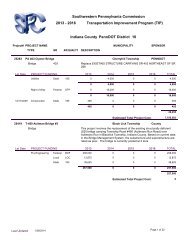
Major Traffic Flows 

Another factor that should be considered when 

considering intersection groupings is traffic 

flow demand paths. With an arterial, this 

issue is moot, but with a grid network, it can be 

crucial. With the grid pattern shown in the 

figure to the right, the horizontal dashed line 

shows a likely group boundary. However, 

when a major traffic flow pattern does a dogleg 

as shown at the bottom of this figure, then a 

different group boundary may be appropriate. 

This characteristic will probably manifest itself 

in the index, but when the signal engineer 

must make decisions based on sparse data, 

then knowledge of traffic flow patterns can be a 

useful discriminator to identify group 

boundaries. 

Coordinatability Factor 

There is one additional technique than can be employed by those that use the 

computer program, Synchro. Synchro has an internal methodology to calculate a 

“coordinatability factor”. This factor considers travel time, volume, distance, vehicle 

platoons, vehicle queuing, and natural cycle lengths. The coordinatability factor is 

similar to the “strength of attraction” but also considers the natural cycle length and 

vehicle queuing. The natural cycle length is defined as the cycle at which the 

intersection would run in an isolated mode or the minimum delay cycle length. The 

potential for vehicle queues exceeding the available storage is also considered in 

determining the desirability of coordination. 

Number of Timing Plans 

The “rule of thumb” for the number of signal timing plans is that each group requires a 

minimum of four plans: morning peak plan, average day plan, afternoon peak plan, and 

evening plan. But each signal group is unique and each group has unique demands. For 

example, an arterial that provides access to a regional shopping center may experience 

major demands on Saturday. Other examples abound of locations requiring other timing 

plans to meet demands by other major traffic generators like amusement parks, 

recreational demands, and other non-work related trips. 

One analytical method that can be used to estimate the need for a special timing plan is to 

plot the arterial traffic by direction by time of day. The plot of the sum of both directions 

provides an indication when cycle length changes may be required. Longer cycles are 

typically required to service heavier volumes. The ratio of one direction to the total traffic 

by time of day provides a good indication when offset changes may be required. The 

number of plans required and the time during which they will be used is needed in order to 

schedule the site surveys described in the next section. Analysis of the traffic demands at 

individual intersections will indicate when split changes are required. 

19

Cycle Length Issues 

As noted above, having a common cycle length is fundamental to coordinated signal 

operation. The cycle length must be evaluated from two different perspectives; individual 

intersection and the group cycle length. 

For the individual intersection, the recommended approach is to focus on the one or two 

major intersections in the group – the intersections with the highest demand because these 

intersections are the ones that will set the minimum cycle length limits. When evaluating 

cycle lengths, it is important to verify that the pedestrian timing is sufficient to allow 

pedestrians to cross the street. When the pedestrian timing is known, say 7 seconds Walk, 

10 seconds Pedestrian Clearance, and 3 seconds yellow change, and the vehicle phase is to 

be allocated at least 25 percent of the cycle, then the minimum cycle length that can meet 

both constraints is 20 seconds divided by 25%, or 80 seconds (assuming two critical phases). 

In general, the intersection in the group that requires the longest cycle length will set the 

group cycle length. The cycle length and splits can be determined by using either Webster’s 

equation or the Greenshields-Poisson Method. Both of these methods are explained below. 

In general, for a given demand condition, there is a cycle length that will provide the 

optimum two-way progression. This cycle length is a function of the speed of the traffic on 

the links between intersections and the link distance between intersections. This cycle 

length is called the “Resonant Cycle” and is explained further below. 

Webster’s Equation 

One approach to determining cycle lengths for an isolated pre-timed location is 

based on Webster's equation for minimum delay cycle lengths. The equation is as 

follows: 

Where: 

Cycle Length = (1.5 * L + 5) / (1.0 - Yi) 

L = The lost time per cycle in seconds 

Yi = Sum of the degree of saturation for all critical phases 5 

This method was developed by F. V. Webster of England’s Road Research 

Laboratory in the 1960’s. The research supporting this equation is based on 

measuring delay at a large number of intersections with different geometric designs 

and cycle lengths. These observations yielded the equation that is used today. It is 

important to recognize that this work assumed random arrivals and fixed-time 

operation – two conditions that can rarely be met in the United States. Notice that 

the equation becomes unstable at high levels of saturation and should not be used at 

locations where demand approaches capacity. Nevertheless, this technique provides 

a starting point when developing signal timings. To use this equation, 

5 

The critical phases are the ones that requires the most green time. The flow ratio is calculated by dividing the volume by the 

saturation flow rate for that movement. 

20

1. Estimate the lost time per cycle by multiplying the number of critical phases 

per cycle (2, 3, or 4) by 5 seconds (estimated yellow change plus red clearance 

time) to determine the “L” factor. L will have a value of 10, 15, or 20 and the 

numerator will equate to 20, 27.5, or 35 seconds. 

2. Estimate the degree of saturation for each critical phase by dividing the 

demand by the saturation flow (normally 1900 vehicles per hour per lane). 

3. Sum the degree of saturation for each critical phase and subtract the sum 

from 1.0. This is the denominator. 

4. To obtain the cycle length, round the division to the next highest five 

seconds. 

Greenshields-Poisson Method 

This approach to signal timing is statistically-based and makes several assumptions 

about the behavior of traffic. It uses the Poisson distribution to describe the arrival 

patterns of vehicles at an intersection. This distribution assumes that the vehicles 

travel randomly. This assumption is frequently a problem in urban areas, but like 

other methods, it can provide a good starting point to develop signal settings. 

While the Poisson distribution is used to estimate the arrivals, the time required for 

the approach discharge is based on work done by B. D. Greenshields in 1947. 

Surprisingly, this work has held up well during the intervening 50 years. Like 

Webster, Greenshields founded his work on many observations of traffic 

performance. The results of these studies are summed in the equation, 

Where: 

Phase Time = 3.8 + 2.1 * n 

Phase Time is the required duration to service the queue, and 

n is the number of vehicles in queue in the critical lane 6 . 

The basic procedure is iterative and uses the following steps. 

1. Assume a cycle length. For two critical phases, we suggest 60 seconds; for 

three critical phases we suggest 75 seconds, and for four critical phases we 

suggest 100 seconds. 

a. Calculate the number of cycles per hour by dividing 3600 (seconds per hour) 

by the assumed cycle length. 

2. For each critical phase, divide the demand volume by the number of lanes 

and by the number of cycles per hour to determine the mean arrival rate per 

lane. 

3. Use the Poisson distribution (Table 1) to convert the Mean Arrival Rate to 

the Maximum Expected Arrivals at the 95 Percentile level. 

4. Convert this Maximum Expected Arrivals to time required using 

Greenshields equation. 

6 The critical lane or movement for each phase, is the lane that requires the most green time. 

21

5. Add the time required for each critical phase plus the clearance and change 

time required (nominally 5 seconds) for each critical phase. If the sum is 

more than 5 seconds less than the assumed cycle, repeat the steps starting 

with the new (shorter) cycle length. If the sum is greater than the assumed 

cycle length by more than 5 seconds, repeat the steps but use the 90 th or 85 th 

percentile Maximum Expected Arrivals. If the calculations using the 85 th 

percentile arrivals indicate a cycle length greater than 80 seconds for twophase 

operation, 100 seconds for three critical phases and 120 seconds for 

four critical phases, then the volumes may be too high to use this method. 

Table 1 Poisson Distribution. 

Mean Arrival Rate 85 Percentile 90 Percentile 95 Percentile 

1 3 3 3 

2 4 4 5 

3 5 6 7 

4 7 7 8 

5 8 8 9 

6 9 10 11 

7 10 11 12 

8 11 12 13 

9 13 13 15 

10 14 15 16 

11 16 16 17 

12 16 17 18 

13 17 18 20 

14 18 19 21 

15 19 20 22 

16 21 22 23 

17 22 23 24 

18 23 24 26 

19 24 25 27 

20 25 26 28 

The Greenshields-Poisson Method is best suited to lower volume intersections. 

When the critical lane volume exceeds 400 vph then the basic assumption of random 

arrivals (no vehicle interactions) is probably not valid. Even within this range, care 

must be exercised. The method is designed to accommodate more vehicles than is 

expected on average; but some percentage of the time, 5% to 15%, the demand will 

exceed the time allocated and not all arrivals will be served. Care should be used to 

not apply this method at congested locations as the process will suggest 

unrealistically long cycle lengths which will result in high delay and long queues. 

Cycle Length 

When the traffic demand is balanced in both directions on the arterial, and when 

the distance between the intersections is approximately equal, then it is possible to 

obtain good progression in both directions by adjusting the cycle length using the 

following formulas: 

22

Where: 

(1) Cycle = 2 * Distance / Speed (1) 



Cycle is the cycle length in seconds, 

Distance is the link length in feet, and 

Speed is the average link speed in feet per second. 

These equations define resonant cycle lengths 7 for this signal group. Notice that the 

only real-time variable in the equations is traffic speed, which is actually used to 

estimate link travel time. This implies that different cycle lengths would be 

appropriate when there is a significant change in the link speed. It is typical for 

link speeds to be slower during the peak periods. This implies that it may be 

appropriate to use a longer cycle length during peak periods. 

Once an appropriate cycle length is selected using one of the three formulas noted 

above, the offsets can be identified as follows: 

With formula (1) -- the offset of an intersection at one end of the arterial is set to an 

arbitrary value – many engineers use 0 seconds. The offset at the next intersection 

is set to the sum of the value of the offset at the first intersection plus 50% of the 

cycle. For example if the offset of the first intersection is 0 and the cycle length is 

100 seconds, then the offset of the second intersection is 50 seconds. The offset of 

the third intersection and all other odd numbered intersections is the same s the 

offset at the first intersection, 0 seconds in the example. The offset at the fourth 

intersection and all other even numbered intersections is the same as the offset at 

the second intersection, 50 seconds in the example. This method of setting signal 

timing is called a Single Alternate and is the most desirable because it provides the 

maximum bandwidth in both directions. 

With formula (2) -- the offset of two intersections at one end of the arterial are set to 

an arbitrary value –0 seconds for example. The offset at the next two intersections 

are set to the sum of the value of the offset at the first intersection plus 50% of the 

cycle. For example if the offset of the first and second intersection is 0 and the cycle 

length is 100 seconds, then the offset of the third and fourth intersections is 50 

seconds. The offset of the fifth and sixth intersections is the same s the offset at the 

first and second intersection, 0 seconds in the example. The offset at the seventh 

and eighth intersection is the same as the offset at the third and fourth 

intersections, 50 seconds in the example. The offsets at additional intersections are 

in a similar manner. This method of setting signal timing is called a Double 

Alternate and is useful when the intersections are spaced more closely. It provides 

bandwidths half that provided by the Single Alternate solution. 

7 “Resonant Cycles in Traffic Signal Control”; Shelby, S.G.; Bullock, Darcy, and Gettman, Dougles; 

TRB Meeting, January 2005. 

23

With formula (3) -- the offsets at three intersections at one end of the arterial are set 

to an arbitrary value – 0 seconds for example. The offset at the next three 

intersections are set to the sum of the value of the offset at the first intersection plus 

50% of the cycle. For example if the offset of the first, second and third intersection 

is 0 and the cycle length is 100 seconds, then the offset of the fourth, fifth and sixth 

intersections is 50 seconds. The offset of the seventh, eighth, and ninth intersection 

is the same as the offset at the first, second and third intersection, 0 seconds in the 

example. The offsets at additional intersections set are in a similar manner in 

groups of three. This method of setting signal timing is called a Triple Alternate. 

This is appropriate for closely spaced intersections and provides a bandwidth onethird 

that of the Single Alternate. 

The important point to recognize when testing various Resonant Cycle lengths is 

that the speed of traffic is set based on what the average driver considers 

reasonable, not on an arbitrary speed that provides the maximum bandwidth. It is 

a common error to put a timing plan in the field that looks great on paper, but 

doesn’t work in the field because the vehicles are traveling faster (or slower) than 

the assumptions. Another related issue is that the average speed is not necessarily 

consistent throughout the day. It may be lower during the peak periods or at night, 

for example. Small errors in speed estimates can result in very poor signal timing 

(large offset errors), especially on suburban arterials where the distances between 

intersections are large. For example, estimating a speed of 30 MPH when in fact 

the true speed is 35 MPH will result in an offset error of 13 seconds on a 4,000 foot 

link. 

Offset Issues 

The offset is the heart of coordination signal timing. It is the difference in time from a 

reference point in the cycle at the upstream intersection to the same point in the cycle at 

the downstream intersection. This reference point is usually taken to be the beginning of 

the main street green. The simplest offset to consider is the one-way offset. When the light 

turns green at the upstream intersection and the platoon travels down the link, it is 

desirable for the downstream controller to change to green when the platoon approaches. 

This offset is appropriate for one-way streets and for situations when heavy demand in one 

direction justifies ignoring counter flowing traffic. 

Notice that this explanation deals with one link between intersections. Except at the ends 

of an arterial, the intersections on an arterial have one intersection upstream and another 

intersection downstream. It is important to recognize that changing the offset timing at 

one intersection affects the relative offset on four links. This is illustrated in Figure 2. 

24

Offset 

Figure 2. Offset change impacts. 

In this example the offset of the middle intersection is adjusted downward (earlier). Notice 

that this impacts the right-bound traffic flowing to the right intersection, as well as the two 

links of left-bound traffic. 

There is always a temptation to adjust the offset at one intersection to accommodate 

demand in one direction on one link without taking into account the effects of this change 

on the other three links. One way to manually analyze the offset impacts is to use the Kell 

Method described below. 

One-way Offset 

For the predominant one-way flow situation, the expedient approach requires only 

an estimate of the median travel time between intersections. The offset, expressed 

in seconds, is set at the intersections farthest upstream to an arbitrary value – many 

engineers use 0 seconds. The offset at the nearest downstream intersection is 

determined by adding the travel time to the offset of the adjacent upstream 

intersection. The travel time is estimated by dividing distance between the 

intersections by the average speed on the link. This process continues until the 

offsets of all intersections in the group have been determined. 

Notice that this method of determining offsets is independent of the splits at each 

intersection and the cycle length. 

As a further refinement, many traffic engineers will provide sufficient time for any 

standing queue to discharge before the arriving platoon. To do this, estimate the 

total number of vehicles in queue (vehicles that arrive during the red and do not 

turn right). Divide this number by the number of lanes, and multiply the result by 

2.5 seconds. Subtract this total from the offset that was determined by the link 

travel time. Adjusting for the average standing queue is referred to as the “Smooth 

Flow Offset.” As with the basic offset calculation method, when adjusting for the 

standing queues, start at the upstream intersection and work downstream 

calculating each offset based on the upstream offset by adding the travel time and 

subtracting the queue discharge time to the upstream offset at each intersection. 

25

Two-Way Offsets (Kell Method) 

The Kell Method is a technique that can be used to manually construct a Time-Space 

Diagram that results in balanced offsets in both directions. This technique is named 

after its developer; Mr. James H. Kell, who was an instructor at University of 

California, Berkley. The process is straightforward and requires a minimum of 

input information. An estimate of the percent green for the main street for each 

intersection, the average speed on the arterial, and the distance between 

intersections are the only information required to use the technique. The products 

of the method are the cycle length for the arterial and the offset for each intersection 

that provides equal bandwidth in each direction. 

1. Prepare a scale drawing laying out the intersections along the bottom of the 

page. 

2. Draw a vertical line at the first intersection on the left. 

3. Draw several cycles on the vertical line using a closed rectangle to represent 

the percent of time that the signal is NOT green. 

4. Draw a horizontal working line through the middle of either a green or not 

green 

5. Draw a line that slopes upward and to the right at the beginning of green at 

the left-most intersection. The sketch would something like that shown in 

Figure 3. 

Figure . Kell Method (Beginning) 

6. Plot the cycle of the next intersection such that either the green or the notgreen 

(whichever causes the beginning of green to come closest with the 

sloped line) is centered on the Working Line as shown in Figure 4. 

26

Figure . Kell Method (continued) 

7. Continue plotting the cycle for the remaining intersections by centering 

either the green or the red. A completed diagram is shown in Figure 5. 

Figure 5 . Kell Method (Completed Diagram). 

8. Notice that this technique forces a symmetrical solution that provides twoway 

progression with approximately equal bandwidths in each direction. The 

final step in the process is to determine the cycle length. In general, traffic 

will move on an arterial at a speed that the drivers consider reasonable for 

the prevailing conditions. The Engineer must estimate this speed and use it 

to determine the cycle length. Notice that the diagram shows that a vehicle 

requires approximately 1 ½ cycles to travel from intersection “A” to “D” in 

either direction. If the prevailing speed on the arterial were, 35 MPH, then 

an appropriate cycle length would be 75 seconds. This is determined by 

noting that it requires 1 ½ cycles to travel 5800 feet which is equivalent to 

3867 feet per cycle. The cycle length is determined by dividing the distance 

(3867 feet) by the speed, 51.33 ft/sec (35 MPH), and the cycle is 75 seconds. 

27

Split Issues 

The split is the amount of time allocated to each phase in a cycle at each intersection. The 

toolbox offers two ways to calculate splits manually, the Greenshields-Poisson method 

previously described and the Critical Movement method which is described below. 

Critical Movement Method 

This method uses techniques that were employed in the 1984 Highway Capacity 

Manual as a “Planning Analysis” (Figure 6) to estimate intersection capacity. We 

have adapted elements of this analysis to use to develop traffic signal timing 

parameters. To use this method, intersection turning movements, the signal 

phasing and the cycle length for the intersection must be known. The designer must 

determine the effective demand for each phase by applying various adjustment 

factors to reduce the demand to passenger car equivalents per lane (PCEPL). 

For the purposes of preparing traffic signal timing plans, a high level of precision is 

not needed. Traffic demand can vary plus or minus 20% in just a few minutes at a 

given location. Also a variation of 20% from day to day is not unusual. Our 

objective, therefore, is to develop timing plans that are robust and that will perform 

well through a wide range of demand conditions. The following steps are suggested: 

1. If the left turn movement is not protected, multiply the left turn demand by 

1.6. 

2. If the number of trucks is known, multiply the trucks by 1.5. 

3. Divide the traffic demand on 

the four major and left-turn 

approaches by the number of 

lanes for each movement. 

4. Determine the critical 

movements for both the east- 

west street and the north-south 

street. Determine the 

intersection critical movement 

by adding these two together. 

If this sum is less than 1500, 

then continue. If it is over 

1500 then the intersection is 

probably over saturated and 

the method may not be 

applicable. 

5. Determine the number of 

critical movements in each 

cycle. With no left-turn 

protection, there would be two, 

with left turn protection on one 

street there would be three, 

and with left turn protection on 

both streets there would be 

Figure 6. 

Example. 

Critial Lane Analysis 

28

four. Multiply the number of critical movements by five (the lost time) and 

subtract this number from the cycle length. This result is an estimate of the 

total available seconds of green per cycle that can be used for traffic 

movements. 

6. The final step is to multiply the total available green time by the ratio of the 

critical lane volume for the movement to the total intersection critical lane 

volume. For pre-timed operation, this is the phase green time in seconds. 

For coordinated operation with actuated controllers, this phase time is used 

to set the Force-off for the phase. For all actuated phases, the calculated 

time is the average green time for the phase. The phase maximum should be 

set at 25% to 50% greater than this value. 

29

IV. Local Controller Parameters 

It is useful to identify traffic signal timing parameters as being in one of two categories: 

local intersection timing parameters and coordinated operation timing parameters. The 

phase minimum or yellow change times are examples of local intersection timing 

parameters. The intersection cycle length and offset are examples of coordination timing 

parameters. There are far more local intersection timing parameters than coordination 

timing parameters. In fact, most systems define only three coordination timing 

parameters: cycle length, offset, and split. The following section of this report describe 

methods that can be used to set the local intersection timing parameters while the next 

section deals with the coordinated operation parameters. 

The basic timing parameters are essentially the same for all actuated controllers. There 

are subtle differences between different software implementations, for example, the NEMA 

controllers define the Force-off function as a “per ring” function while other 

implementations define the Force-off function as a “per phase” function. This distinction 

has little importance to the Traffic Engineer who is responsible for developing new Traffic 

Signal Plans. These differences, however, are very important when the results of a signal 

timing optimization process are implemented in a particular controller. Many newer 

controllers automatically calculate the force-off setting once the engineer defines the split. 

Because most jurisdictions use NEMA TS-1 and TS-2 or Model 170 actuated controllers, the 

primary emphasis has been placed on timing actuated controllers. It is important to 

recognize, however, that many jurisdictions use Pre-timed controllers. Most of the 

principles noted in this section can be directly applied to Pre-timed controllers. 

For the current status on signal timing, the reader is directed to Signal Timing Practices 

and Procedures: State of the Practice (Item IR-116) published by the Institute of 

Transportation Engineers. This report documents the current state-of-the-practice in 

traffic signal timing. It was prepared as part of a continuing program developed by FHWA 

and ITE to place increased emphasis on the quality of U.S. traffic signal timing. 

Actuated Controller Timing Principles 

Some of the basic principles of timing the green interval in a traffic actuated controller unit 

are as follows: 

 

 

 

Each phase must have a minimum green time so that a stopped vehicle that receives 

a green signal has enough time to get started and partially cross the intersection 

before the yellow signal appears. This time is sometimes called the initial portion of 

the green interval. 

Each vehicle requires enough green time to travel from the detector to the 

intersection. This is called passage time, vehicle extension, or gap. Gap refers to 

the distance between vehicles as well as the time between vehicles. Each successive 

vehicle actuation, therefore, increases the phase green time. With no opposing calls 

the controller rests. Extensions continue being timed, but with no effect on the 

green interval. 

There must be a maximum time that the green interval can be extended if opposing 

cars are waiting; this is called the Maximum Green or extension limit. 

30

Once an actuation is received from an opposing phase, the Maximum Green timer 

begins. The current phase will hold the green until the time between actuations is 

greater than the preset unit extension or gap. When a gap is detected, the yellow 

change interval will begin and the controller will transition to the next phase in 

sequence with demand. This is called termination by gap or gap-out. 

An actuation from another phase received during any portion of the green interval 

also starts the Maximum Green timing circuit. This is also called the extension 

limit. Even if actuations are close enough in time to prevent gap termination, the 

maximum limit will terminate the green interval when the preset maximum expires. 

This is called termination by maximum green or max-out. 

Basic Actuated Phase Settings 

All actuated controllers support these five basic, phase-timing parameters: 

Green, Extension, Maximum Green, Yellow and Red. 

Minimum 

Minimum Green (Initial) 

The Minimum Green is the first timed portion of the Green Interval. The duration 

of the Minimum Green is generally based on the number of vehicles that can be in 

queue between the upstream phase detector and the stop line. In general, the phase 

duration must be no shorter than some absolute minimum time, such as five to ten 

seconds. If pedestrians may be crossing with this phase, their crossing time must 

also be considered and included in the minimum phase length. 

The term, Minimum Green, is called Minimum Initial on some controllers. There is 

a subtle difference. The Minimum Green defines the duration of the green when 

there are no extensions. When the controller uses a Minimum Initial, the minimum 

green duration is equal to the sum of the Minimum Initial and one Extension. 

The minimum green time is the minimum assured green that will be displayed. It is 

established to allow vehicles that are stopped between the detector on the approach 

and the stop line to get started and move into the intersection. Therefore, timing of 

this interval depends on the location of the detector and the number of vehicles that 

can be stored between the detector and the stop line. 

Consideration must also be given to pedestrian timing. When there are no 

pedestrian provisions (indications or pushbuttons), the minimum assured green 

must be equal to the minimum pedestrian timing (walk + pedestrian clearance). 

One method that can be used to calculate the Minimum Green is: 

Minimum Green = 5 + 2n 

Where: 

“n” is the number of vehicles that can be stored between the stop line 

and the far detector in one lane. This is determined by dividing the 

distance (in feet) between the stop line and the detector by 25 since 25 

is the average vehicle length plus stopped-headway in feet. 

When stop-line detection is used, the Minimum Green can be quite short, say five to 

ten seconds. These very short minimums can be used on phases where there are no 

31

pedestrian movements, and on phases where there are actuated pedestrian signals. 

These extremely short minimums should never be used where there is the possibility 

of pedestrians crossing with the green display. 

Extension (Passage) 

The Extension (Passage) parameter extends the Green Interval for each vehicle 

actuation up to the Maximum Green. It begins timing when the vehicle actuation is 

removed; that is, when the vehicle passes over the detector. This extension period is 

subject to termination by the Maximum Extension timer or a Force Off. 

The actual Passage Time parameter (vehicle extension or gap time) is the time that 

the phase will be extended for each actuation. This setting is the number of seconds 

required for a vehicle moving at the approach speed to travel from the detector to 

the stop line. The passage time serves two purposes. (1) It is the passage time from 

the detector to the stop line and, (2) it is the allowable time gap between actuations 

that will cause the green to remain on that approach. As long as vehicle detections 

come at shorter intervals than the passage time (allowable gap), the green will be 

retained on that phase until the Maximum expires or it is Forced-off. 

If the passage interval is too short, quick stops may result as well as terminating the 

green before the vehicular movement has been adequately served. If the passage 

interval is set too long, excessive delays will result as well as safety problems due to 

improperly timed last vehicle intervals. 

Passage Time is calculated as follows: 

Passage Time = D / S 

Where: 

Maximum Green 

D is the distance from the stop line to the detector in feet; and, 

S is the speed on the approach in feet per second. 

This time setting defines the maximum length of time that a phase can be green in 

the presence of a conflicting call. If there is no conflicting call, it will be reset until 

an opposing call occurs. 

The Maximum Green timer is normally inhibited during coordinated operation when 

the phase maximum time is determined by the phase Force-offs. For most actuated 

phases, the Maximum Green should be considered a safety constraint, something to 

force the phase to end in the face of continuous demand. There is no accepted 

practice to determine the optimum setting. Some engineers feel that all phases 

should have similar limits like: 120 seconds for the primary through phases; 90 

seconds for the secondary through phases; and 60 seconds for the left-turn phases. 

Others set the phase maximums proportional to demand during a critical period. 

For example, one could calculate the phase splits using either the Critical Movement 

method then set the Maximum Green at 50% higher than the phase splits. 

32

Yellow 

The yellow interval follows the green interval at the end of each phase. The yellow 

interval is also referred to as the “change” interval and controls the duration of the 

yellow display for that phase. The phase change interval timing advises drivers that 

their phase has expired and they should: (1) come to a safe stop prior to the stop 

line, or (2) proceed through the intersection if they are too near the intersection to 

stop. 

The following equation is generally used to determine the proper change interval: 

Red 

Yellow Time = t + S / (2a +- 64.4 g) 

Where: 

t is the perception/reaction time of driver in seconds (typically 1.0 

second). 


a is the deceleration rate in feet per second (typically taken as 10 feet 

per second squared) 

g = approach grade, percent of grade divided by 100 (add for up-grade 

and subtract for downgrade) 

The red clearance interval (also known as the all-red interval) follows the yellow 

interval of each phase. It must expire before the next phase in sequence can begin. 

It is normally one to two seconds but on slower speed approaches, it is not unusual 

to use a very short duration of 0.0 to 0.5 seconds since the Yellow time of 3.0 to 4.0 

seconds provides sufficient time to meet both the change and the clearance 

requirements. 

Red Time = (W + L) / S 

Where: 

W is the Width of intersection in feet 

L is the length of vehicle in feet (typically taken as 20 feet) 


Pedestrian Parameters 

There are two pedestrian timing parameters, Walk and Flashing Don’t Walk (pedestrian 

clearance. Where pedestrian movements regularly occur, pedestrians should be provided 

with sufficient time to cross the roadway (MUTCD section 4D.03). In other words, unless 

the pedestrian movement is actuated, the time required for pedestrians to safely cross the 

road (the sum of the Walk and Don’t Walk times) will dictate the minimum green time for 

that phase. When pedestrian pushbutton (actuation) is provided, then the normal vehicle 

minimums would be used in the absence of a pedestrian actuation. Notice that it is possible 

33

to have a signal design that uses pedestrian pushbutton detection without using pedestrian 

Walk and Don’t Walk displays. 

Walk 

The Walk parameter controls the length of time that the walk signal is displayed. 

Under normal conditions, the walk interval is 4 to 7 seconds. This allows 

pedestrians to have adequate opportunity to leave the curb before the clearance 

interval is shown. Under special circumstances, such as at a school crossing with 

numerous pedestrians, walk times may exceed 7 seconds. Research indicated that 

pedestrian queues of 24 or more people can be accommodated in 7 seconds. 

Flashing Don’t Walk 

The pedestrian clearance parameter controls the duration that the Flashing Don’t 

Walk is displayed. This is the time required for a pedestrian crossing in the 

crosswalk to leave the curb and travel out of the traveled way (MUTCD section 

4E.02) before opposing vehicles receive a green indication. 

The Flashing Don’t Walk (pedestrian clearance) is calculated as follows: 

Flashing Don’t Walk = W / SP 

Where: 

Volume-Density Phase Settings 

W is the walking (crossing) distance in feet from curb to curb; and, 

SP is the average walking speed in feet/sec (typically 3.5 to 4 feet/sec). 

In the 1950’s the Automatic Signal Company introduced two new and complex traffic signal 

controllers, the Model 1022 and the Model 1033. These controllers had far more timing 

circuits than any controllers used before or since. Although all of the timing parameters 

were well-founded in theory; in practice, many did not actually improve the performance of 

the intersection. There were several reasons for this experience: it was not possible to 

determine which of the many timers actually caused a particular phase to terminate, the 

analog timing circuit technology available at the time was subject to variations based on 

temperature and humidity, and like today, few engineers had the time necessary to finetune 

the operation. Of the many features of these innovative controllers, two features, 

variable initial and gap reduction, have evolved and are typically available with today’s 

controllers. These two features are explained below. 

Variable Initial 

To successfully employ the volume density features of a controller, it is necessary to 

have phase detection farther upstream than that which is normal. This enables the 

controller to sample traffic on the approach with a minimum impact from a standing 

queue. Detection 300 to 400 feet upstream from the stop line is typical with volume 

density operation. With detection this far back, the Minimum Green would be quite 

long – 35 seconds with the detector back 400 feet. Since a Minimum Green this long 

would result in very sluggish operation when the demand is light, two other timing 

circuits are used to mitigate these impacts: Variable Initial and Maximum Initial. 

34

Added Initial – This interval times concurrently with the minimum green interval. 

The value is the amount of time that is added when each vehicle actuation is 

received during the initial period. The actual minimum green time used by the 

controller is the greater of the minimum green or the added initial sum. The Added 

Initial cannot exceed the Maximum Initial. The Added Initial allows the duration of 

the Minimum to vary between the actual minimum and the time required to 

discharge the maximum queue that can be stored between the stop line and the 

detector. 

Maximum Initial – This is the maximum period of time for which the Added Initial 

can extend the initial green period. The Maximum Initial can not be less than the 

Minimum Green. 

Gap Reduction 

Gap Reduction is the other legacy concept that is used on the modern controller. 

This parameter is used to allow the “gap seeking” logic of the actuated controller to 

identify a smaller gap in traffic to justify terminating the phase than that which is 

implied by the Passage Time. Gap Reduction is a means of reducing the passage 

time or gap on the basis of the time that opposing vehicles have waited. In effect, it 

benefits the waiting vehicles by reducing the time allowed between vehicles arriving 

on the green phase before that phase is terminated. There are three timing 

parameters associated with the Gap Reduction feature: Time-Before-Reduction, 

Time-to-Reduce, and Minimum Gap. 

Time-Before-Reduction – This period begins when the phase is Green and there is 

a serviceable call on a conflicting phase. When this period is completed, the linear 

reduction of the Passage Time begins. 

Time-To-Reduce – This period begins when the Time-Before-Reduction ends and 

controls the linear rate of reduction until the Gap is reduced to the Minimum Gap. 

Minimum Gap – Like the Passage Time, this parameter extends the Green Interval 

by the Minimum Gap time for each vehicle actuation up to the Maximum Green. It 

begins timing when the vehicle actuation is removed. This extension period is 

subject to termination by the Maximum Green or a Force Off. 

Controller Timing Parameters Summary 

There are 12 controller timing parameters that are commonly used: 

1. WALK Establishes the length of the WALK interval. 

2. PED CLEARANCE Establishes the length of flashing DON’T WALK 

interval. 

3. MINIMUM GREEN Establishes the length of initial state of green interval. 

4. PASSAGE TIME Establishes the increment of right of way (green) time 

extension for each vehicle actuation during the green 

interval. 

35

5. MAXIMUM GREEN Establishes the maximum limit to which the green 

interval can be extended on a phase in the present of a 

serviceable demand on a conflicting phase. 

6. ADDED INITIAL Density feature. Establishes number of seconds by 

which each vehicle (actuation) increases the initial state 

of green during non-green time on the phase 

7. MAXIMUM INITIAL Density feature. Establishes the maximum limit to 

which the initial interval can be extended on a phase. 

8. TIME B4 REDUCTION Density feature. Establishes a preset time before the 

allowed gap (Passage Time) begins to reduce. 

9. TIME TO REDUCE Density feature. Establishes time in which the allowed 

gap is reduced from passage time to minimum gap, after 

the time before reduction has expired. 

10. MINIMUM GAP Density feature. Establishes minimum value to which 

allowed gap between actuations on phase with green can 

be reduced upon expiration of time to reduce. 

11. YELLOW CHANGE Establishes the length of yellow interval following the 

green interval. 

12. RED CLEARANCE Establishes the length of red clearance interval following 

the yellow interval. 

36

V. Coordination Timing Issues 

There are three parameters that determine how a controller functions in a coordination 

mode: cycle length, offset, and split. While all three parameters are important to the 

efficient operation of a signalized arterial or network, it might be argued that the cycle 

length is the most important of these parameters because it is the cycle length that 

determines the periodicity of the system. 

Resonant Cycle 

In the discussion of the cycle length, we introduce the concept of the resonant cycle length 8 . 

That is, for regular linear and grid networks, there are one, two, and sometimes three cycle 

lengths that provide much better operation than other cycles. In other words, the concept 

of a resonant cycle is a cycle length that accommodates good two-way progression. The 

resonance (and non-resonance) of a cycle time stems from the principle that intersection 

spacing precludes good progression at certain cycle lengths, and conversely some cycle 

lengths necessarily preclude progression on an arterial due to their incompatibility to the 

network geometry. The second essential element of a resonant cycle is that it continues to 

provide good two-way arterial progression over a range of volumes. 

Resonant cycles naturally arise on arterials as a function of what cycle provides good twoway 

progression for given intersection spacing, vehicle speeds, volume levels, saturation 

flow rates, and phase sequencing. Time-space diagrams, can be used to provide a 

convenient means of conveying the traffic flow mechanics that give rise to the resonant 

cycle. The results of the experiments, taken as a whole, suggest that well-chosen cycle 

lengths scheduled by time-of-day or selected from a table dynamically could yield better 

progression, delay, and travel time performance than an on-line incremental adjustment 

strategy based on maintaining a constant, target degree of saturation for the single most 

congested intersection – a typical adaptive control strategy. 

Optimizing an arterial signal-timing plan (cycle, splits, and offsets) for a singular set of 

input volumes can be handled in a straightforward manner by using signal-timing 

optimization software such as TRANSYT-7F or Synchro. However, a much more 

challenging task is compiling a set of Time of Day (TOD) signal-timing plans and a TOD 

schedule for each day of the week, in order to accommodate all hourly and daily fluctuations 

in traffic conditions typically experienced during the week. 

There are currently no commercially available off-the-shelf tools to address this problem 

and even the literature offers very little in terms of structured guidance to accomplish this 

task. The decisions to be made include the following: 

 

Select a workable number of plans. For example, fifteen signal-timing plans usually 

are not practical. A typical day might minimally consist of four plans: the AM peak, 

the PM peak, and off-peak Day and Night conditions. Also for areas in the vicinity 

of major shopping facilities one might consider a special plan to accommodate 

shopping traffic demand. 

8 “Resonant Cycles in Traffic Signal Control”; Shelby, S.G.; Bullock, Darcy, and Gettman, Dougles; 

TRB Meeting, January 2005. 

37

Construct a schedule. Each hour of the week must be covered by a signal-timing 

plan. For example, the schedule determines when the AM peak plan starts and ends, 

subsequently switching to the off-peak plan. 

Determine the input volumes to generate each plan. Over the hours each signaltiming 

plan will be in operation, traffic conditions may fluctuate significantly. 

However, signal-timing optimization software only accepts a single set of input 

volumes to generate a corresponding plan. For example, a user might use the peakhour 

flows observed over the whole time frame a plan will be in effect. 

The decisions are all interrelated. For example, the number of workable plans may depend 

on the number of “distinct” traffic conditions that can be discerned. The construction of the 

schedule will depend on the number of timing plans that are appropriate through a given 

day. The input volumes will depend on what time of day a plan is in effect. Until very 

recent publications, engineering judgment was the only guide to making these decisions. 

A paper 9 published in 2002 suggests that a statistical clustering algorithm, based on 

volumes approach the arterial’s critical intersection be used to determine “break-points” (or 

switch points) between TOD plans in the daily schedule. 

A subsequent paper 10 , published in 2004, suggested flaws with using volume clusters, and 

suggested that instead, 90th percentile volumes (of a set of several TOD observations) of 

the critical intersection be used to optimize its cycle length based on a uniform delay 

equation. These plans would then be evaluated over several TOD intervals (using a genetic 

algorithm) to optimize the TOD schedule of the critical intersection. 

Intersection Categories 

In the signal network to be retimed, all intersections can be divided into two categories: 

primary intersections and secondary intersections. The primary intersections are the ones 

that have the highest demand to capacity ratio and will therefore require the longest cycles. 

These intersections are usually well-known to the Traffic Engineer. They are the 

intersection of two arterials, the intersections with the worst accident experience, the 

intersections that service the major shopping centers, the intersections that generate the 

most complaints. The secondary intersections are the ones that generally serve the 

adjacent residential areas and local commercial areas. They are usually characterized by 

heavy demand on the two major approaches and much less demand on the cross street 

approaches. 

The purpose of assigning intersections to one of these two categories is to reduce the 

locations where traffic counts are required. The primary intersections require turning 

movement traffic counts – there is simply no other way to measure demand. However, the 

9 

Smith, B. L., W. T. Scherer, T. A. Hauser and B. Park, “Data-Driven Methodology for Signal Timing Plan 

Development: A Computational Approach”. Computer-Aided Civil and Infrastructure Engineering, Vol. 17, 

2002, pp. 287-395. 

10 

Park, B., Santra, P., Yun, I., Lee, D., Optimization of Time-of-Day Breakpoints for Better Traffic Signal 

Control. In TRB 83rd Annual Meeting Compendium of Papers. CD-ROM. Transportation Research Board, 

National Research Council, Washington, D.C., 2004. 

38

secondary intersections usually have side street demand that can be met with phase 

minimum green times. The strategy, therefore, is to concentrate the counting resources at 

the locations where there is no substitute, and to use minimum green times for the minor 

phases at secondary intersections. 

Number of Timing Plans 

A unique timing plan is required whenever a cycle length, offset, or split is different from 

the previous setting. When a new timing plan is selected, the controller must “transition” 

to the new plan. During this transition period, systematic operation in the network is 

interrupted while each controller adjusts to the new parameters. Because of this 

disruption, transitions are minimized and one must be assured that the benefits of the new 

plan overcome the disbenefits of the transition period. 

One way to determine how many timing plans are needed is to assume that a new plan is 

needed whenever there is a significant change in the traffic demand. This may be assessed 

by evaluating the changes in demand by hour by direction. For the network, array the 

northbound, southbound, eastbound and westbound in a table where the directional flows 

are in columns and the rows represent the hourly data. Let a column of the table represent 

the sum of the four directional flows. Examine this column to identify the time during 

which there is a significant change in the total demand, this is an indication that different 

cycle length (new timing plan) may be warranted. 

Assuming that the major flows are on the north-south street, calculate the basic split by 

dividing the greater of the northbound or southbound by the total intersection demand for 

the period. When this ratio changes is a good indication of the need for a new plan to 

accommodate a new offset. Periods when a new plan may be warranted are identified by 

the changes in either the total demand or the split demand. 

Using the Tool Box 

We have placed a significant emphasis on discussing resonant cycle lengths because plan 

changes involving different cycle lengths are very disruptive during the transition period. 

In contrast, timing plan changes that involve different offsets with the same cycle length 

are relatively benign, and plan changes that only involve split differences are generally 

unnoticed. It is important therefore, to identify the resonant cycle and use this cycle for as 

many plans as possible. 

When a computer model is not available, we suggest that the following procedure be 

followed: 

1. Cycle - For each Primary intersection, calculate the Cycle Length required using 

Webster’s equation as defined in Section 4.1. For each signal group, determine the 

Resonant Cycle Length using the equations provided in Section 4.2. Select the 

longest Cycle for the timing plan. 

2. Split - For each Primary intersection determine the intersection splits using the 

Critical Movement Method explained in Section 4.5 and the selected Cycle. For each 

Secondary intersection, determine the time required for each minor movement using 

the Greenshields-Poisson Method and the Cycle explained in Section 4.6. Check 

39

oth Primary and Secondary intersections for pedestrian timing requirements and 

adjust as necessary. 

The purpose of obtaining count data is to use it as input to a timing model. The 

timing model then generates the appropriate signal settings. There is an alternative 

way, and that is to estimate the settings directly. This is what we are doing when 

we estimate the minimum phase time for the cross street movements at a Secondary 

intersection. The turning movement data at the primary intersection might show 

that the cycle length for the group should be 100 seconds. If we allow a phase 

minimum of ten seconds and assume five seconds for the change and clearance 

intervals, then we can determine that the side street split should be 15%. To work 

the numbers another way, there will be 36 100-second cycles per hour. Ten seconds 

is sufficient time to discharge three to four vehicles per cycle. In other words, this 

strategy will provide enough capacity to discharge approximately 125 vehicles per 

lane in an hour. As long as the demand is less than the 125 vehicles per lane, this 

approach will work fine. 

This example describes one way to estimate secondary intersection split, given the 

cycle length. For system timing, we must also have a means of estimating the third 

parameter, the offset. We can do this for two conditions, when the demand in one 

direction is predominant and when the demand is relatively balanced. 

3. Offset - Determine the offsets using the Kell Method as outlined in Section 4.4. 

When using the Kell Method (or any maximum bandwidth method) the Practitioner 

has several options. The most obvious, and most frequently used, is to consider an 

arterial as single entity. This will generally result in balanced bandwidths in both 

directions. 

During periods of directional flow, however, it may be useful to consider a minor 

variation. Within any arterial group, the signals can be clustered in subgroups. The 

intent is to cluster signals that have similar link lengths into subgroups. The Kell 

Method is then applied to each cluster which by virtue of the similar link lengths 

will have good progression in each direction. The offsets within the subgroups are 

those generated by the Kell Method. The offset between clusters is set using the 

One-way Method defined in Section 4.3 to favor the peak directional movement. 

This technique assures good progression in the peak direction while providing good 

progression within the clusters in the counter flow direction. 

During periods of heavy directional flow, it may be necessary to ignore the contra 

flow traffic in order to accommodate the peak directional demand. In this instance, 

all of the offsets are developed using the One-way Method as described in 

Section 4.3. 

40

VI. Signal Timing Examples 

One way to illustrate how the tools and techniques presented in this document can be used 

to develop good signal timing plans on a shoestring (low budget) is to provide an example. 

Three different examples are discussed illustrating different measures that could be used 

depending on the available resources. 

Moderate Signal Timing Budget 

In this example, the agency retained a consultant to prepare signal timing plans for a 

suburban arterial three years ago when the arterial was widened and new controller were 

installed. The new timing plans worked well in the beginning, but as development 

increased in the corridor, some obvious problems are beginning to emerge. Most of the 

problems can be related to the opening of the new shopping center with major signalized 

entrances at two of the ten signals in the corridor. Although a consultant prepared the 

existing signal timing plans, the agency required the consultant to develop the timing plans 

using the same program that the agency uses and required the consultant to deliver all of 

the data input files for the program. 


In the example, this is obviously the ten intersections described in the arterial. 


This is a critical step in minimizing the cost of developing new plans. In the 

example, one can assume that there are turning movement counts available for all 

ten intersections – the only problem is that they are three years old and there have 

been changes in the traffic demand in the corridor. Nevertheless, it is likely that 

some of the existing turning movement data can be updated and used in developing 

the new plans. It is likely, however, that new turning movement counts will be 

required for the two intersections that are the entrances to the shopping center. 

Another type of data that will prove to be very useful is a 24-hour directional count 

on the arterial. The directional count can be used to estimate any overall change in 

the traffic demand during the last three years. Factors developed using these data 

can be used to adjust the three year old turning movement counts to reflect the 

current demand. 

The agency is fortunate in that other data that would normally be collected: distance 

between intersections, intersection geometry, signal phasing, and the like is already 

available and coded in the optimization program input files. For the most part, the 

agency only has to update the traffic demand information and rerun the program to 

obtain updated signal timing plans. 


Although many engineers are tempted to skip this step, experience has shown that a 

visit to the site during the hours for which the timing plans are being developed can 

be very beneficial. 

41

Specific things to look for are unusual demand conditions. In the example, the 

timing at the two intersections affected by the shopping center needs to be updated, 

one might assume that the signal settings at the other eight intersections may be 

pretty good. This can be confirmed by a quick trip to the location during the peak 

periods. This field visit frequently exposes additional issues that can be readily 

addressed with new timing plans. 


This is the key step in minimizing the cost of developing signal timing plans. In the 

example, assuming that the 24-hour data can be used to update the old turning 

movement counts and assuming that the site visit did not uncover a latent demand 

condition, new counts would be needed only at the two intersections that are heavily 

impacted by the shopping center. The 24-hour directional count data is used to 

reaffirm that the arterial should continue to operate with four timing plans. 

To obtain the turning movement data, the agency will conduct short counts during 

the AM Peak, PM Peak, afternoon, and evening periods at the two locations. The 

times when the short counts are scheduled are determined from the 24-hour 

directional data. Factors developed from the 24-hour directional data are used to 

update the existing turning movement counts at the remaining eight intersections. 


Because there is no significant change proposed to the operation of the individual 

controller, there is no need to change any of the local timing parameters. 


Because there is no need to change the structure of the system, there are no changes 

required in the grouping of the signals. 


Once the turning movement data are available, it is a simple matter to update the 

input files and to rerun the optimization program. 


The physical installation of the new timing plan parameters is usually a 

straightforward, but a task that is done manually offers the potential for significant 

errors. A major concern in the installation phase is to verify that the optimized 

parameters are in fact, the parameters that are installed. 

The second issue in this step is to evaluate how effective the new settings are. For 

agencies that have some resources that can be applied to signal timing issues, 

evaluation is an area that provides increasing benefits over time. To evaluate the 

timing plans developed in this scenario, two separate types of studies are 

recommended: travel time and stopped-time delay. The travel time studies a route 

up and down the arterial will provide a quantifiable measure of the traffic 

performance in the corridor. To compliment this information, delay studies at 

selected intersections will provide insight to the operation of specific intersections. 

In the example, consider making delay studies at the two intersections where 

entirely new plans were installed. In addition, it is appropriate to make delay 

42

studies at the critical intersection in the group. The critical intersection is generally 

the most congested; it is the intersection that drives the cycle length for the group. 

The combination of travel time studies and delay studies will provide an excellent 

baseline condition against which future changes in signal timing can be compared. 

Modest Signal Timing Budget 

The second example uses a similar geometric situation with an entirely different system 

history. In this case, there is a ten intersection arterial; but until now, all intersections 

have operated as full-actuated, isolated signals. The agency has just hired an electrical 

contractor to install new controllers, interconnect cable, and an on-street master. This is 

the classical installation of a “closed loop” system. To save scarce funding, the agency plans 

to develop the timing plans themselves and has limited resources for this effort. 


In this second example, it is obvious that the ten intersections will constitute the 

signal system. 


The use of existing data is even more critical in minimizing the cost of developing 

new plans. In this example, one can assume that there are turning movement 

counts available for all ten intersections; but the turning movement counts were 

made during different years. Some of the existing counts are more than ten years 

old. While there have been changes in the traffic demand in the corridor over the 

last ten years, most of the development has taken place on the East side. It is likely 

that some of the existing turning movement data at intersections on the West side 

can be updated and used for developing the new plans. It is likely, however, that 

new turning movement data will be required for the five intersections on the East 

side. 

As with the first example, the 24-hour directional count on the arterial will prove to 

be very useful. If a recent directional count is not available, one must be made as a 

first step. Hopefully, there are older 24-hour counts that are available and can be 

used to develop factors that can be used to adjust the existing turning movement 

counts to reflect the current demand. 

Although the available funds are modest, the agency owns a signal timing 

optimization program and plans to use it. This decision may cost a little more in the 

short run, but it will allow the agency to easily revise the signal timing plans in the 

future when the input file is updated with new turning movement counts. In the 

meantime it is necessary to collect all of the descriptive required by the program. 

This descriptive data includes the following: 

 

A condition diagram of each intersection showing the number of lanes and 

width of each lane on all approaches. The condition diagram must have a 

North arrow and show the street names. 

43

A phasing diagram for intersections with existing controllers. It is important 

for the phasing diagram to include the NEMA phase number for each phase 

movement. The phasing diagram must also show all overlaps (if any). 

Distance between intersections and the free-flow travel speed for the 

conditions under which the timing plan will operate. This information should 

be depicted of a map of the area showing the roads and signalized 

intersections. It is not necessary for the map to be drawn to scale, it is 

important for each link on the map to be long enough to be able to show 

various data such as link length, speeds, and volume. 

With this information in hand, particularly the 24-hour directional count, the 

Engineer can begin making some difficult decisions concerning turning movement 

data. A first step is to identify each intersection as either a Primary or Secondary 

intersection. As previously noted, the Primary intersections are the ones that are 

the most congested and are the intersections that drive the cycle length 

requirements. Another initial step is to determine how many timing plans are 

required for the facility. Using the methodology that compares total intersection 

and directional volume hour by hour is a good indication of when new timing plans 

are needed. 

The Engineer has three options to obtain the turning movement data that is 

necessary to run the optimization program: update the existing counts, make new 

counts using short-count techniques, or estimate the turning movements using a 

program like Dowling Associates’ “TurnsW”. With the provided scenario, one would 

tend to update the intersections on the West side (lowest growth) and make new 

short counts at the intersections on the East side. The estimated counts could be 

used at Secondary intersections on the West side if data collection costs were a 

major limitation. 


To save time and cost, many engineers are tempted to skip this step. This would be 

a mistake. Experience has shown that a visit to the site during the hours for which 

the timing plans are being developed will be beneficial. 


This is typically the most costly step in the signal timing process. After making the 

best possible use of the existing data as previously described, this step provides for 

the field data collection of turning movement counts. 


Because the existing controllers are operating in the full actuated mode, the local 

timing parameters probably do not require any change. 




44


Once the turning movement data are available, it is possible to run the optimization 

program. 


The physical installation of the new timing plan parameters is usually 

straightforward, but any task that is done manually offers the potential for 

significant errors. A major concern in the installation phase is to verify that the 

optimized parameters are in fact, the parameters that are installed. 

The second issue in this step is to evaluate how effective the new settings are. For 

agencies that have few resources the evaluation must frequently be subjective. 

Nevertheless, this element is a very important part of the signal timing process. 

Rather than conducting formal travel time studies, the Engineer may simply drive 

the arterial several times looking for discontinuities in the traffic flow or congestion 

where none was expected. These informal evaluations must be conducted during the 

periods for which the timing plans were developed. The Engineer should pay 

particular attention to any instances of cycle failure (approach demand is not met 

during a green phase) as an indication of a serious deficiency. 

Minimum Signal Timing Budget 

The third example involves developing signal timing with the absolute minimum of 

resources. This example is similar to the previous example, except there are only five 

intersections on the arterial and all are currently operating as isolated, actuated 

controllers; but the controllers have time-base coordination capability and the Engineer 

wants to use this function. 

In the previous examples, the cost of preparing the plans was minimized by minimizing the 

cost of the data collection effort necessary to run the optimization software, specifically the 

turning movement counts. With this absolutely minimalist approach, a different approach 

is used. Instead of estimating the input data, the process involves estimating the 

parameters (cycle length, split, and offset) themselves using time-space geometry and 

estimates based on engineering judgment. 


In the example, the system consists of the five intersections. 


As with the previous examples, the Practitioner must make maximum use of 

existing data, especially existing timing data and system layout information. 


This step is absolutely vital with the minimalist approach. The Practitioner must 

carefully observe each of the five intersections for several cycles during the period 

for which the timing plan is being developed. In this survey, the Practitioner must 

estimate the average speed of the traffic between intersections on the artery; and if 

not available in the existing data, the Practitioner must measure the distance 

between intersections. 

45

As with the previous examples, specific things to look for are unusual demand 

conditions, pedestrian demands, and any congested movements. The primary 

output of this effort is the identification of the Primary intersection in the group. 


With the minimalist approach, the Practitioner must obtain current turning 

movement information for the Primary intersection usually by using short count 

techniques as with the previous examples. In addition, the Practitioner must obtain 

24-hour directional counts on each of the four major approaches to the Primary 

intersection. 

At Secondary intersections, the Practitioner must observer the operation of the 

intersection for several cycles and record the average phase time for each phase 

during the cycle. 


Unless a problem is identified during the Site Survey, there is usually no need to 

change any of the local timing parameters. 





In the previous two examples, this step involved running an optimization program. 

With the minimalist approach, this step involves estimating the coordination 

parameters directly. 

Cycle Length – The cycle length must be selected for the group based on meeting 

three criteria; optimum cycle length, resonant cycle length, and pedestrian 

constraints. 

Using the turning movement information at the Primary intersection, calculate the 

optimum cycle length using Webster’s equation: 

Cycle Length = (1.5 * L + 5) / (1.0 - Yi). 

Using the intersection layout and phasing, determine the minimum pedestrian cycle 

length: 

Ped Minimum Cycle = LT + 14 + Wm / SP + Wc / SP + Y 

Where: 

LT = Time required for the left turn movements. 

14 = (2 * 7) Time that the “Walk” is displayed to cross each street. 

Wm / SP = Width of the Main Street divided by the pedestrian speed. 

Wc / SP = Width of the Cross Street divided by the pedestrian speed. 

Y = Yellow and All Red time for critical phases. 

46

Using the average distance between the five intersections, calculate the potential 

resonant cycles using the following equations: 

Cycle = 2 * Distance / Speed, 

Cycle = 4 * Distance / Speed, 

Cycle = 6 * Distance / Speed. 

Cycle = 8 * Distance / Speed. 

Select the shortest resonant cycle which is longer than the optimum cycle and the 

pedestrian minimum cycle. If none of the resonant cycles are longer than the 

optimum cycle, select the longest resonant cycle. 

Offset – The offset is calculated using the Kell method. 

Split – The split is calculated for the Primary intersection using the Critical 

Movement Method. Once the splits are calculated based on demand, they must be 

checked to verify that the pedestrian requirements are met. For example, assume 

that the calculated splits required 15 seconds for phases 4 and 8. If the minimum 

pedestrian time were 19 (7 + 48/4) seconds, then the intersection split would have to 

be increased to 19 seconds to accommodate the pedestrian movement. 

At intersections other than the Primary intersection, the split is based the average 

phase time observations. These averages are converted to a percent of the cycle and 

new splits are calculated by multiplying these percent splits by the new cycle length. 

The final split is based on the pedestrian requirement or the average phase time, 

whichever is longer. 


As with the other methods, the physical installation of the new timing plan 

parameters is usually straightforward, but any task that is done manually offers the 

potential for significant errors. A major concern in the installation phase is to verify 

that the optimized parameters are in fact, the parameters that are installed. 

This minimalist approach takes many short cuts compared to the steps that would 

be followed in a traditional signal timing effort. It is very important for the 

Practitioners to carefully verify these plans in the field. In fact, in spite of the 

objective of minimizing costs, more time and effort should be planned for this task 

under this approach than either of the two other approaches that use optimization 

software. It is recommended that the new plans be tested during a period of low 

traffic demand conditions before they are used in the period for which they are 

designed. For example, a plan for the AM rush hour might be tested in the late 

morning or early evening when the demand is usually lighter. This test period 

should allow the Practitioner to identify any serious discrepancies without having a 

large negative impact on traffic operations. 

47

U.S. Department of Transportation 

Federal Highway Administration 

Office of Operations 

400 7 th Street S.W. (HOP) 

Washington, DC 20590 

Publication No. FHWA-HOP-05-034 

48

FHA Signal Timing On A Shoestring

You also want an ePaper? Increase the reach of your titles

Delete template?

Save as template?