Analysis of Noise â Part V - Spectroscopy

More documents

Recommendations

Info

........................... CHEMOMETRICS IN SPECTROSCOPY ............................ small compared with the reference signal, and therefore the signalto-noise ratio (S/N) was high. We then noted that if that condition did not hold for any particular set of measurements, then other phenomena also come into action. We pointed out that under low-noise conditions the signal can affect the noise level, but under conditions in which the signal is weak or the noise excessive, the noise can affect the computed transmittance as well. The expressions we obtained showed that as the reference signal gets weaker and weaker (or the noise gets larger and larger), the system first reaches a point at which the expected value of T is larger than E s /E r , and as the reference signal continues to decrease, the multiplying factor first goes through a maximum and then decreases so that the expected value of T approaches zero as the reference signal energy, E r , approaches zero. We are now ready to consider the behavior of the noise under conditions in which it is not small compared with the signal. We start with the definition of transmittance, as we pointed out previously, and we rewrite the equation here: T E s /E r [6] To put equation 6 into a usable form under the conditions we wish to consider, we could start from any of several points of view: the statistical approach of Hald (11), for example, which starts from fundamental probabilistic considerations and also derives confidence intervals (albeit for various special cases only); the mathematical approach (12) or the Propagation of Uncertainties approach of Ingle and Crouch (13). Inasmuch as any of these starting points will arrive at the same result when done properly, the choice of how to attack an equation such as equation 6 is a matter of familiarity, simplicity, and, to some extent, taste. We, being chemists and spectroscopists, and writing for spectroscopists, will use the Propagation of Uncertainties approach of Ingle and Crouch: [64] Note that we use the letters C,D to represent the variables in equation 64 to avoid confusion with our usage of A to mean absorbance. 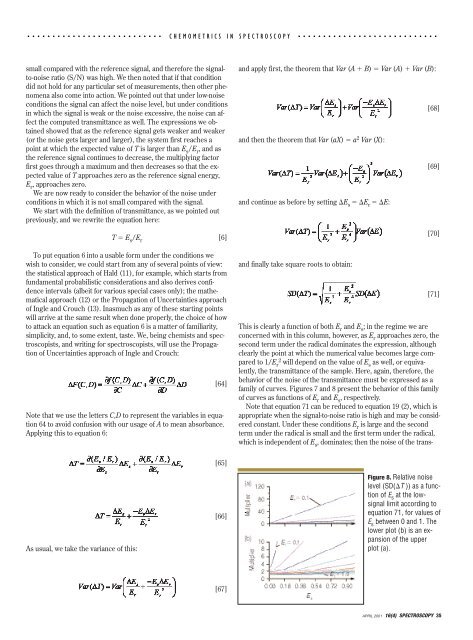Applying this to equation 6: and apply first, the theorem that Var (A B) Var (A) Var (B): and then the theorem that Var (aX) a 2 Var (X): and continue as before by setting E s E r E: and finally take square roots to obtain: [68] [69] [70] [71] This is clearly a function of both E r and E s ; in the regime we are concerned with in this column, however, as E r approaches zero, the second term under the radical dominates the expression, although clearly the point at which the numerical value becomes large compared to 1/E r 2 will depend on the value of E s as well, or equivalently, the transmittance of the sample. Here, again, therefore, the behavior of the noise of the transmittance must be expressed as a family of curves. Figures 7 and 8 present the behavior of this family of curves as functions of E r and E s , respectively. Note that equation 71 can be reduced to equation 19 (2), which is appropriate when the signal-to-noise ratio is high and may be considered constant. Under these conditions E r is large and the second term under the radical is small and the first term under the radical, which is independent of E s , dominates; then the noise of the trans- As usual, we take the variance of this: [65] [66] Figure 8. Relative noise level (SD(T )) as a function of E s at the lowsignal limit according to equation 71, for values of E s between 0 and 1. The lower plot (b) is an expansion of the upper plot (a). [67] APRIL 2001 16(4) SPECTROSCOPY 35
........................... CHEMOMETRICS IN SPECTROSCOPY ............................ mittance increases with T as and inversely with the reference energy. Here, however, under low-signal, high-noise conditions, where the variation of E r cannot be ignored and therefore the signal-tonoise ratio varies, we must use the full expression of equation 71. Note further that when E r is small enough, then, as mentioned earlier, the second term under the radical dominates, then: [72] Table II. Value of integral of (1/E r ) 2 over the range 0.01 to 0.01. Integration Interval Value of Integral 10 2 2.0000000000000000e002 10 3 3.0995354623330845e003 10 4 3.2699678003698089e004 10 5 3.2878691333625099e005 10 6 3.2896681436917488e006 10 7 3.2898481337470137e007 The noise of the transmittance thus becomes directly proportional to T and inversely proportional to E r . Under these conditions the noise of the transmittance approaches infinite values as E r approaches zero, even as the expected value of the transmittance approaches zero, as we saw in the previous column(4). To summarize the effects at low signal-to-noise to compare with the high signal-to-noise case summarized earlier, here the noise of the transmittance increases directly with T and still inversely with the reference energy. We now wish to follow through, as we did before, on finding the optimum value for sample transmittance under these conditions. To do this, we start with equation 24 (3): [24] This is the point at which, in the previous development, we considered the effect of letting E r become negligible, but of course in this case we wish to investigate the small-signal/large-noise behavior. We now, therefore, go directly to dividing A by A (from equation 20b): [73] [74] [75] [76] To determine the variance of A/A we perform our usual exercise of taking the variance of both sides of equation 76 and applying our two favorite theorems; the result is: [77] We cannot simplify this equation further; in particular, we cannot separate out the variances of E s and E r to replace them with the same generic value. To determine the variance of A/A — that is, the relative precision (in chemist’s terms) — we need to evaluate the variance of the two terms in equation 77. As we observed previously, as the value of E r approaches E r , the value of the expressions attains infinite values. However, a difference here is that when the variance is computed these values are squared, and hence the computations are always done using positive values. This differs from our previous case, where the presence of both positive and negative values afforded the opportunity for cancellation of near-infinite contributions; we do not have that situation here. Therefore we are faced with the possibility that the variance will be infinite. An empirical test of this possibility was performed by computing values of the variance of the two terms in equation 77. The normal random number generator of MATLAB was used to create multiple values of normally distributed random numbers for E r and E s ; these were plugged into the two expressions of equation 77 and the variance was computed. Between 10 2 and 10 6 values were used in each computation of the variance. When E r was more than five standard deviations away from the center of the normal distribution representing E r , the computed variance was fairly small and reasonably stable, and decreased as E r was moved further away from the center of E r . This might be considered an empirical determination of the point of demarcation of the “small-signal” case. When E r was moved below five standard deviations, the computed value of the variance became very unstable; computed values of the variance would differ by as much as four orders of magnitude. The closer E r came to E r , the more erratic the computed variance became. It was clear that bringing E r close to the center of E r afforded more opportunity for a given reading of the noise to become close to E r , thus giving a value approaching infinity that would be included in the calculation. Furthermore, for a given relationship between E r and E r , the more readings that were included in the computation, the higher the values of variance that would be calculated. For example, with 100 readings, values of variance might fall between 10 1 and 10 4 while, with 10,000 readings, calculated variance values would fall in the range of approximately 36 SPECTROSCOPY 16(4) APRIL 2001 www.spectroscopyonline.com
Page 1: I N S P E C T R O S C O P Y Analysi

Analysis of Noise â Part V - Spectroscopy

Create successful ePaper yourself

Delete template?

Save as template?

Analysis of Noise â Part V - Spectroscopy