Analysis of Noise — Part V - Spectroscopy

I N S P E C T R O S C O P Y
Analysis of Noise — Part V
H OWARD M ARK AND J EROME W ORKMAN J R .
This column is the continuation of a series dealing with the rigorous
derivation of the expressions relating the effect of instrument
(and other) noise to its effect on the spectra we observe
(1–4). Our first column in this series was an overview; since
then we’ve been analyzing the effect of noise on spectra when
the noise is constant detector noise — for example, noise that is independent
of the strength of the optical signal. Inasmuch as we are
dealing with a continuous set of columns, we resume our discussion
by continuing our equation numbering, figure numbering, use of
symbols, and so forth, as though there were no break.
UPDATE
It seems we said something wrong. When we first began this series
of columns dealing with the effects of various kinds of noise on
spectra (1, 2), we said that there seemingly wasn’t any recent attention
paid to the question of noise in spectra. It turns out that this is
not quite true. Edward Voightman pointed out that, in fact, he performed
and published computer simulation studies of just this subject
(5, 6). His studies were based on computer simulations of the
behavior of various analytical instruments in various situations using
a simulation engine described in an Analytical Chemistry report
(7). In addition to the simulations of spectrometers, he also published
simulations of polarimeters (8, 9) with results that are interesting,
if not directly applicable to our current study. The diagrams
he published (5) clearly show the difference in the optimum absorbance
values (such as minimum relative absorbance error) between
these simulations and the previous conventional theory. Unfortunately
the noise levels of the simulations were too high to
precisely determine the actual minimum. When Voightman contacted
us to inform us about these papers, we discussed the results
he obtained. He revealed that, because of the limitations of the computer
hardware available at the time the simulations were performed,
he could not use more than a few hundred repeats of the
Monte-Carlo experiments, resulting in the high noise levels observed.
Having seen our early columns dealing with this topic (1,
2), he reprogrammed his simulation engine to perform new simulations
and compared the results with the exact solution we derived
(see equation 19 [2]), using much more extensive Monte-Carlo
calculations, and found excellent agreement (10). We are grateful
to Voightman for pointing out the literature that we had previously
missed, as well as sharing the results of his new simulations
with us.
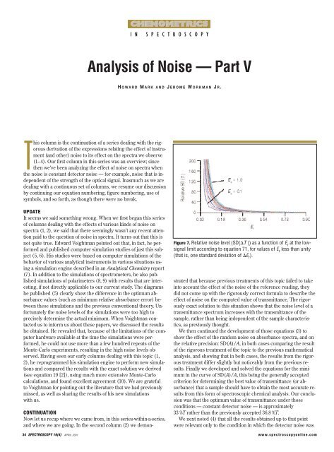
Figure 7. Relative noise level (SD(T )) as a function of E r at the lowsignal
limit according to equation 71, for values of E r less than unity
(that is, one standard deviation of E r ).
CONTINUATION
Now let us recap where we came from, in this series-within-a-series,
and where we are going. In the second column (2) we demonstrated
that because previous treatments of this topic failed to take
into account the effect of the noise of the reference reading, they
did not come up with the rigorously correct formula to describe the
effect of noise on the computed value of transmittance. The rigorously
exact solution to this situation shows that the noise level of a
transmittance spectrum increases with the transmittance of the
sample, rather than being independent of the sample characteristics,
as previously thought.
We then continued the development of those equations (3) to
show the effect of the random noise on absorbance spectra, and on
the relative precision: SD(A)/A, in both cases comparing the result
of the rigorous treatment of the topic to the previous mathematical
analysis, and showing that in both cases, the results from the rigorous
treatment differ slightly but noticeably from the previous results.
Finally we developed and solved the equations for the minimum
in the curve of SD(A)/A, this being the generally accepted
criterion for determining the best value of transmittance (or absorbance)
that a sample should have to obtain the most accurate results
from this form of spectroscopic chemical analysis. Our conclusion
was that the optimum value of transmittance under those
conditions — constant detector noise — is approximately
33 %T rather than the previously accepted 36.8 %T.
We next noted (4) that all the results obtained up to that point
were relevant only to the condition in which the detector noise was
34 SPECTROSCOPY 16(4) APRIL 2001 www.spectroscopyonline.com

...........................
CHEMOMETRICS IN SPECTROSCOPY ............................
small compared with the reference signal, and therefore the signalto-noise
ratio (S/N) was high. We then noted that if that condition
did not hold for any particular set of measurements, then other phenomena
also come into action. We pointed out that under low-noise
conditions the signal can affect the noise level, but under conditions
in which the signal is weak or the noise excessive, the noise can affect
the computed transmittance as well. The expressions we obtained
showed that as the reference signal gets weaker and weaker
(or the noise gets larger and larger), the system first reaches a
point at which the expected value of T is larger than E s
/E r
, and as
the reference signal continues to decrease, the multiplying factor
first goes through a maximum and then decreases so that the expected
value of T approaches zero as the reference signal energy,
E r
, approaches zero.
We are now ready to consider the behavior of the noise under
conditions in which it is not small compared with the signal.
We start with the definition of transmittance, as we pointed out
previously, and we rewrite the equation here:
T E s /E r [6]
To put equation 6 into a usable form under the conditions we
wish to consider, we could start from any of several points of view:
the statistical approach of Hald (11), for example, which starts from
fundamental probabilistic considerations and also derives confidence
intervals (albeit for various special cases only); the mathematical
approach (12) or the Propagation of Uncertainties approach
of Ingle and Crouch (13). Inasmuch as any of these starting points
will arrive at the same result when done properly, the choice of how
to attack an equation such as equation 6 is a matter of familiarity,
simplicity, and, to some extent, taste. We, being chemists and spectroscopists,
and writing for spectroscopists, will use the Propagation
of Uncertainties approach of Ingle and Crouch:
[64]
Note that we use the letters C,D to represent the variables in equation
64 to avoid confusion with our usage of A to mean absorbance.
Applying this to equation 6:
and apply first, the theorem that Var (A B) Var (A) Var (B):
and then the theorem that Var (aX) a 2 Var (X):
and continue as before by setting E s
E r
E:
and finally take square roots to obtain:
[68]
[69]
[70]
[71]
This is clearly a function of both E r and E s ; in the regime we are
concerned with in this column, however, as E r approaches zero, the
second term under the radical dominates the expression, although
clearly the point at which the numerical value becomes large compared
to 1/E r 2 will depend on the value of E s as well, or equivalently,
the transmittance of the sample. Here, again, therefore, the
behavior of the noise of the transmittance must be expressed as a
family of curves. Figures 7 and 8 present the behavior of this family
of curves as functions of E r and E s , respectively.
Note that equation 71 can be reduced to equation 19 (2), which is
appropriate when the signal-to-noise ratio is high and may be considered
constant. Under these conditions E r is large and the second
term under the radical is small and the first term under the radical,
which is independent of E s , dominates; then the noise of the trans-
As usual, we take the variance of this:
[65]
[66]
Figure 8. Relative noise
level (SD(T )) as a function
of E s at the lowsignal
limit according to
equation 71, for values of
E s between 0 and 1. The
lower plot (b) is an expansion
of the upper
plot (a).
[67]
APRIL 2001 16(4) SPECTROSCOPY 35

...........................
CHEMOMETRICS IN SPECTROSCOPY ............................
mittance increases with T as and inversely with the reference
energy.
Here, however, under low-signal, high-noise conditions, where
the variation of E r
cannot be ignored and therefore the signal-tonoise
ratio varies, we must use the full expression of equation 71.
Note further that when E r
is small enough, then, as mentioned earlier,
the second term under the radical dominates, then:
[72]
Table II. Value of integral of (1/E r
) 2 over the range 0.01 to
0.01.
Integration Interval
Value of Integral
10 2 2.0000000000000000e002
10 3 3.0995354623330845e003
10 4 3.2699678003698089e004
10 5 3.2878691333625099e005
10 6 3.2896681436917488e006
10 7 3.2898481337470137e007
The noise of the transmittance thus becomes directly proportional
to T and inversely proportional to E r
. Under these conditions
the noise of the transmittance approaches infinite values as E r
approaches
zero, even as the expected value of the transmittance approaches
zero, as we saw in the previous column(4).
To summarize the effects at low signal-to-noise to compare with
the high signal-to-noise case summarized earlier, here the noise of
the transmittance increases directly with T and still inversely with
the reference energy.
We now wish to follow through, as we did before, on finding the
optimum value for sample transmittance under these conditions. To
do this, we start with equation 24 (3):
[24]
This is the point at which, in the previous development, we considered
the effect of letting E r become negligible, but of course in
this case we wish to investigate the small-signal/large-noise behavior.
We now, therefore, go directly to dividing A by A (from equation
20b):
[73]
[74]
[75]
[76]
To determine the variance of A/A we perform our usual exercise
of taking the variance of both sides of equation 76 and applying
our two favorite theorems; the result is:
[77]
We cannot simplify this equation further; in particular, we cannot
separate out the variances of E s and E r to replace them with the
same generic value. To determine the variance of A/A — that is,
the relative precision (in chemist’s terms) — we need to evaluate
the variance of the two terms in equation 77. As we observed previously,
as the value of E r approaches E r , the value of the expressions
attains infinite values. However, a difference here is that when
the variance is computed these values are squared, and hence the
computations are always done using positive values. This differs
from our previous case, where the presence of both positive and
negative values afforded the opportunity for cancellation of near-infinite
contributions; we do not have that situation here. Therefore
we are faced with the possibility that the variance will be infinite.
An empirical test of this possibility was performed by computing
values of the variance of the two terms in equation 77. The normal
random number generator of MATLAB was used to create multiple
values of normally distributed random numbers for E r and E s ; these
were plugged into the two expressions of equation 77 and the variance
was computed. Between 10 2 and 10 6 values were used in each
computation of the variance.
When E r was more than five standard deviations away from the
center of the normal distribution representing E r , the computed
variance was fairly small and reasonably stable, and decreased as E r
was moved further away from the center of E r . This might be considered
an empirical determination of the point of demarcation of
the “small-signal” case.
When E r was moved below five standard deviations, the computed
value of the variance became very unstable; computed values
of the variance would differ by as much as four orders of magnitude.
The closer E r came to E r , the more erratic the computed
variance became. It was clear that bringing E r close to the center of
E r afforded more opportunity for a given reading of the noise to
become close to E r
, thus giving a value approaching infinity that
would be included in the calculation. Furthermore, for a given relationship
between E r
and E r
, the more readings that were included
in the computation, the higher the values of variance that would be
calculated. For example, with 100 readings, values of variance
might fall between 10 1 and 10 4 while, with 10,000 readings, calculated
variance values would fall in the range of approximately
36 SPECTROSCOPY 16(4) APRIL 2001 www.spectroscopyonline.com

...........................
CHEMOMETRICS IN SPECTROSCOPY ............................
10 3 –10 6 . This is attributed to the increased likelihood of more data
points being close to E r
and also of at least a few points being
closer to E r
than with fewer data.
Another test of whether the variance actually diverges and becomes
infinite is the same as the test we applied in the previous column:
to integrate the expressions in equation 77 in a small region
around the point E r
E r
using different intervals of integration
and see if the values converge or diverge. Basically, except for a
multiplying factor, these are both the same expression, so evaluating
the expression once suffices to settle the question for both of
them. Furthermore, because we are integrating over values of variance,
the expression that needs to be integrated is (1/E r
) 2 . The result
of performing this test is presented in Table II. In contrast to
the previous test results, the values are clearly growing increasingly
larger without bound as the integration interval is reduced.
The conclusion from all this is that the variance and therefore the
standard deviation attains infinite values when the reference energy
is so low that it includes the value zero. However, in a probabilistic
way, it is still possible to perform computations in this regime and
obtain at least some rough idea of how the various quantities involved
will change as the reference energy approaches zero. After
all, real data are obtained with a finite number of readings, each of
which is finite, and will give some finite answer. What we can do for
the rest of this current analysis is perform empirical computations
to find out what the expectation for that behavior is; we will do that
in the next column.
REFERENCES
(1) H. Mark and J. Workman, Spectroscopy 15(10), 24–25 (2000).
(2) H. Mark and J. Workman, Spectroscopy 15(11), 20–23 (2000).
(3) H. Mark and J. Workman, Spectroscopy 15(12), 14–17 (2000).
(4) H. Mark and J. Workman, Spectroscopy 16(2), 44–52 (2001).
(5) E. Voightman, Anal. Instrum. 21(1&2), 43–62 (1993).
(6) E. Voightman, Anal. Chem. 69(2), 226–234 (1997).
(7) E. Voightman, Anal. Chem. 65, 1029A–1035A (1993).
(8) E. Voightman, Anal. Chem. 64, 2590–2598 (1992).
(9) E. Voightman, Analyst 120, 325–330 (1995).
(10) E. Voightman, personal communication (2001).
(11) A. Hald, Statistical Theory with Engineering Applications (Wiley, New
York, 1952, pp. 115–118).
(12) G. A. Korn and T.M.Korn, Mathematical Handbook for Scientists and
Engineers (McGraw-Hill, New York, 1961, pp. 550–554).
(13) J.D. Ingle and S.R. Crouch, Spectrochemical Analysis (Prentice-Hall,
Upper Saddle River, NJ, 1988, p. 548).
Howard Mark and Jerome Workman Jr. serve on the Editorial Advisory
Board of Spectroscopy. Mark runs a consulting service, Mark Electronics,
21 Terrace Avenue, Suffern, NY 10901, that provides assistance,
training, and consultation in near-IR spectroscopy as well as
custom hardware and software design and development. He can be
reached via e-mail at hlmark@j51.com.Workman is a research fellow
at Kimberly-Clark Corporation, Neenah, WI 54956, (920) 721-
3988. He can be reached via e-mail at jworkman@kcc.com. ◆
Circle 25
APRIL 2001 16(4) SPECTROSCOPY 37