Mesh Clustering by Approximating Centroidal Voronoi Tessellation
Mesh Clustering by Approximating Centroidal Voronoi Tessellation
Mesh Clustering by Approximating Centroidal Voronoi Tessellation

You also want an ePaper? Increase the reach of your titles
YUMPU automatically turns print PDFs into web optimized ePapers that Google loves.
<strong>Mesh</strong> <strong>Clustering</strong> <strong>by</strong> <strong>Approximating</strong> <strong>Centroidal</strong> <strong>Voronoi</strong><br />
<strong>Tessellation</strong> ∗<br />
Fengtao Fan<br />
Depart. of Computer Science<br />
University of Kentucky<br />
ffan2@uky.edu<br />
Yong Li<br />
Depart. of Computer Science<br />
University of Kentucky<br />
yong.li@uky.edu<br />
Fuhua (Frank) Cheng<br />
Depart. of Computer Science<br />
University of Kentucky<br />
cheng@cs.uky.edu<br />
Jianzhong Wang<br />
Depart. of Computer Science<br />
University of Kentucky<br />
jwangf@uky.edu<br />
Conglin Huang<br />
Depart. of Computer Science<br />
University of Kentucky<br />
conglin.huang@uky.edu<br />
Shuhua Lai<br />
Depart. of Mathematics and<br />
Computer Science<br />
Virginia State University<br />
slai@vsu.edu<br />
ABSTRACT<br />
An elegant and efficient mesh clustering algorithm is presented.<br />
The faces of a polygonal mesh are divided into different<br />
clusters for mesh coarsening purpose <strong>by</strong> approximating<br />
the <strong>Centroidal</strong> <strong>Voronoi</strong> <strong>Tessellation</strong> of the mesh. The<br />
mesh coarsening process after clustering can be done in an<br />
isotropic or anisotropic fashion. The presented algorithm<br />
improves previous techniques in local geometric operations<br />
and parallel updates. The new algorithm is very simple but<br />
is guaranteed to converge, and comes out better approximating<br />
meshes with the same computation cost. Moreover,<br />
the new algorithm is suitable for the variational shape approximation<br />
problem with L 2,1 distortion error metric and<br />
the convergence is guaranteed. Examples demonstrating efficiency<br />
of the new algorithm are also included in the paper.<br />
Categories and Subject Descriptors<br />
I.3.5 [Computer Graphics]: Computational Geometry and<br />
Object Modeling —Physically based modeling<br />
Keywords<br />
<strong>Mesh</strong> <strong>Clustering</strong>, <strong>Centroidal</strong> <strong>Voronoi</strong> <strong>Tessellation</strong>, Shape Approximation<br />
1. INTRODUCTION<br />
3D mesh models are used in many important areas such as<br />
geometric modeling, computer animation, and CAD. With<br />
the availability of powerful laser scanners, large and dense<br />
meshes are easily acquired from physical world. However,<br />
∗ (Does NOT produce the permission block, copyright<br />
information nor page numbering). For use with<br />
ACM PROC ARTICLE-SP.CLS. Supported <strong>by</strong> ACM.<br />
since the full complexity of such models is not always required,<br />
coarsening a dense mesh, i.e., replacing the original<br />
mesh with a simpler but close enough mesh, is a necessary<br />
pre-processing step in many applications. Many mesh coarsening<br />
techniques have been presented, including the global<br />
optimization method [10, 18] and remeshing for mesh coarsening<br />
[22, 15, 13, 8].<br />
<strong>Mesh</strong> clustering is to partition the faces or vertices of the<br />
mesh into different regions. Generally, these regions are required<br />
to be nonoverlapping and connected. One major application<br />
of the clustering technique is for mesh coarsening.<br />
Such a method builds the approximating mesh based on the<br />
clustering of the dense mesh. In mesh coarsening, clustering<br />
may not be explicitly required in a greedy clustering technique,<br />
like mesh decimation. A decimation method creates<br />
implicit partitions of the mesh through greedy and repeatedly<br />
collapsing mesh faces or vertices [6, 9, 17]. The resulting<br />
mesh is always sub-optimal [2]. The other clustering method<br />
for mesh coarsening is to construct the mesh clusters explicitly.<br />
The new mesh clustering technique, also designed for<br />
mesh coarsening, falls into this category.<br />
There are quite a few papers discussing mesh approximation<br />
based on explicitly constructing clusters. <strong>Clustering</strong> <strong>by</strong><br />
approximating the <strong>Centroidal</strong> <strong>Voronoi</strong> <strong>Tessellation</strong> (CVT)<br />
[3] on triangular meshes is first discussed in [23]. After constructing<br />
the clusters, the mesh is uniformly coarsened based<br />
on the clusters. Adaptive coarsening of a mesh based on<br />
clustering from <strong>Centroidal</strong> <strong>Voronoi</strong> <strong>Tessellation</strong> is presented<br />
in [25]. An extension from uniform mesh coarsening [23] to<br />
anisotropic mesh coarsening is discussed in [24]. A theoretical<br />
framework of variational shape approximation based<br />
on optimal mesh clustering with respect to some distortion<br />
error metric is presented in [2]. Especially, optimal clustering<br />
using L 2,1 metric faithfully captures the anisotropic<br />
nature of the mesh. A hierarchical face clustering technique<br />
is developed in [19]. Many applications such as collision detection,<br />
surface simplification and multiresolution radiosity<br />
benefit from this hierarchical clustering technique. <strong>Clustering</strong><br />
faces in a set of characteristic regions to build a higherlevel<br />
description of mesh geometry is explored in [12, 21, 16,<br />
7]. Accelerating general iterative clustering algorithms for
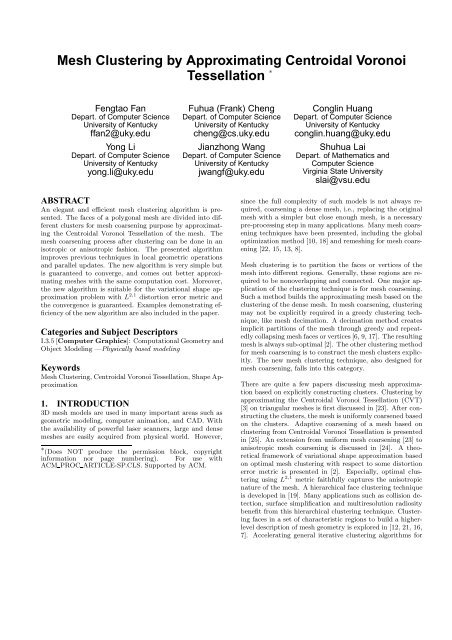
Figure 1: <strong>Clustering</strong> and approximation results on a hand model: the left-most figure shows the 500 clusters<br />
generated <strong>by</strong> approximating CVT on the mesh; the second from left figure is the uniformly coarsened mesh;<br />
the third from left figure has 98 clusters in different colors while using L 2,1 metric for clustering; the right-most<br />
figure is the approximating polygonal mesh.<br />
meshes on GPU is discussed in [11].<br />
This paper is inspired <strong>by</strong> the work presented in [23, 24, 2].<br />
The goal here is to do clustering <strong>by</strong> approximating constrained<br />
<strong>Centroidal</strong> <strong>Voronoi</strong> <strong>Tessellation</strong> [4] or <strong>Centroidal</strong><br />
<strong>Voronoi</strong> <strong>Tessellation</strong> [3] on a polygonal mesh. Starting with<br />
an initial partitioning of the mesh, the new algorithm iteratively<br />
tests the boundary edges between different clusters<br />
to update the cluster configuration until the boundary edges<br />
do not change any more. This boundary testing algorithm is<br />
also discussed in [23, 24]. But we derive a simpler algorithm<br />
<strong>by</strong> presenting a more rigorous mathematical analysis. The<br />
new algorithm is intuitive in that it only needs to compare<br />
the distances from one face centroid to centroids of adjacent<br />
clusters. The new algorithm is also extended for optimal geometric<br />
partitioning with respect to L 2,1 in [2]. The exciting<br />
result is that the new algorithm is guaranteed to converge<br />
while the algorithm based on Lloyd method in [2] is not. In<br />
summary, the contributions of this paper include:<br />
1. a simpler algorithm which only needs to compare distances<br />
is derived for constructing clusters on a polygonal<br />
mesh <strong>by</strong> approximating Constrained <strong>Centroidal</strong><br />
<strong>Voronoi</strong> Diagram or <strong>Centroidal</strong> <strong>Voronoi</strong> Diagram;<br />
2. the new algorithm updates cluster configurations after<br />
comparing all boundary edges, not after comparing<br />
each boundary edge. This updating scheme improves<br />
the quality of the output coarse mesh.<br />
3. the new algorithm for clustering with L 2,1 metric is<br />
guaranteed to converge. Sharing the same advantages<br />
of clustering with <strong>Centroidal</strong> <strong>Voronoi</strong> <strong>Tessellation</strong> methods,<br />
the new algorithm is fast.<br />
The remaining part of the paper is organized as follows: Section<br />
2 gives some basics on <strong>Centroidal</strong> <strong>Voronoi</strong> <strong>Tessellation</strong><br />
and its extension; Section 3 presents an analysis and the<br />
new clustering algorithm; Section 4 discusses the boundary<br />
testing algorithm for clustering with L 2,1 metric; Section 5<br />
proposes some strategies to make implementation more efficient;<br />
Section 6 gives applications of the new algorithm;<br />
test results are shown in Section 7; the conclusion is given<br />
in Section 8.<br />
2. CENTROIDAL VORONOI TESSELLATION<br />
<strong>Voronoi</strong> diagrams or <strong>Voronoi</strong> tessellation are essential structures<br />
in computational geometry and have been used in<br />
many important applications [20]. Given a domain Ω in<br />
R n and a set of points {z i} k i=1, the corresponding <strong>Voronoi</strong><br />
diagram {V i} k i=1 is a partition of Ω such that:<br />
(1) V i ∩ V j = ∅ and ∪ k i=1V i = Ω , and<br />
(2) V i = {x ∈ Ω | |x − z i| < |x − z j| for j = 1, 2, .., k, j ≠ i}<br />
{z i} k i=1 are called the generators and {V i} k i=1 the <strong>Voronoi</strong><br />
regions.<br />
<strong>Centroidal</strong> <strong>Voronoi</strong> <strong>Tessellation</strong> (CVT) is an extension of<br />
<strong>Voronoi</strong> <strong>Tessellation</strong> <strong>by</strong> requiring that the generators are<br />
also the mass centroids of the <strong>Voronoi</strong> regions. Given a<br />
density function ρ(x) on V , the mass centroid z ∗ of V is<br />
defined as<br />
R<br />
z ∗ V<br />
= R<br />
xρ(x)dx<br />
ρ(x)dx V<br />
Specifically, CVT of Ω is a minimizer of the energy functional<br />
[3] :<br />
nX<br />
Z<br />
F(z) = ρ(x)|x − z i| 2 dx (1)<br />
V i<br />
where z i ∈ Ω.<br />
i=1<br />
Constrained <strong>Centroidal</strong> <strong>Voronoi</strong> <strong>Tessellation</strong> [4] is the restriction<br />
of CVT to a surface. If a density function ρ(x) is<br />
defined on a surface S, we can define the constrained mass<br />
centroid z c of a region V ⊆ S as the solution to the following<br />
minimization problem:<br />
Z<br />
min<br />
z∈S<br />
V<br />
ρ(x)|x − z| 2 dx (2)<br />
A <strong>Voronoi</strong> <strong>Tessellation</strong> on a surface S is a Constrained <strong>Centroidal</strong><br />
<strong>Voronoi</strong> <strong>Tessellation</strong> (CCVT) if and only if the generators<br />
z i associated with each <strong>Voronoi</strong> region V i are also<br />
the constrained mass centroid of V i. Several applications of<br />
CCVT can be found in [4]. Furthermore, CCVT of surface<br />
S is also the minimizer of an energy functional similar to
the one defined in eq. (1) except now z i ∈ S [4]. Note<br />
that although x and z i are points of the surface S, CCVT<br />
uses the Euclidean distance instead of the geodesic distance.<br />
This minimization property is very important. We will take<br />
a deeper look of it in a later section. Several algorithms for<br />
constructing CVT and CCVT, such as the Lloyd method<br />
and k-means method, are presented in [3, 4].<br />
In this paper, we will show how to construct discrete CCVT<br />
and CVT on a polygonal mesh. Discrete CVT was thoroughly<br />
investigated in [23, 24]. Here, we will give a rigorous<br />
analysis of constructing CCVT on a polygonal mesh. We<br />
choose analyzing discrete CCVT because discrete CVT can<br />
be viewed as a special case of discrete CCVT. In fact, most<br />
of the examples presented in this paper are implemented<br />
to construct discrete CVT on triangular meshes. We first<br />
present our derivations below, then point out the differences<br />
from those in [23, 24].<br />
3. DISCRETE CONSTRAINED CENTROIDAL<br />
VORONOI TESSELLATION ON A POLYG-<br />
ONAL MESH<br />
Given a polygonal mesh M and a cluster number n, we<br />
will try to divide the faces of M into n connected sets of<br />
faces V i (i = 1,2, . . . , n) <strong>by</strong> constructing a CCVT on M.<br />
These clusters {V i} form a discrete CCVT on the mesh M.<br />
Although discrete CCVT can be defined for any polygonal<br />
mesh, we will concentrate on triangular meshes in this paper.<br />
In the continuous setting, CCVT is the minimizer of an energy<br />
functional similar to the one defined in eq. (1). For the<br />
discrete version of CCVT on a triangular mesh M, the region<br />
V i is a connected collection of triangles. We can rewrite<br />
the energy functional as<br />
nX<br />
„ X<br />
Z<br />
«<br />
F(z) =<br />
ρ(x)|x − z i| 2 dx<br />
i=1 T k ∈V T i k<br />
where T k ’s are triangles in V i. In this paper, we only consider<br />
the uniform case, i.e., ρ(x) = 1. Then the energy functional<br />
is<br />
F(z) =<br />
nX<br />
i=1<br />
„ X<br />
T k ∈V i<br />
Z<br />
In fact, the following equation holds<br />
Z<br />
|x − z i| 2 dx = |x k − z i| 2 |T k | + |T k|<br />
T k<br />
12<br />
«<br />
|x − z i| 2 dx<br />
T k<br />
(3)<br />
3X<br />
|x j k − x k| 2 (4)<br />
j=1<br />
where |T k | is the area of triangle T k with vertices x j k (j =<br />
1, 2,3) and x k is the centroid of T k . The derivation of this<br />
formula is shown in the appendix. Note that the second term<br />
on the right hand side is a constant for each triangle. We<br />
will use σ k to denote this term for triangle T k . Substituting<br />
the integral in eq. (3) with eq. (4), we have<br />
nX<br />
„ X<br />
«<br />
F(z) =<br />
|x k − z i| 2 |T k | + X<br />
σ k (5)<br />
i=1 T k ∈V i<br />
T k ∈M<br />
The last constant item is not essential in subsequent work,<br />
hence, will be omitted for F(z). The constrained mass centroid<br />
z i of V i on a continuous surface S is defined as a solution<br />
to the minimization problem defined in eq. (2) with<br />
V replaced with V i. For discrete CCVT on M, we can use<br />
the same argument as in reformulating F(z) to rewrite the<br />
minimization problem as:<br />
„ X<br />
min<br />
z∈M<br />
T k ∈V i<br />
|x k − z| 2 |T k | + X<br />
T k ∈V i<br />
σ k<br />
«<br />
The last constant item is not essential in the minimization<br />
process and, hence, will be omitted too. Furthermore, the<br />
above equation without the constant can be simplified as<br />
„ X<br />
«<br />
min<br />
z∈M<br />
where ¯z i =<br />
T k ∈V i<br />
|x k − ¯z i| 2 |T k | + X<br />
T k ∈V i<br />
|¯z i − z| 2 |T k |<br />
P<br />
T k ∈V i<br />
|T k |x k<br />
PT k ∈V i<br />
|T k |<br />
is the mass centroid of V i.<br />
A proof of eq. (6) can be found in the appendix. Thus the<br />
constrained mass centroid of V i is the point on M that is<br />
closest to its mass centroid ¯z i. Eqs. (5) and (6) are the<br />
counterparts of eqs. (1) and (2) in the discrete case. Before<br />
we describe the algorithm, two important properties have to<br />
be highlighted first.<br />
Property 3.1. Let {(V i,z i)} be the current cluster configuration<br />
where z i is the constrained mass centroid of V i,<br />
and for each triangle T r ∈ V i’s, let x r be its centroid. If<br />
|x k − z q| 2 < |x k − z p| 2 for some triangle T k ∈ V p and V q<br />
adjacent to V p, then<br />
where<br />
F ′ (z) =<br />
F ′ (z) < F(z)<br />
nX<br />
„ X<br />
i=1<br />
T k ∈V ′<br />
i<br />
z ′ i is the constrained mass center of V i ′ and<br />
8<br />
< V i i ≠ p, q<br />
V i ′ = V p − {T k } i = p<br />
:<br />
V q ∪ {T k } i = q .<br />
(6)<br />
«<br />
|x k − z ′ i| 2 |T k | , (7)<br />
Note that since |x k − z q| 2 < |x k − z p| 2 , it is clear that<br />
X<br />
X<br />
|x j − z p| 2 |T j| +<br />
|x j − z q| 2 |T j|<br />
T j ∈V p−{T k }<br />
< X<br />
T j ∈V q∪{T k }<br />
T j ∈V p<br />
|x j − z p| 2 |T j| + X<br />
T j ∈V q<br />
|x j − z q| 2 |T j|.<br />
From the minimization property of the constrained mass<br />
centroid z ′ i, the following inequality holds:<br />
X<br />
|x j − z ′ t| 2 |T j| ≤ X<br />
|x j − z t| 2 |T j| , t = p, q<br />
T j ∈V ′<br />
t<br />
T j ∈V ′<br />
t<br />
Combining these two steps, F ′ (z) < F(z) follows readily.<br />
Property 3.2. Let {(V i,z i)} be the current cluster configuration,<br />
and triangles T k ∈ V p and T s ∈ V q with centroids<br />
x k and x s, respectively, share a common edge. If
Figure 2: Illustration of 4 cases in distance comparison. The presence of an arrow indicates direction of the<br />
movement after the comparison. These are cases 1, 2, 3 and 4 from left to right in that order.<br />
|x k − z p| 2 > |x k − z q| 2 , |x s − z q| 2 > |x s − z p| 2 and |x k −<br />
z p| 2 |T k |+|x s −z p| 2 |T s| < |x k −z q| 2 |T k |+|x s −z q| 2 |T s| then<br />
F ′ (z) < F(z)<br />
where F ′ (z) is defined in eq. (7).<br />
This property can easily be proved following an argument<br />
similar to that of property 3.1. In fact, reassigning either T k<br />
or T s will lower the value of the energy functional F(z). In<br />
a greedy spirit, we simply choose the smaller one, which is<br />
reflected <strong>by</strong> the third given inequality. One can not simply<br />
assign T k to V q and T s to V p because the result could violate<br />
the connectivity requirement for clusters.<br />
3.1 Energy minimization<br />
Recall that a discrete CCVT of a triangular mesh M is a<br />
minimizer of the discrete energy functional (5). In the following<br />
we propose an algorithm to iteratively reduce the<br />
value of F(z) until a limit point is reached. The main idea<br />
of the algorithm is to update the clusters <strong>by</strong> comparing distances<br />
from triangle centroids of a cluster to mass centroids<br />
of adjacent clusters. The triangles that have to be considered<br />
are just boundary triangles, i.e., triangles sharing a cluster<br />
edge. A mesh edge is called a cluster edge if it is shared <strong>by</strong><br />
two triangle faces of different clusters. The distance comparing<br />
procedure is stated below.<br />
Let edge e lr be a cluster edge in the current cluster configuration<br />
{(V i,z i)}. e lr is shared <strong>by</strong> triangles T l and T r, where<br />
T l ∈ V p and T r ∈ V q are in different clusters. Let x l and x r<br />
be the centroids of T l and T r, respectively. Denote |x l −z p| 2 ,<br />
|x l −z q| 2 , |x r −z p| 2 and |x r −z q| 2 with d lp , d lq , d rp and d rq,<br />
respectively. We need to compare d lp with d lq , and d rp with<br />
d rq, totally four cases. Figure 2 illustrates these 4 cases.<br />
1. d lp ≤ d lq and d rp ≥ d rq.<br />
Do nothing. This is exactly what the convergent state<br />
should be.<br />
2. d lp ≤ d lq and d rp < d rq .<br />
Move T r to V p. According to property 3.1, this movement<br />
lowers the value of the energy functional F(z).<br />
3. d lp > d lq and d rp ≥ d rq .<br />
Move T l to V q. The new value of the energy functional<br />
F(z) will be lower, according to property 3.1.<br />
4. d lp > d lq and d rp < d rq .<br />
One more test is needed to decide which triangle should<br />
be moved.<br />
- If d lp |T l |+d rp|T r| < d lq |T l |+d rq|T r|, move T r to<br />
V p.<br />
- Otherwise, move T l to V q.<br />
The value of the energy functional F(z) will be lower<br />
after the movement, according to property 3.2.<br />
Based on this distance comparison process for a single it<br />
cluster edge, one can derive an algorithm which updates the<br />
mass centroids of the clusters immediately after finishing the<br />
above comparison process for each cluster edge. This algorithm<br />
should work because the energy functional decreases<br />
after the distance comparison process for each cluster edge.<br />
The problem with this algorithm is, it involves too many<br />
mass centroid updating steps for clusters. Instead, we propose<br />
an algorithm which would update the mass centroids<br />
of the clusters only after we finish distance comparison for<br />
all the cluster edges in the current cluster configuration. We<br />
call such a scheme configuration-wise updating. Correctness<br />
of such an approach is verified below.<br />
Let {(V i,z i)} be the current cluster configuration. Before<br />
the distance comparison process starts, two triangle sets V +<br />
i<br />
and V −<br />
i<br />
are attached to each cluster V i to record information<br />
during the distance comparison process. V +<br />
i records<br />
triangles not belonging to V i initially but are moved to V i<br />
somewhere during the comparison process. V −<br />
i<br />
records triangles<br />
belonging to V i initially but are moved to other clusters<br />
somewhere during the comparison process. Note that<br />
if T k ∈ V +<br />
i<br />
then there exists a j such that |x k − z i| 2 <<br />
|x k − z j| 2 . And if T k ∈ V −<br />
i then there exists a j such that<br />
|x k − z j| 2 < |x k − z i| 2 . It is clear that V +<br />
i<br />
∩ V −<br />
i<br />
= ∅. After<br />
the distance comparison process is done for all cluster edges,<br />
the new cluster V i ′ can be written as<br />
V ′<br />
i = (V i ∪ V +<br />
i ) − V −<br />
i<br />
We claim that the new energy functional is smaller, i.e.,<br />
F ′ (z) < F(z). This is shown below:<br />
nX<br />
„ X<br />
«<br />
F ′ (z) =<br />
|x k − z ′ i| 2 |T k |<br />
<<br />
=<br />
<<br />
i=1<br />
T k ∈V ′<br />
i<br />
nX<br />
„ X<br />
i=1<br />
nX<br />
„<br />
i=1<br />
nX<br />
„<br />
i=1<br />
= F(z)<br />
T k ∈V ′<br />
i<br />
X<br />
T k ∈V i −V −<br />
i<br />
X<br />
T k ∈V i −V −<br />
i<br />
«<br />
|x k − z i| 2 |T k |<br />
|x k − z i| 2 |T k | + X<br />
T k ∈V +<br />
i<br />
|x k − z i| 2 |T k | + X<br />
T k ∈V −<br />
i<br />
«<br />
|x k − z i| 2 |T k |<br />
«<br />
|x k − z i| 2 |T k |<br />
where z ′ i is the constrained mass centroid of V ′<br />
i and z i is the<br />
constrained mass centroid of V i. The first inequality follows
Figure 3: The left figure has 500 clusters. The right figure is a coarsened mesh <strong>by</strong> CVT.<br />
from optimality of the constrained mass centroid, and the<br />
second inequality follows from properties of V +<br />
i<br />
and V −<br />
i<br />
.<br />
Thus the new energy functional decreases after the one-time<br />
updating.<br />
The constrained mass centroid z i of the cluster V i is the<br />
closest point from M to the mass centroid ¯z i. ¯z i plays an<br />
important role in getting z i. In the following we derive a<br />
recursive formula to update the mass centroid ¯z i:<br />
¯z ′ i =<br />
where<br />
=<br />
=<br />
P<br />
T j ∈V<br />
i<br />
′ |T j |x j<br />
P<br />
T j ∈V<br />
i<br />
′ |T j |<br />
P<br />
T j ∈V |T i j |x j + P T j ∈V + |T j |x j − P T<br />
i<br />
j ∈V − |T j |x j<br />
P<br />
i<br />
T j ∈V<br />
i<br />
′ |T j |<br />
P<br />
T j ∈V |T i j | T<br />
P<br />
j ∈V + |T j |− P T<br />
i<br />
j ∈V − |T j |<br />
P<br />
i<br />
T j ∈V ′<br />
i<br />
var(¯z i ) =<br />
|T j |¯zi + P<br />
P<br />
T j ∈V +<br />
i<br />
P<br />
T j ∈V +<br />
i<br />
T j ∈V ′<br />
i<br />
|T j|x j − P T j ∈V −<br />
i<br />
|T j| − P T j ∈V −<br />
i<br />
|T j |<br />
var(¯z i )<br />
|T j|x j<br />
|T j|<br />
is the variation of the mass centroid z i. If the denominator<br />
equals zero, the new centroid will be computed directly.<br />
These are what we will record during the distance comparison<br />
process for cluster edges.<br />
The above comprehensive analysis induces an efficient clustering<br />
algorithm. With a valid initial cluster configuration,<br />
we perform distance comparison for each cluster edge<br />
and record the centroid variations of adjacent clusters at<br />
the same time. After completing the distance comparison<br />
process for all cluster edges, we update the mass centroids<br />
of clusters using eq. (8) and update the cluster edge set.<br />
This process is iterated until the cluster edge set no longer<br />
changes.<br />
It is obvious that the energy functional F(z) has a global<br />
minimum on the triangular mesh M. As F(z) decreases<br />
strictly after each configuration-wise updating, it is guaranteed<br />
to converge to a limit point. But the ”minimum” it<br />
achieves might not be the global minimum of F(z). For our<br />
clustering goal, it doesn’t matter much. The limit cluster<br />
configuration always gives a very good clustering of M.<br />
Remark: Although our results are for discrete CCVT on<br />
M, there are parallel results for discrete CVD on M ⊂ R 3 .<br />
(8)<br />
Because the mass centroid ¯z i =<br />
P<br />
T k ∈V i<br />
|T k |x k<br />
P<br />
T k ∈V i<br />
|T k |<br />
of a cluster V i<br />
on a triangular mesh M can also be viewed as a solution to<br />
the minimization problem<br />
This is true because we have<br />
X<br />
T k ∈V i<br />
|x k −z| 2 |T k | = X<br />
X<br />
min |x k − z| 2 |T k |<br />
z∈R 3 T k ∈V i<br />
T k ∈V i<br />
|x k −¯z i| 2 |T k |+ X<br />
T k ∈V i<br />
|¯z i −z| 2 |T k |<br />
Thus it is obvious that ¯z i is the solution to this minimization<br />
problem. We present the approximated results <strong>by</strong> CVT on<br />
the bunny model in Figure 3. The discrete CVT method<br />
runs much faster than the discrete CCVT method because<br />
the CCVT method needs to find the closest points in each<br />
iteration. Our examples in this paper are mainly the results<br />
from the discrete CVT method.<br />
Approximation of CVT on triangular meshes is also thoroughly<br />
discussed in [23, 24]. Especially, anisotropic approximation<br />
of CVT is also presented in [24]. The new algorithm<br />
is different from those in [23, 24] in two folds. First, the<br />
new algorithm has a simpler local geometric operation for<br />
cluster boundary test, namely, distance comparison. The<br />
methods in [23, 24] involve computation of certain terms<br />
of the energy functional, i.e. L iso,i = |z P i| 2 T k ∈V i<br />
|T k | −<br />
2z T i<br />
P<br />
T k ∈V i<br />
|T k |x k for each cluster V i in [24]. Their algorithm<br />
for L iso,i works as follows. For each cluster edge whose<br />
adjacent triangles are T i ∈ V p and T j ∈ V q, their algorithm<br />
computes L iso,p +L iso,q for 3 cases: 1) T i ∈ V p and T j ∈ V q;<br />
2) T i ∈ V p and T j ∈ V p; 3) T i ∈ V q and T j ∈ V q. The<br />
algorithm does the reassignment according to the minimum<br />
L iso,p + L iso,q of the 3 cases. The involved computation is<br />
less intuitive and lack of geometric meanings. Second, the<br />
new algorithm updates the cluster configuration after comparing<br />
all the cluster edges, while those algorithms in [23,<br />
24] update the clusters after comparing each cluster edge.<br />
The experimental differences will be discussed in Section 6<br />
(Applications). In addition to the above two differences, the<br />
new algorithm is also applicable to the variational shape approximation<br />
problem in [2], which will be discussed in the<br />
next section.<br />
4. BOUNDARY TESTING ALGORITHM FOR<br />
CLUSTERING WITH L 2,1 METRIC
A novel metric L 2,1 is introduced for geometric partitioning<br />
of a triangular mesh M in [2]. A geometric partition of M<br />
consists of a set of connected collections of triangles {R i} n i=1<br />
such that R i ∩ R j = ∅ (i ≠ j), ∪ n i=1R i = M and R i is<br />
connected. For each region R i, we can define a proxy plane<br />
P i = (X i,N i), where X i is the average point of the centroids<br />
and N i is the average normal of the triangles in R i. Given<br />
a region R i and its associated proxy plane P i, the L 2,1 for<br />
R i is defined as :<br />
Z Z<br />
L 2,1 (R i, P i) = |n(x) − N i| 2 dx<br />
x∈R i<br />
where n(x) is the normal of x ∈ R i. For triangular mesh, it<br />
can be precisely written as<br />
L 2,1 (R i, P i) = X<br />
T k ∈R i<br />
|n k − N i| 2 |T k |<br />
where n k is the unit normal of triangle T k and N i is the<br />
normalized vector of P T k ∈R i<br />
n k |T k |.<br />
Based on the L 2,1 metric, an optimal geometric partition of<br />
M and a given partition number n can be defined as the<br />
minimizer of the distortion error:<br />
nX<br />
E(M, P) = L 2,1 (R i, P i)<br />
i=1<br />
The advantage of using L 2,1 metric for shape approximation<br />
is thoroughly discussed in [2], i.e. anisotropy capturing. An<br />
algorithm for constructing an optimal geometric partition is<br />
also proposed in [2]. This algorithm always produces a good<br />
partition of M, but it is pointed out in [2] that it is not<br />
guaranteed to converge. Here, we develop a different algorithm<br />
for constructing an optimal geometric partition which<br />
minimizes the distortion error. This algorithm is based on<br />
boundary testing and distance comparison. It is very fast<br />
and convergent.<br />
Before proving convergence of the algorithm, we explore the<br />
minimization property of N i of the proxy plane first. Precisely,<br />
N i is the solution to the minimization problem:<br />
X<br />
min |n k − N| 2 |T k |<br />
|N|=1<br />
T k ∈R i<br />
Note that, similar to eq. (6), we have<br />
X<br />
T k ∈R i<br />
|n k −N| 2 |T k | = X<br />
T k ∈R i<br />
|n k −N i| 2 |T k |+ X<br />
where N i =<br />
P<br />
T k ∈R i<br />
n k |T k |<br />
PT k ∈R i<br />
|T k |<br />
. And it is obvious that<br />
|N i − N i| 2 = min |N − N i| 2<br />
|N|=1<br />
T k ∈R i<br />
|N i−N| 2 |T k |<br />
Thus the minimization property of N i follows. As far as<br />
a geometric partition is concerned, a region of a geometric<br />
partition is nothing but a cluster as we have discussed<br />
in the previous section. Thus boundary edges between different<br />
regions are just like cluster edges between different<br />
clusters. We will use the term cluster edge here too. Then<br />
for each cluster edge, there are also two properties similar to<br />
properties 3.1 and 3.2 for discrete CCVT.<br />
Property 4.1. Let {(R i,N i)} be the current geometric<br />
partition, and triangle T k ∈ R p with the unit normal n k . If<br />
|n k − N p| 2 > |n k − N q| 2 for some R q adjacent to R p, then<br />
E(M,R ′ ) < E(M, R)<br />
where E(M, R ′ ) = P „ «<br />
n P<br />
i=1 T k ∈R ′ |n k −N ′ i| 2 |T k |<br />
i<br />
the normalized vector of N i of R i ′ and<br />
8<br />
< R i i ≠ p,q<br />
R i ′ = R p − {T k } i = p<br />
:<br />
R q ∪ {T k } i = q<br />
, N ′ i is<br />
Property 4.2. Let {(R i,N i)} be the current cluster configuration,<br />
and triangles T k ∈ R p and T s ∈ R q, with unit<br />
normals n k and n s, respectively, share an edge e ks . If |n k −<br />
N p| 2 > |n k − N q| 2 , |n s − N q| 2 > |n s − N p| 2 and<br />
then<br />
|n k − N p| 2 |T k | + |n s − N p| 2 |T s|<br />
< |n k − N q| 2 |T k | + |n s − N q| 2 |T s|<br />
E(M,R ′ ) < E(M, R)<br />
where E(M,R ′ ) is the same as that in property 4.1.<br />
The correctness of properties 4.1 and 4.2 can be easily verified<br />
like properties 3.1 and 3.2 because of the optimality<br />
of N i. Besides, we can also update the unit normal N i of<br />
the proxy plane P i only after distance comparison for all<br />
cluster edges. The validity of such a configuration-wise updating<br />
is again based on the optimality of N i, same as the<br />
discrete CCVT. Another parallel result from discrete CCVT<br />
is that these N i can be computed recursively. N i of each<br />
proxy plane is of unit length. We can get it <strong>by</strong> normalizing<br />
the weighted normal N i for each region. We keep recording<br />
these N i for regions. Then we can update N i using a<br />
similar formula as eq. (8) <strong>by</strong> introducing the variation normal<br />
var(N i) for each region during the distance comparison<br />
process.<br />
Now we can deduce a convergent iterative algorithm for computing<br />
the optimal geometric partition with respect to the<br />
L 2,1 metric. This algorithm is similar to the boundary testing<br />
algorithm for CCVT. Starting with a valid initial geometric<br />
partition of M, we perform distance comparison for<br />
each cluster edge and record the variation normal var(N i)<br />
for each region at the same time. We then update the proxy<br />
unit normal N i <strong>by</strong> var(N i) and update the cluster edge<br />
sets. This process iterates until the cluster edge set doesn’t<br />
change any more.<br />
Note that this algorithm converges to a ”minimum” of the<br />
distortion error E(M, R). But it might not be the global<br />
minimizer of E(M, R). Nevertheless, test results show that<br />
this algorithm always converges to a near-optimal result<br />
quickly. For geometric partitioning, it would not be a problem<br />
to get a near-optimal partition. The theoretical advantage<br />
of the new algorithm is that it is guaranteed to convergent.<br />
We will discuss practical performance of this algorithm<br />
in the application section.
Figure 4: Illustration of edge contraction in dual graph (defined <strong>by</strong> solid edges) [19]. Left: dual graph before<br />
edge contraction; Right: dual graph after edge contraction, where two nodes in shaded area are merged into<br />
a single node.<br />
5. ACCELERATION STRATEGIES FOR IM-<br />
PLEMENTATION<br />
Several strategies can be used to accelerate the clustering<br />
process. We will explore several possibilities here, such as<br />
the ones considered in [24].<br />
5.1 Initialization<br />
Our iterative algorithm always begins with a valid initial<br />
cluster configuration, i.e., the clusters are connected and<br />
non-overlapping. A good initialization can reduce the clustering<br />
time significantly. We apply the hierarchical face clustering<br />
idea in [19] to design our cluster initialization. Hierarchical<br />
face clustering respects the connected requirement<br />
of clusters strictly. In the following we introduce a different<br />
edge contraction criterion for each distortion metric.<br />
The hierarchical face clustering is to partition the faces of<br />
a triangular mesh into different connected sets of faces. It<br />
builds such a hierarchical structure on the dual graph of the<br />
mesh. The dual graph is constructed <strong>by</strong> mapping each triangle<br />
in the mesh to a vertex in the dual graph, and generating<br />
an edge to connect two vertices if the corresponding triangles<br />
in the original mesh are adjacent. Then edge contraction is<br />
applied on the dual graph iteratively. An edge contraction<br />
merges two dual vertices into a single vertex. Figure 4 illustrates<br />
this concept. This means grouping two sets of faces<br />
into a single cluster. After each contraction, the dual graph<br />
is updated <strong>by</strong> replacing the two vertices with one vertex and<br />
associating edges adjacent to these two vertices to the new<br />
vertex. The edge chosen for contraction is based on a cost<br />
function. In [19], the cost function is the planarity criterion.<br />
For our algorithm, we define the cost function for an edge<br />
e ij that connects (V i,z i, |V i|) and (V j,z j, |V j|) as:<br />
F(e ij) = |zij − zi|2 |V i| + |z ij − z j| 2 |V j|<br />
|V i| + |V j|<br />
where |V p| = P T k ∈V p<br />
|T k | (p = i, j), z i and z j are the ”mass<br />
centroids” of V i and V j, respectively, and z ij = z i|V i |+z j |V j |<br />
|V i |+|V j |<br />
.<br />
z i depends on our distortion error metric. It is the mass centroid<br />
for the CVT constructing case and is the unit normal of<br />
the proxy plane for the optimal geometric partitioning case.<br />
The edge cost function F(e ij) is just the energy functional<br />
F(z) when there are only two faces V i and V j.<br />
Given the cluster number n, we first decide an number k such<br />
that the face number N f of the mesh satisfies n2 k < N f ≤<br />
n2 k+1 . Then we carry out k + 1 levels of edge contraction<br />
on the dual graph. For the initial level, we will contract<br />
N f − n2 k edges to reduce the nodes in dual graph to n2 k .<br />
For the next k levels of edge contraction, we will contract<br />
half of of edges in current dual graph to reduce half of the<br />
nodes. In the end, we will get exactly n clusters. It is always<br />
possible to sort the dual edges according to the value of its<br />
cost function. In order to speed the initialization process,<br />
we only sort the dual edges in the last few levels which have<br />
mush less edges. Our hierarchical initialization generates<br />
exactly n connected clusters and accelerates the clustering<br />
convergence.<br />
5.2 Accelerators<br />
Our algorithm converges. Thus only a few cluster edges need<br />
to be modified when the limit point is close. As pointed<br />
out in [24], one highly efficient strategy is to keep tracking<br />
whether a cluster is about to settle down. If it becomes<br />
static, then we don’t perform the distance comparison for<br />
cluster edges adjacent to this cluster any more. Another accelerating<br />
strategy is to trace potential cluster edges while<br />
doing distance comparison for current cluster edges. Precisely<br />
speaking, if a current cluster edge is not modified, it<br />
means the two triangles sharing this edge are not reassigned.<br />
Then we simply take itself as a potential edge. If it is modified,<br />
then we consider (the five) edges of the two adjacent<br />
triangles as potential edges. This potential edge tracking<br />
strategy also accelerates the clustering process.<br />
5.3 Validity of clusters<br />
As stated before, a valid cluster must be connected, but our<br />
algorithm does not guarantee that the resulting clusters are<br />
connected. In practice, a cluster might end up consisting<br />
of several distinct connected clusters. Once such a situation<br />
happens, we keep the largest non-isolated cluster and<br />
reassign triangles to other clusters that are closest to them.<br />
Another exception is that a cluster may be isolated, which<br />
means it is adjacent to a single cluster only. In such a situation,<br />
we just reassign the triangles to their closest clusters.<br />
In our experiments, these exceptions rarely happened when<br />
clustering <strong>by</strong> discrete CCVT or CVT. But they happened<br />
quite often when clustering <strong>by</strong> L 2,1 metric.<br />
6. APPLICATIONS<br />
Depending on the clustering criteria, a mesh M can either<br />
be uniformly coarsened after the construction of a discrete<br />
CVT or CCVT, or be approximated in an anisotropic fashion<br />
following the construction of an optimal geometric partition<br />
with respect to an L 2,1 metric. Uniform mesh coarsening<br />
and anisotropic approximation for L 2,1 metric are discussed<br />
in details in [23, 24] and [2], respectively. We will explore<br />
both techniques in our applications as well.<br />
6.1 Uniform <strong>Mesh</strong> Coarsening<br />
Once clustering of a mesh M <strong>by</strong> approximating CVT or<br />
CCVT is done, the following work of getting a coarsened
Figure 5: Results of uniform coarsening on a statue and a head model. The left most and the second from<br />
right figures are meshes with 800 clusters and 1000 clusters, respectively. The second from left and the right<br />
most figures are coarsened results.<br />
Models #F (org) #V (org) #V (approx) time(s) min∠ Ave. min ∠ ∠ < 30 ◦ Q min Q ave<br />
hand 72.9k 36.6k 1000 0.102 31.177 49.5895 0 0.580444 0.868164<br />
head 214k 107k 1000 2.11 34.3362 52.1764 0 0.597016 0.903267<br />
bunny 69.4k 34.8k 500 0.095 31.3123 50.321 0 0.581436 0.879907<br />
sphere 131k 65.5k 200 0.388 38.549 53.329 0 0.640395 0.915695<br />
horse 354k 177k 1.5k 6.24637 36.6344 51.6152 0 0.615523 0.897908<br />
statue 272k 136k 800 1.457 32.0611 51.9163 0 0.541623 0.900297<br />
Table 1: Results for uniform mesh coarsening<br />
triangular mesh is relatively simple. The process is like a<br />
Delaunay triangulation, with each cluster treated as a logical<br />
vertex. The process is illustrated below.<br />
First, a vertex is created for each cluster. Several techniques<br />
can be used here. One approach is, for each cluster, take<br />
the vertex that is closest to its mass centroid [23]. A second<br />
choice is to use the Quadric Error Metric to compute a vertex<br />
[24]. The first approach is used here since it conforms more<br />
with the spirit of CCVT on a mesh.<br />
The second step is to triangulate the vertices created in the<br />
above step. Delaunay triangulation is used here. Two vertices<br />
are connected with an edge in the coarsened mesh if the<br />
corresponding clusters of these vertices are adjacent to each<br />
other. Thus a vertex point that is shared <strong>by</strong> three clusters<br />
corresponds to a triangle in the coarsened mesh. Degenerate<br />
cases, however, would arise if a vertex point is shared <strong>by</strong><br />
more than 3 clusters. The solution to such degenerate cases<br />
is quite simple. If a vertex point is shared <strong>by</strong> n (≥ 4) clusters,<br />
then there would be an n-side polygon in the coarsened<br />
mesh corresponding to this vertex point. We simply triangulate<br />
this polygon to get n −2 triangles. Hence the output<br />
coarsened mesh is always a triangular mesh. Examples are<br />
shown in the next section.<br />
6.2 Anisotropic Shape Approximation<br />
After getting an optimal geometric partition with respect to<br />
the L 2,1 error metric, one can use the strategy presented in<br />
[2] to construct an anisotropic polygonal mesh to approximate<br />
the original mesh.<br />
The first step is anchor vertex creation. An anchor vertex<br />
corresponds to a vertex in the original mesh that is shared<br />
<strong>by</strong> more than 3 clusters. The position of the anchor vertex<br />
is the average of the projections of the corresponding vertex<br />
to its shared clusters. The next step is edge extraction.<br />
A vertex corresponding to an anchor vertex is connected to<br />
other such vertices <strong>by</strong> cluster edges in the original mesh. We<br />
connect two anchor vertices if their corresponding vertices<br />
are linked with cluster edges and there are no other such<br />
vertices between them. Because of anisotropic property, an<br />
edge between two anchor vertices may not faithfully capture<br />
the geometry on the original mesh. Therefore, sometime it is<br />
necessary to insert new anchor vertices between two anchor<br />
vertices to get more edges according to some criteria such<br />
as: d · sin(N i,N j)/ ‖(a,b)‖ is less than a threshold, where<br />
‖(a,b)‖ is the distance between a and b, d is the largest distance<br />
from the vertices on the boundary arc in the original<br />
mesh to (a,b) and (N i,N j) is the angle between the two<br />
adjacent clusters R i and R j. After edge contraction, triangulation<br />
is performed. A multi-source Dijkstra’s shortest<br />
path algorithm is applied to do the pseudo-Constrained Delaunay<br />
Triangulation, which will preserve the edges on the<br />
boundary in the final triangulation. In this algorithm, each<br />
anchor vertex represents a color. This algorithm first colors<br />
vertices in the original mesh which are on the boundary<br />
with the color of the closest anchor vertex. Then do color<br />
assignment for interior points in each cluster. Then for each<br />
triangle in the original mesh whose three vertices have distinct<br />
colors, we create a triangle in the approximating mesh<br />
whose edges are connected according to the colors in the<br />
referring triangle. More on postprocessing is discussed in<br />
detail in [2]. To clearly show the anisotropic effect, we only<br />
show polygonal mesh representations of the examples used<br />
in this paper.<br />
7. RESULTS
Models #F (org) #V (org) #F (approx) time(s)<br />
hand 72.9k 36.6k 98 1.542<br />
face 98.4k 49.3k 119 1.084<br />
fandisk 12.9k 6.4k 32 0.032<br />
monster 130k 65k 120 1.8327<br />
Table 2: Results for anisotropic mesh approximation<br />
The algorithms presented in this paper are implemented on<br />
a laptop computer with 1G memory and Intel Core 2 CPU<br />
T7200 under Windows. Performance data for uniform mesh<br />
coarsening applications are collected in Table 1. Experimental<br />
data for anisotropic shape approximation are gathered in<br />
Table 2. Notice that the new algorithms run very fast. It<br />
takes only a few seconds to get the job done for a mesh with<br />
more than 200k faces.<br />
For the uniform mesh coarsening application, the quality of<br />
the output mesh M is measured in several aspects, as listed<br />
in Table 1. ’min ∠’ stands for the minimum angle degree of<br />
the triangle faces in M. Similarly, ’Ave. min ∠’ computes<br />
the average minimum angle degree. ’∠ < 30 ◦ ’ counts the<br />
number of angles smaller than 30 degrees. ’Q min’ (minimal<br />
quality) and ’Q ave’ (average quality) measure the triangle<br />
shapes. Both terms are defined in [5]. The examples have<br />
also been tested using the program provided <strong>by</strong> the authors<br />
of [23, 24]. The execution times for models bunny and hand<br />
are 0.328s and 0.266s, respectively, which are slower than<br />
the new algorithm. However, the execution times on the<br />
statue model and the horse model are 0.954s and 1.547s,<br />
respectively, which are better than the new algorithm. But<br />
the output meshes of the new algorithms always have better<br />
mesh quality. For instance, for the sphere model, the data<br />
generated <strong>by</strong> the program of [23, 24] are min ∠ = 37.7732,<br />
Ave. min ∠ = 52.8697, ∠ < 30 ◦ = 0, Q min = 0.710607 and<br />
Q ave = 0.9096. Data generated <strong>by</strong> the new algorithm are<br />
better.<br />
From Table 2, one can see that the new algorithm runs very<br />
fast and gives good approximation results. This shows that<br />
the new algorithm is practical. The new algorithm contracts<br />
one face for each cluster. Then the number of clusters in the<br />
clustering result for each mesh is just the ’#F (approx)’ in<br />
Table 2, such as 32 clusters for the fandisk model. The<br />
anisotropic nature of the L 2,1 error metric is demonstrated<br />
in these examples.<br />
8. CONCLUSIONS<br />
In this paper we propose a novel clustering algorithm for<br />
a polygonal mesh M <strong>by</strong> approximating CVT or CCVT on<br />
M. The new clustering algorithm is also suitable for clustering<br />
construction with respect to the L 2,1 error metric.<br />
We present a rigorous mathematical analysis for the new<br />
algorithm. Our algorithm possesses the intrinsic distance<br />
comparison as the local geometric operation, which is simpler<br />
and more intuitive than those used in [23, 24]. Moreover,<br />
our algorithm updates the cluster configuration only<br />
after comparing all cluster edges. The proposed algorithm<br />
based on Lloyd method for constructing the optimal geometric<br />
partition in [2] is not guaranteed to converge. But<br />
the new algorithm is proved to converge for constructing discrete<br />
CCVT and CVT on M or clustering with L 2,1 metric.<br />
Although the new algorithm runs more or less as those in<br />
[24], the coarse mesh produced <strong>by</strong> the new algorithm has a<br />
better mesh quality. Depending on the clustering criteria,<br />
we show examples for both isotropic and anisotropic mesh<br />
approximations. The anisotropic mesh approximation <strong>by</strong> using<br />
CVT is also investigated in [24]. It seems an interesting<br />
problem to generalize the new algorithm for the anisotropic<br />
case. This will be investigated in the future.<br />
APPENDIX<br />
A. INTEGRATION OVER A TRIANGLE<br />
Suppose the triangle T k has three vertices x 1, x 2, x 3. Let<br />
x ∈ T k . Then we have x = λ 1(x)x 1 + λ 2(x)x 2 + λ 3(x)x 3,<br />
where λ i(x)(i = 1, 2,3) are the barycentric coordinates of x.<br />
We have P 3<br />
i=1<br />
λi(x) = 1. Then<br />
Z<br />
T k<br />
|x − z i| 2 dx =<br />
=<br />
=<br />
Z<br />
|λ 1(x)x 1 + λ 2(x)x 2 + λ 3(x)x 3 − z i| 2 dx<br />
T k<br />
Z 3X<br />
λ j(x)(x j − z i)| 2 dx<br />
T k<br />
|<br />
3X<br />
Z<br />
j=1<br />
λ j(x) 2 |x j − z i| 2 dx<br />
j=1 T k<br />
Z<br />
+2 λ 1(x)λ 2(x) < x 1 − z i,x 2 − z i > dx<br />
T<br />
Z k<br />
+2 λ 1(x)λ 3(x) < x 1 − z i,x 3 − z i > dx<br />
T<br />
Z k<br />
+2 λ 2(x)λ 3(x) < x 2 − z i,x 3 − z i > dx<br />
T k<br />
Using the fact that R T k<br />
λ i(x)λ j(x)dx = |T k |/12 (i ≠ j) and<br />
R<br />
T k<br />
λ i(x) 2 dx = |T k |/6 (i = 1, 2, 3) (see [1]), we have<br />
Z<br />
|x−z i| 2 dx = |T k|<br />
T k<br />
6<br />
` 3X<br />
|x j−z i| 2 + X<br />
j=1<br />
1≤r ´
This equality is also a special case of [14]. Consequently, we<br />
have<br />
Z<br />
|x − z i| 2 dx = |T k| ` 3X<br />
|x j − x k + x k − z 2´<br />
i|<br />
T k<br />
12<br />
where x k =<br />
P 3i=1<br />
x i<br />
3<br />
.<br />
+ |T k|<br />
12<br />
j=1<br />
+ X<br />
= |T k|<br />
12<br />
` 3X<br />
|x j − z i| 2<br />
j=1<br />
1≤r ´<br />
` 3X<br />
|x j − x k | 2 + 3|x k − z 2´<br />
i|<br />
j=1<br />
+ 9|T k|<br />
12 |x k − z i| 2<br />
= |T k|<br />
12<br />
` 3X<br />
|x j − x k | 2´ + |x k − z i| 2 |T k |<br />
j=1<br />
B. EXPANSION WITH THE MASS CENTROID<br />
Let ¯z i =<br />
P<br />
T k ∈V |T i k |x k<br />
PT k ∈V i<br />
|T k |<br />
be the mass centroid of V i. ¯z i satisfies<br />
the following equation<br />
X<br />
Consequently,<br />
X<br />
T k ∈V i<br />
|x k − z| 2 |T k | = X<br />
T k ∈V i<br />
|T k |(x k −¯z i) = 0<br />
T k ∈V i<br />
|x k −¯z i + ¯z i − z| 2 |T k |<br />
= X<br />
T k ∈V i<br />
`|xk −¯z i| 2 + 2 < x k −¯z i,¯z i − z ><br />
+|¯z i − z| 2´|T k |<br />
= 2 < X<br />
|T k |(x k −¯z i),¯z i − z ><br />
T k ∈V i<br />
+ X<br />
|x k − ¯z i| 2 |T k | + X<br />
|¯z i − z| 2 |T k |<br />
T k ∈V i T k ∈V i<br />
= X<br />
|x k −¯z i| 2 |T k | + X<br />
|¯z i − z| 2 |T k |<br />
T k ∈V i T k ∈V i<br />
Figure 7: <strong>Clustering</strong> and coarsening results for a<br />
horse model. Top: a mesh with 1500 clusters. Bottom:<br />
coarsened mesh.<br />
Figure 6: <strong>Clustering</strong> and coarsening results for a<br />
sphere model. Left: a sphere with 200 clusters.<br />
Right: coarsened mesh.<br />
C. REFERENCES<br />
[1] L. Chen. New analysis of the sphere covering problems<br />
and optimal polytope approximation of convex bodies.<br />
J. Approx. Theory, 133(1):134–145, 2005.<br />
Figure 8: Two different views of clustering and approximation<br />
of a monster model with 120 clusters.
Figure 9: Two different views of clustering and approximation<br />
of a face model with 119 clusters<br />
Figure 10: Two different views of clustering and approximation<br />
of a fandisk model with 32 clusters<br />
[2] D. Cohen-Steiner, P. Alliez, and M. Desbrun.<br />
Variational shape approximation. ACM Transactions<br />
on Graphics. Special issue for SIGGRAPH conference,<br />
pages 905–914, 2004.<br />
[3] Q. Du, V. Faber, and M. Gunzburger. <strong>Centroidal</strong><br />
voronoi tessellations: Applications and algorithms.<br />
SIAM Rev., 41(4):637–676, 1999.<br />
[4] Q. Du, M. D. Gunzburger, and L. Ju. Constrained<br />
centroidal voronoi tessellations for surfaces. SIAM J.<br />
Sci. Comput., 24(5):1488–1506, 2002.<br />
[5] P. Frey and H. Borouchaki. Surface mesh evaluation.<br />
In 16th International <strong>Mesh</strong>ing Roundtable, pages<br />
363–374, 1997.<br />
[6] M. Garland and P. S. Heckbert. Simplifying surfaces<br />
with color and texture using quadric error metrics. In<br />
VIS ’98: Proceedings of the conference on<br />
Visualization ’98, pages 263–269, Los Alamitos, CA,<br />
USA, 1998. IEEE Computer Society Press.<br />
[7] E. Grinspun and P. Schröder. Normal bounds for<br />
subdivision-surface interference detection. In VIS ’01:<br />
Proceedings of the conference on Visualization ’01,<br />
pages 333–340, Washington, DC, USA, 2001. IEEE<br />
Computer Society.<br />
[8] I. Guskov, K. Vidimče, W. Sweldens, and P. Schröder.<br />
Normal meshes. In SIGGRAPH ’00: Proceedings of<br />
the 27th annual conference on Computer graphics and<br />
interactive techniques, pages 95–102, New York, NY,<br />
USA, 2000. ACM Press/Addison-Wesley Publishing<br />
Co.<br />
[9] H. Hoppe. Progressive meshes. In SIGGRAPH ’96:<br />
Proceedings of the 23rd annual conference on<br />
Computer graphics and interactive techniques, pages<br />
99–108, New York, NY, USA, 1996. ACM.<br />
[10] H. HOPPE, T. DEROSE, T. DUCHAMP,<br />
J. MCDONALD, and W. STUETZLE. <strong>Mesh</strong><br />
optimization. In ACM SIGGRAPH Proceedings, pages<br />
19–26, 1993.<br />
[11] J. C. H. Jesse D. Hall. Gpu acceleration of iterative<br />
clustering. The ACM Workshop on General Purpose<br />
Computing on Graphics Processors, and SIGGRAPH<br />
2004 poster, Aug. 2004.<br />
[12] A. Kalvin and R. Taylor. Superfaces: Polygonal mesh<br />
simplification with bounded error. IEEE Comput.<br />
Graph. Appl., 16(3):64–77, 1996.<br />
[13] L. Kobbelt, J. Vorsatz, U. Labsik, and H.-P. Seidel. A<br />
shrink wrapping approach to remeshing polygonal<br />
surfaces. 18(3):119–130, 1999. (Proceedings of<br />
EUROGRAPHICS’99).<br />
[14] J. B. Lasserre and K. E. Avrachenkov. The<br />
multi-dimensional version of R b<br />
a xp dx. The American<br />
Mathematical Monthly, 108(2):151–154, 2001.<br />
[15] A. W. F. Lee, W. Sweldens, P. Schröder, L. Cowsar,<br />
and D. Dobkin. Maps: multiresolution adaptive<br />
parameterization of surfaces. In SIGGRAPH ’98:<br />
Proceedings of the 25th annual conference on<br />
Computer graphics and interactive techniques, pages<br />
95–104, New York, NY, USA, 1998. ACM.<br />
[16] B. Lévy, S. Petitjean, N. Ray, and J. Maillot. Least<br />
squares conformal maps for automatic texture atlas<br />
generation. ACM Trans. Graph., 21(3):362–371, 2002.<br />
[17] P. Lindstrom and G. Turk. Fast and memory efficient
polygonal simplification. In VIS ’98: Proceedings of<br />
the conference on Visualization ’98, pages 279–286,<br />
Los Alamitos, CA, USA, 1998. IEEE Computer<br />
Society Press.<br />
[18] P. Lindstrom and G. Turk. Image-driven<br />
simplification. ACM Trans. Graph., 19(3):204–241,<br />
2000.<br />
[19] A. W. M. Garland and P. S. Heckberty. Hierarchical<br />
face clustering on polygonal surfaces. In Proceedings of<br />
the Symposium on Interactive 3D Graphics, 2001.<br />
[20] A. Okabe, B. Boots, and K. Sugihara. Spatial<br />
<strong>Tessellation</strong>s Concepts and Applications of <strong>Voronoi</strong><br />
Diagrams. John Wiley & Son, 1992.<br />
[21] A. Sheffer. Model simplification for meshing using face<br />
clustering. Comptuer-Aided Design, 33:925–934, 2001.<br />
[22] G. Turk. Re-tiling polygonal surfaces. SIGGRAPH<br />
Comput. Graph., 26(2):55–64, 1992.<br />
[23] S. Valette and J.-M. Chassery. Approximated<br />
centroidal voronoi diagrams for uniform polygonal<br />
mesh coarsening. 23(3):381–389, 2004. (Proc.<br />
Eurographics’04).<br />
[24] S. Valette, J.-M. Chassery, and R. Prost. Generic<br />
remeshing of 3d triangular meshes with<br />
metric-dependent discrete voronoi diagrams. IEEE<br />
Transactions on Visualization and Computer<br />
Graphics, 10(2):369–381, 2008.<br />
[25] S. Valette, I. Kompatsiaris, and J.-M. Chassery.<br />
Adaptive polygonal mesh simplification with discrete<br />
centroidal voronoi diagrams. In Proceedings of 2nd<br />
International Conference on Machine Intelligence<br />
ICMI 2005, pages 655–662, 2005.