1 - Computer Science Department - University of Kentucky

CS537
Introduction to Numerical
Methods
Lecture 2
Interpolation and Numerical
Differentiation
Professor Jun Zhang
Department of Computer Science
University of Kentucky
Lexington, KY 40206‐0046
September 12, 2013

Polynomial Interpolation
Given a set of discrete values, how can we estimate other values
between these data
The method that we will use is called polynomial interpolation.
We assume the data we had are from the evaluation of a smooth
function. We may be able to use a polynomial p(x) to approximate this
function, at least locally.
A condition: the polynomial p(x) takes the given values at the given
points (nodes), i.e., p(x i ) = y i with 0 ≤ i ≤ n. The polynomial is said to
interpolate the table, since we do not know the function.
2

Polynomial Interpolation
Note that all the points are passed through by the curve
3

Polynomial Interpolation
We do not know the original function, the interpolation
may not be accurate outside the set of data points
4

Order of Interpolating Polynomial
A polynomial of degree 0, a constant function, interpolates one set of data
If we have two sets of data, we can have an interpolating polynomial of
degree 1, a linear function
x x1
x x0
p(
x)
y0
y1
x0
x1
x1
x0
Review carefully if the condition is satisfied
y
0
y
x
Interpolating polynomials can be written in several forms, the most well
known ones are the Lagrange form and Newton form. Each has some
advantages
1
1
y
x
0
0
(
x x
0
)
5

Lagrange Form
For a set of fixed nodes x 0 , x 1 ,…,x n , the cardinal functions, l 0 , l 1 ,…, l n ,
are defined as
0
if i j
li
( x j ) ij
1
if i j
We can interpolate any function f(x) by the Lagrange form of the
interpolating polynomial of degree ≤ n
p
Note that l i (x) is of order n, so p n (x) is of order ≤ n, and
p
n
( x
j
)
n
i1
l
i
The (point exact) interpolation condition is satisfied
n
( x
( x)
j
) f ( x
n
i0
i
)
l
i
( x)
f ( x
l
j
( x
j
i
)
) f ( x
j
)
f ( x
j
)
6

Cardinal Functions
7
The cardinal function is
What it looks like
Note that
and
n
j
i
j
j
i
j
i
n
i
x
x
x
x
x
l
0
,
)
(0
)
(
n
i
n
i
i
i
i
i
i
i
i
i
x
x
x
x
x
x
x
x
x
x
x
x
x
x
x
x
x
x
x
x
x
l
1
1
1
1
1
1
0
0
)
(
j
i
x
l
j
i
for
0,
)
(
1
)
(
l i x i

Five Lagrange Basis Polynomials
These are the 5 Lagrange basis polynomials for N=5
8

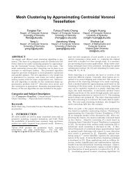
Representation by Lagrange Polynomials
Five weighted polynomials and their sum (red line) for a
set of 5 random samples (red points)
9

Step by Step Construction
For any table of data, we can construct a Lagrange interpolating
polynomial. Its evaluation is a little bit costly, but we can always do that.
The existence of the interpolating polynomial is guaranteed
Can we construct the interpolating polynomial step by step, or if we
discover some new data, can we add those data to the existing
interpolating polynomial to make the interpolation more accurate?
We can use Newton form of the interpolating polynomial
Let p k (x) be an interpolating polynomial for the date set {(x i ,y i )} with
0 ≤ i ≤ k such that p k (x i ) = y i
10

Newton Form ‐ Cont.
We want to add another data (x k+1 , y k+1 ) to have a new interpolating
polynomial p k+1 (x) such that p k+1 (x i ) = y i for 0 ≤ i ≤ (k + 1).
Let
p x)
p ( x)
c(
x x )( x x ) (
x x )
where c is an undetermined constant
Since
p
k1( k
0 1
k
( x k 1)
y 1,
p ( x
k 1 k
k
k1
(
x
we have
) c(
x
k1
x
k
k1
)
We can solve this equation for c, with the condition that x 0 , x 1 , …, x k+1 are
all distinct
yk
1
pk
( xk1)
c
( x x )( x x ) (
x x )
k 1
0
k1
y
x
0
k1
1
)( x
k1
k1
x
1
)
k
11

Newton Polynomial Interpolation
12

Uniqueness of Polynomial
Is the interpolating polynomial unique?
If p and q are interpolating polynomials for the data set {(x i ,y i )} for 0 ≤ i ≤ n
such that p(x i ) = q(x i ) = y i
Then the polynomial r(x) = p(x) – q(x) of degree at most n is zero at x 0 , x 1 ,
…, x n . Note that a polynomial of degree n can have at most n roots, we
must have r(x) = 0, or p – q = 0. Hence p = q
The interpolating polynomial is unique
It may be written in different forms
13

An Example
Find the interpolating polynomial for this table
Lagrange form
l
l
0
1
( x)
( x)
( x 1)( x 1)
(0 1)(0 1)
( x 0)( x 1)
(1 0)(1 1)
( x 0)( x 1)
l2(
x)
( 1
0)( 1
1)
The interpolating polynomial is
(
x 1)( x 1)
1
2
x(
x 1)
1
2
x(
x 1)
3 15
p2(
x)
5( x 1)( x 1) x(
x 1) x(
x 1)
2 2
14

Newton Form
The zeroth order polynomial is
p0(
x)
5
Let the 1 st order interpolating polynomial be
p
( x)
p0
c(
x x0
)
We want p 1 (x 1 ) = -3, hence -5 + c(1 – 0) = -3, we have c = 2, it follows that
Let the 2 nd order interpolating polynomial be
5
c(
x
1
p
p ( x)
5
2x
1
( x)
p1(
x)
c(
x x0
)( x 1)
2 x
Put p 2 (-1) = -15, i.e., -5+2(-1) + c(-1 – 0)(-1 – 1) = -15. We have c = -4.
The Newton form of the interpolating polynomial is
p2(
x)
5
2x
4x(
x 1)
0)
15

Nested Form
For easy programming and efficient computation, we can write Newton
form of the interpolating polynomial in nested form
p(
x)
a
a
a
0
3
a1[(
x x0
)] a2[(
x x0
)( x
[( x x0
)( x x1)(
x x2
)]
[( x x )( x x ) (
x )]
n 0 1 x n 1
x
1
)]
Or, using standard product notations as
n i1
p(
x)
a ai (
x x j
i1
j1
Using successive factorization, the nested form is
p(
x)
a ( x x )( a ( x x )( a
0
( x x
( ((
a
a
n
n2
0 )
0
n1
) a
( x x
1
n
n1
) )(
x x
)) )
) a
0
n1
) a
0
1
2
)( x x
n2
)
16

Computation Procedure
To evaluate p(x) for a given x, we start from the innermost parentheses, forming
successively some intermediate quantities
v
v
v
v
v
0
1
2
i
n
a
v
v
v
v
n
0
1
( x x
( x x
i1
n1
n1
n2
( x x
( x x
ni
0
) a
) a
) a
n1
n2
) a
0
ni
A pseudocode is
real array ( ai
) 0: n , ( xi
) 0:
integer i,
n
real x,
v
v an
for i n 1 to 0 step -1do
v
v(
x
xi
) ai
end for
n
17

Divided Difference
The coefficients a i in Newton form of the interpolating polynomial need to
be computed. A notation is introduced to facilitate such computation
a
which is called the divided difference of order k for f
k
f[ x , x1,
,
x
0 k
]
Newton form interpolating polynomial is
p ( x)
a
Or written in a compact form
with the convention
n
0
a
a
p
1
( x x
n
n
0
( x x
( x)
1
j0
n
0
) a
2
( x x
) (
x x
ai
i0
( x
i1
j0
x j
( x x
) 1
j
0
n1
)
)( x
)
x
1
)
18

Computing Coefficients a i
We want p n (x i ) = f(x i ). So we have
f
f
f
( x
( x
( x
) a
) a
) a
The solution of this system is
0
1
2
0
0
0
a
a
1
1
( x
1
( x
2
x
0
x
a
0
)
) a
0 x
2
(
f ( 0 )
x
2
x
0
)(
x
2
x
1
)
a
1
f ( x1)
a0
x1
x0
f ( x1)
f ( x
x x
The divided difference of order 1 is
f ( x1)
f ( x0
)
f [ x0
, x1]
x1
x0
Note that f[x 0 , x 1 ,…, x k ] is the coefficient of x k in the polynomial p k of
degree ≤ k
1
0
0
)
19

Computing Coefficients –Cont.
f ( x2
) a0
a1(
x2
x0
)
a2
( x2
x0
)( x2
x1)
f ( x2
) f [ x0
] f [ x0
, x1](
x2
x
( x2
x0
)( x2
x1)
f [ x0
, x1,
x2
]
In general, we have
f [ x0
, x1,
,
xk
]
k1
f ( x ) f [ x , x , ,
x ]
Computational algorithm
•Set f[x 0 ] = f(x 0 )
i0
•For k = 1, 2,…, n, compute
f[x 0 , x 1 ,…, x k ] using the above equation
k
0
k 1
j 0
1
( x
k
x
i
j
)
0
)
i1 j0
( x
k
x
j
)
20

Recursive Formula
The divided difference has a recursive formula
f[x , x , ,
x ]
Proof:
0
f[x
1
1
, x
2
k
, ,
x
k
] f[x
x x
k
f[x 0 , x 1 ,…, x k ] is the coefficient of x k in the polynomial p k of degree ≤ k,
which interpolates f at x 0 , x 1 ,…, x k
f[x 1 , x 2 ,…, x k ] is the coefficient of x k-1 in the polynomial q k-1 of degree ≤
(k –1), which interpolates f at x 1 , x 2 ,…, x k
f[x 0 , x 1 ,…, x k-1 ] is the coefficient of x k-1 in the polynomial p k-1 of degree ≤
(k –1), which interpolates f at x 0 , x 1 ,…, x k-1
0
0
, x
1
, ,
x
k1
]
21

Recursive Formula ‐ Proof
We have
x xk
pk
( x)
qk1(
x)
[ qk1(
x)
pk1(
x)]
xk
x0
To prove this identity, it suffices to show that it holds at (k + 1) different
points, since the left‐hand side and the right‐hand side are polynomials of
degree ≤ k. Note that the left‐hand side is p k (x i ) = f(x i ) for i = 0, 1,…, k
Check the right‐hand side at point x 0
q
k1
( x
q
p
0
k1
k1
)
( x
0
( x
x
x
0
0
k
) [ q
)
x
x
k
0
[ q
k 1
f ( x
( x
0
k1
)
0
( x
)
0
)
p
k1
p
k1
( x
0
( x
)]
0
)]
22

Formula Proof ‐ Cont.
Check for points 1 ≤ i ≤ (k –1),
xi
x
qk1(
xi
)
x x
f ( x
i
)
k
x
x
i
k
k
0
x
x
[ q
k
0
k 1
( x
[ f ( x
i
i
)
)
p
k 1
f ( x
i
( x
i
)]
)]
f
( x
i
)
Check the right‐hand side at point x k
xk
xk
qk1(
xk
) [ q
x x
Hence the said identity holds
k
f ( x
We take the coefficients of x k on both sides, which yields the desired
recursive formula
0
q
k 1
k1
( x
( x
k
k
)
)
p
k1
k
( x
)
k
)]
23

Invariance Theorem
The divided difference f[x 0 , x 1 ,…, x k ] is invariant under all permutations of
the arguments x 0 , x 1 ,…, x k
This is because f[x 0 , x 1 ,…, x k ] is the coefficient of x k of the polynomial
p k (x) of degree ≤ k that interpolates f at x 0 , x 1 ,…, x k . f[x 1 , x 0 ,…, x k ] is the
coefficient of x k of the polynomial p k (x) of degree ≤ k that interpolates f at
x 1 , x 0 ,…, x k . These two polynomials are the same
The generic recursive formula is
f [ x
i
, x
i1
, ,
x
j1
,
x
j
]
f
x
, x , ,
x
f x
, x , ,
x
i1
i2
x
j
j
x
i
i
i1
j1
24

Divided Difference Table
We can construct a divided difference table for f to facilitate computation
of the coefficients of the interpolating polynomial
The coefficients along the top diagonal are the ones needed to form the
Newton form of the interpolating polynomial
20

Divided Difference Table
20

Divided Difference Algorithm
A pseudocode for computing divided difference is
real array ( aij
)
integer i,
j,
n
for i 0 to n do
ai0
f ( xi
)
end for
for j 1 to n do
for i 0 to n
aij
( ai1,
j
end for
end for
0: n0:
n
1
j do
a
,
i,
j1
( x
i
)
) /( x
0: n
i
j
x
i
)
This algorithm computes and stores all components of the divided
difference. The coefficients of the Newton interpolating polynomial are
stored in the first row of the array (a ij ) 0:n×0:n , i.e., in a(0 : n, 0)
27

Computing the Coefficients only
If we compute divided difference only for constructing Newton interpolating
polynomial, there is no need to store the unnecessary divided difference
terms. (But they will be computed, used, and discarded)
real array
integer i,
j,
n
for i 0 to n
a
end
for
i
f ( x )
for
j 1
to n
for i n to
a
( a
end for
end for
i
i
( a )
i
i
a
0: n
,
do
do
j step 1
do
i1
) /( x
( x )
i
i
The two algorithms assume the same computational cost
0: n
x
i
j
)
28

Memory Allocations
Here we show how the memory is occupied and updated in computing
coefficients of Newton interpolating polynomial
Computation must be done backward to avoid erasing needed memory
locations
29

Divided Difference Table
20

Newton Polynomial
i 0 1 2 3 4
0 1 2 3 4
0 1 8 27 64
20

Inverse Interpolation
It is also possible to use a polynomial to approximate the inverse of a
function y = f(x). Given a table
An interpolation polynomial
p(
y)
n
i0
c
i1
( y
i y j
j0
)
Can be constructed such that p(y i ) = x i . This interpolating polynomial is
useful to find the approximate location of a root of a function f(x). E.g.,
there is a root in [4.0,5.0] for this table
32

Neville’s Algorithm
Neville proposed a different scheme to construct interpolation polynomial
step by step. Start with zero degree polynomials P i (x) = f(x i ), we
construct higher degree interpolation polynomials by the recurrence
relation
x xi
j
Sij
( x)
Si,
j1(
x)
xi
x
i
j
xi
x
xi
x
i1,
j1
( x)
With S i0 (x) = P i (x) = f(x i ). The relation table can be written as
i
j
S
33

Interpolation Property
Redefine constant polynomials as Pi
( x)
We can define higher order polynomial as
P
( j)
i
( x)
x
x
i
(0)
x
x
i
j
i
j
P
xi
x
xi
x
i
j
y
i
( j1)
i
P
for 0
( x)
( j1)
i1
( x)
i
n,
The range of j is 1 ≤ j ≤ n and that of i is j ≤ i ≤ n
The interpolation properties of these polynomials are:
The polynomial P
(j)
i defined above interpolate as follows (see p. 153 for a
proof)
P
( j)
i
( x
k
) y
k
(0 i j k i n)
34

Higher Dimensional Interpolation
It is possible to define interpolation polynomials of several variables. The
tensor‐product interpolation is used on rectangular domain [a,b] × [α,β].
Select n nodes in [a,b] and define the Lagrange polynomials as
l
i
( x)
ji,
j1
x
(1 i
Select m nodes in [α,β] and define
n
y y
j
hi (y)
( 1
i m).
y y
n
ji,
j1
i
x
i
j
x
x
j
j
n).
Then function
P(x, y)
n
i1
m
j1
f (x
i
, y
j)li(x)h
j(y)
Interpolates a two dimensional table with data
x , y , f ( x , y ))
( i j i j
35

2D Interpolation
20

Errors of Interpolation I
If p is the polynomial of degree at most n that interpolates f at the n+1
distinct nodes , ,…, belonging to an interval [a,b] and if is
continuous for each x in [a,b], there is a in (a, b) for which
f
( x)
p(
x)
( n
1
1)!
f
( n1)
( z)
n
i0
( x
x
i
)
What kind of function may have a small interpolation error?
37

Errors of Interpolation II
Let f be a function such that is continuous on [a,b] and satisfies
.
Let p be the polynomial of degree at most n that interpolates f at the n+1
equally spaced nodes , ,…, in [a,b]. Then on [a,b],
|
f
( x)
p(
x)
|
1
4( n 1)
n
Mh
1
Where h=(b‐a)/n is the spacing between nodes.
38

Computing First Derivative
The first derivative can be approximated as
1
f '(
x)
[ f ( x h)
f ( x)]
(1)
h
For accurate approximation, h should be small. Thus f(x + h) and f(x) are
close to each other. This may cause loss of significant digits in finite
precision computation
Using Taylor’s theorem, we have
1 2
f ( x h)
f ( x)
hf '( x)
h f "( )
2
For ξ between x and x + h. It follows that
1
1
f '(
x)
[ f ( x h)
f ( x)]
hf "( )
h
2
1
The approximation error of (1) is
hf "( ),
2 or of order O(h). This is a
first order (or sided) approximation of first derivative. The error goes to 0
as fast as h → 0
39

Higher Order Approximation
It is desirable to have some higher order (faster) approximation schemes
1 2
f ( x h)
f ( x)
hf '( x)
h f "( x)
2!
1 3 1 4 (4)
h f '''( x)
h f ( x)
3!
4!
1 2
f ( x h)
f ( x)
hf '( x)
h f "( x)
2!
1 3 1 4 (4)
h f '''( x)
h f ( x)
3!
4!
Subtracting these two equations, we have
f ( x h)
2
3!
h
3
f ( x h)
f '''( x)
2
5!
2hf
'( x)
h
5
f
(5)
( x)
40

It follows that
2 nd Order Approximation
f '( x)
2
1
[ f ( x h)
2h
f ( x h)]
h h (5)
f '''( x)
f ( x)
3! 5!
After dropping the higher order terms, we have a second order
approximation formula as
f
'(
x)
1
[ f ( x h)
2h
4
f ( x h)]
2
The leading truncated terms of this approximation scheme is f '''( x).
Hence the approximation is of O(h 2 6
). The approximation error goes to 0 as
fast as h 2 → 0. The exact truncation error is
h
h
6
f '''( 1)
2
f '''( 2 )
1 2
2
1
h
6
f '''( )
41

2 nd Order Approximation
20

Richardson Extrapolation (I)
First derivative can be approximated as
1
f '( x)
[ f ( x h)
In which the constants a 2 ,a 4 ,… depend on the higher order derivatives of f
and the value of x, (but) not on h. When such information is available, it is
possible to construct much more accurate approximation schemes
Define a function
a
2
h
2
( h)
2h
a
1
2
h
4
h
4
a
f ( x h)]
Which is an approximation to f’(x) with error of order O(h 2 ). This
approximation becomes accurate as h → 0. So we can study the quantity
lim h → 0 ψ(h)
6
h
6
[ f ( x h)
f ( x h)]
43

Richardson Extrapolation (II)
Richardson extrapolation estimates the value of ψ(0) from some computed
values of ψ(h) near 0
Multiply the 2 nd equation by 4 and subtract it from the 1 st equation
Hence
( h)
h
2
f '( x)
a
f '( x)
a
a
h
2
a
h
3 4 15
( h)
4
3
f '( x)
a4h
a6h
2
4 16
h
2
1
3
f’(x) can be computed as accurate as O(h 4 )
2
2
h
2
h
( h)
2
2
4
h
4
4
6
a
6
4
h
2
h
6
a
6
6
h
2
5
16
4 4
6
f '( x)
h a6h
a
4
44

General Approach
A general Richardson extrapolation form
( h )
L
k1
a
2k
2k h
Where we assume that ψ(h) is computable for any h > 0 and we want to
approximate L as accurately as possible
h
Choose a special sequence define
2
n
h
D( n,0)
( n 0)
n
2
Then, we have
h
D( n,0)
L A(
k,0)
n
k 1
2
With A(k,0) = -a 2k . D(n,0) is a rough approximate of L = lim x→0 ψ(x)
2k
45

The extrapolation formula is
Richardson Theorem
4
D(
n,
m)
D(
n,
m 1)
m
4 1
1
D(
n 1, m 1)
m
4 1
Richardson Extrapolation Theorem:
For 0 ≤ m ≤ n
D(
n,
m)
m
L
k m1
A(
k,
m)
2
(1 m
h
n
2k
n)
The proof of this theorem is based on induction on m, see p. 175 of the
Book. Proof will not be given in class
Not that D(n,m) approximates L at the order of O(h 2m ). The convergence
rate is fast
46

Computational Procedure
Richardson extrapolation computational procedure:
1.) write a procedure to compute ψ(h)
2.) decide on suitable values for n and h
3.) for i = 0, 1,…, n, compute
D(
i,0)
( h / 2
i
)
4.) for 0 ≤ i ≤ j ≤ n, compute
D(
i,
j)
D(
i,
j
1)
(4
j
1)
1
[ D(
i,
j
1)
D(
i
1,
j
1)]
47

Using Interpolation Polynomial
We can approximate the function f(x) by a polynomial p n (x) of order n,
such that p n (x) ≈ f(x)
To compute f’(x), we use the approximation f’(x) ≈ p’ n (x)
Higher order polynomials are avoided because of oscillation
Let p interpolates f at two points, x 0 and x 1
The first derivative of p 1 (x) is
p
( x)
f ( x0)
f [ x0,
x1](
x
0)
1
x
f ( x1)
f ( x0
)
p'
1 ( x)
f [ x0
, x1]
f '( x)
x x
1
0
48

1 st and 2 nd Order Approx.
Let x 0 = x and x 1 = x + h, we have
1
f '(
x)
[ f ( x h)
f ( x)]
h
This is just the O(h) order sided approximation formula
Put x 0 = x – h and x 1 = x + h, we have the O(h 2 ) approximation scheme
1
f '(
x)
[ f ( x h)
f ( x h)]
2h
A three point polynomial interpolation is
f ( x
)
f [ x
We have corrected approximation
p
2
( x)
0
0
f [ x
, x
1
0
, x
, x
2
1
]( x x
]( x x
0
0
)
)( x x
p' 2 ( x)
f [ x0
, x1]
f [ x0
, x1,
x2
](2x
x0
x1)
1
)
49

Second Derivative
If we have first derivative, we can use
1
f "(
x)
[ f '( x h)
f '( x h)]
2h
To approximate the second derivative to O(h 2 )
A direct approximation would be using Taylor expansion
f ( x h)
f ( x h)
Hence, we have
1
f "( x)
h
This approximation is of O(h 2 ) accuracy
2 f ( x)
h
2
2
1
f "( x)
2
4!
h
[ f ( x h)
2 f ( x)
4
f
(4)
( x)
f ( x h)]
50