The Long-Term Effects of Africa's Slave Trades - Social Sciences ...

The Long-Term Effects of Africa’s Slave Trades
Nathan Nunn ∗†
October 2006
Abstract
Can part of Africa’s current underdevelopment be explained by its
slave trades? To explore this question empirically, I combined data
from ship records with data from various historical documents reporting
slave ethnicities, and construct estimates of the number of slaves
exported from each country during Africa’s slave trades between 1400
and 1900. I find a strong robust negative correlation between the
number of slaves exported from a country and its current economic
performance. To better understand if the relationship is causal, I examine
the historical evidence on selection into the slave trades, I use
instrumental variables, and I control for observable country characteristics.
The results suggest that the relationship between slave exports
and current economic performance is causal. I then test for potential
channels of causality. Consistent with the historic evidence, the data
indicate that the effects of the slave trades are through ethnic fractionalization,
weakened states, and a decline in the quality of domestic
institutions.
JEL classification: F14; N17; N47; P16.
Keywords: Slave trades; Africa; Economic development.
∗ I am grateful to Daron Acemoglu, Robert Bates, Albert Berry, Loren Brandt, Jon
Cohen, Bill Easterly, Stanley Engerman, Azim Essaji, Joseph Inikori, Pat Manning, Martin
Klein, Jim Robinson, Aloysius Siow, Ken Sokoloff, Dan Trefler, Chris Udry, Jeffrey
Williamson and seminar participants at UCLA, UCSD, Harvard, University of Michigan,
NYU, Penn State University, University of Rochester, USC, University of Toronto, York
University, the CIAR, SED Conference, CEA Meetings, SSHA Meetings, ITAM Summer
Camp in Macroeconomics, IEHC, and the NBER for valuable comments and suggestions.
I thank Maira Avila and Ken Jackson for excellent research assistance.
† Department of Economics, University of British Columbia and the Canadian Institute
for Advanced Research (CIAR). Email: nnunn@interchange.ubc.ca.
1

1 Introduction
Africa’s economic performance in the second half of the twentieth century
has been poor. 1 One, often informal, explanation for Africa’s underdevelopment
is its history of extraction, characterized by two events: the slave trades
and colonialism. Bairoch (1993, p. 8) writes that “there is no doubt that a
large number of negative structural features of the process of economic underdevelopment
have historical roots going back to European colonization.”
Manning (1990, p. 124) echoes Bairoch, but focuses on the slave trades,
writing: “Slavery was corruption: it involved theft, bribery, and exercise
of brute force as well as ruses. Slavery thus may be seen as one source of
precolonial origins for modern corruption.”
Recent empirical studies suggest that Africa’s history can explain part
of its current underdevelopment. These studies focus on the link between
countries’ colonial experience and current economic development (Bertocchi
and Canova, 2002; Englebert, 2000a,b; Grier, 1999; Lange, 2004; Acemoglu
et al., 2001, 2002). However, the other important event in Africa’s history,
its slave trades, has yet to be examined empirically. There are reasons to
expect that the slave trades may be at least as important as official colonial
rule for Africa’s development. For a period of nearly 500 years, from 1400
to 1900, the African continent simultaneously experienced four slave trades.
By comparison, official colonial rule lasted from 1885 to about 1960, a total
of approximately 75 years.
This paper provides the first empirical examination of the importance of
Africa’s slave trades in shaping subsequent economic development. In doing
this, I construct measures of the number of slaves exported from each country
in Africa, in each century between 1400 and 1900. The estimates are
constructed by combining data from ship records on the number of slaves
shipped from each African port or region with data from a variety of historical
documents that report the ethnic identities of slaves that were shipped
from Africa. I find a robust negative relationship between the number of
slaves exported from each country and subsequent economic performance.
The African countries that are the poorest today are the ones from which
the most slaves were taken.
This finding cannot be taken as conclusive evidence that the slave trades
caused differences in subsequent economic development. An alternative explanation
that is just as plausible is that countries that were initially the
most economically and socially underdeveloped selected into the slave trades,
1 See Artadi and Sala-i-Martin (2003) for a recent survey.
2

and these countries continue to be the most underdeveloped today. In other
words, the slave trades may be correlated with unobserved country characteristics,
resulting in biased estimates of the effect of the slave trades on
economic development.
I pursue a number of strategies to better understand the reason behind
the relationship between slave exports and current economic performance.
First, I review the evidence from African historians on the nature of selection
into the slave trades. I also use historic data on pre-slave trade population
densities to examine whether it was the less developed parts of Africa that
selected into the slave trades. Both sources of evidence show that it was actually
the most developed areas of Africa that tended to select into the slave
trades. I discuss the reason behind this seemingly paradoxical relationship
in detail. Second, I use two sets of instruments to estimate the causal effect
of the slave trades on subsequent economic development. The first instruments
are the sailing distances from each country to the nearest location of
demand for slave labor in each of the four slave trades. The second is initial
population density, controlling for current population density in the second
stage. Like the OLS coefficients, the IV coefficients are negative and significant,
suggesting that increased extraction during the slave trades caused
worse subsequent economic performance. The final strategy that I pursue
is to control for a number of additional observable country characteristics.
These results also indicate that the slave trades did have a negative effect
on subsequent economic development.
I then explore the precise channel of causality underlying the relationship
between slave exports and subsequent economic development. Using
historical evidence as a guide, I examine whether the procurement of slaves
through internal warfare, raiding, and kidnapping resulted in subsequent
state collapse, ethnic fractionalization, and a deterioration in the quality
of judicial institutions. I find support for the view that the slave trades
resulted in weak, politically fragmented states, ethnic fractionalization, and
poor judicial institutions.
These findings complement the research of Engerman and Sokoloff (1997,
2002) and Sokoloff and Engerman (2000), which shows that slavery in the
New World resulted in the evolution of institutions that were not conducive
for economic growth. 2 My results show that not only was the use
of slaves detrimental for a society, but the production of slaves, which occurred
through domestic warfare, raiding, and kidnapping, also had negative
2 Also see Lagerlöf (2005) who shows that within the U.S., the states that relied the
most heavily on slavery in the past have the lowest income levels today.
3

impacts on subsequent development. 3
The paper is structured as follows. In the following section, I provide an
overview of Africa’s slave trades, providing a detailed historical overview of
the manner in which slaves were procured, and the resulting adverse effects.
In Section 3, I describe the construction of the slave export figures. Section
4 documents the correlations that exist in the data, and Section 5 turns
to the issue of causality. In Section 6, guided by the historical evidence, I
test for potential channels of causality. Section 7 reports the robustness and
sensitivity checks, and Section 8 concludes.
2 The History of Africa’s Slave Trades
2.1 General Overview
Between 1400 and 1900, the African continent experienced four simultaneous
slave trades. The largest and most well-known is the trans-Atlantic slave
trade where, beginning in the 15th century, slaves were shipped from West
Africa, West Central Africa and Eastern Africa to the European colonies
in the New World. The three other slave trades – the trans-Saharan, Red
Sea, and Indian Ocean slave trades – are much older and predate the trans-
Atlantic slave trade. The beginning of the trans-Saharan and Red Sea slave
trades dates back to at least 600ad (Lovejoy, 2000). During the trans-
Saharan slave trade, slaves were taken from south of the Saharan desert
and to Northern Africa. In the Red Sea slave trade, slaves were taken from
inland of the Red Sea and shipped to the Middle East and India. In the
Indian Ocean slave trade, slaves were taken from Eastern Africa and shipped
either to the Middle East and India or to plantation islands in the Indian
Ocean.
2.2 Potentially Long-Term Consequences of Africa’s Slave
Trades
A number of characteristics of Africa’s slave trades, particularly the trans-
Atlantic slave trade, make them distinct from previous slave trades. First,
3 Also related is Acemoglu et al.’s (2005) research on the effects of the Atlantic threecorner
trade in Europe. The authors find that in Europe, the Atlantic trade strengthened
economic and political institutions conducive for economic growth. Similarly, Inikori
(2002) argues that Britain’s involvement in the Atlantic trade was a key determinant of
its industrialization.
4

the total volume of slaves traded was unprecedented. During the trans-
Atlantic slave trade alone, approximately 12 million slaves were exported
from Africa. This figure does not include those who were killed during the
raids or those who died on their journey to the coast. 4 Africa’s slave trades
were also unique because, unlike previous slave trades, individuals of the
same or similar ethnicities enslaved one another. This aspect of the slave
trades had particularly detrimental consequences. 5 According to historical
evidence, the external demand for slaves impeded state development, causing
weakened states, promoted political and social fragmentation, causing
ethnically fractionalized societies, and resulted in a deterioration of domestic
institutions, particularly judicial institutions. 6
2.2.1 Ethnic Fractionalization
The detrimental impacts of the slave trades arise because the capture of
slaves occurred by Africans raiding other Africans. The most common manner
in which slaves were taken was through villages or states raiding one
another (Lovejoy, 1994; Northrup, 1978). Where groups of villages had
previously developed into larger scale village federations, relations between
the villages tended to turn hostile (Inikori, 2000). Villages began raiding
each other, destroying the established codes of conduct concerning warfare
that had promoted peace to this time. Kusimba (2004, p. 66) writes that
“insecurity confined people within ethnic boundaries constructing spheres
of interaction”. Hubbell (2001) documents this process for the region of
Souroudougou, which is located on the border of Burkina Faso and Mali.
The networks and federations of villages that had formed, were destroyed as
a result of the increased warfare, conflict, banditry, and suspicion generated
4 The Roman slave trade comes closest to matching the volume of the trans-Atlantic
slave trade. Scheidel (1997) estimates that in the early Roman Empire, over a period of
four centuries, between 10,000 and 15,000 slaves were shipped into the Empire annually.
This is a total of 4 to 6 million slaves, which is less than half of the volume of the trans-
Atlantic slave trade.
5 In early Rome, the primary source of slaves were prisoners captured by Roman soldiers
during wars of expansion. In later periods, slave populations were sustained primarily
through slave breeding (Bradley, 1987). In Greece, clear regulations and institutions
prevented the enslavement of people of Greek origin, even when they were imprisoned, or
captured in local civil wars (Garlan, 1987).
6 Because the effects of the slave trades were not homogenous across all regions of Africa,
it is potentially dangerous to generalize the experience of the entire continent. I focus here
on the effects of the trans-Atlantic slave trade in particular. This is because, as I show in
Section 7, the empirical results are driven by the trans-Atlantic slave trade. This is not
surprising given that this is the largest of the four slave trades.
5

y the slave trade in the nineteenth century.
Because the slave trades weakened ties between villages, they also discouraged
the formation of larger communities and broader ethnic identities.
Therefore, the slave trades may be an important factor explaining Africa’s
high level of ethnic fractionalization today. If this is the case, then this is
a potential channel through which the slave trades may have long-term effects.
The relationship between ethnic fractionalization and economic development
was first documented by Easterly and Levine (1997). More recently,
research by La Porta et al. (1999), Alesina et al. (2003), Aghion et al. (2004),
and Easterly et al. (2006) looks more deeply into the importance of ethnic
fractionalization, finding that it is also a primary determinant of social cohesion,
domestic institutions, domestic polices, and the quality of government.
Other research finds that ethnic fractionalization also reduces the provision
of public goods (e.g., Alesina et al., 1999; Miguel and Gugerty, 2005;
Banerjee and Somanathan, 2006), which may in turn affect development.
2.2.2 State Fragmentation and the Weakening of States
The conflict between communities, caused by the external demand for slaves,
resulted in conflict within communities. Because of the general environment
of uncertainty and insecurity at the time, individuals required weapons,
such as iron knives, spears, swords or firearms, to defend themselves. These
weapons could be obtained from Europeans in exchange for slaves, which
were often obtained through local kidnappings. This further perpetuated the
slave trade and the insecurity that it caused, which in turn further increased
the need to enslave others to protect oneself (Mahadi, 1992; Hawthorne,
1999, pp. 108–109). Historians have named this vicious cycle the ‘gunslave
cycle’ (e.g., Lovejoy, 2000) or the ‘iron-slave cycle’ (e.g., Hawthorne,
2003). The result of this vicious cycle was that communities not only raided
other communities for slaves, but also members of a community raided and
kidnapped others within the community. Well-documented examples come
from the Balanta, of modern day Guinea-Bissau, who “became involved in
slaving, often preying on other Balanta communities” and the Minyanka,
of modern day Mali, who were forced by rival states “into participation in
slave-raiding and bitter conflict between [other] Minyanka villages” (Klein,
2001, pp. 56–57). The most extreme example is the Kabre of Northern Togo,
who during the nineteenth century developed the custom of selling their own
kin into slavery (Piot, 1996).
Europeans played a role in promoting political instability. Because those
involved in the buying and selling of slaves benefited from a larger supply
6

of slaves, when possible they intervened in the political process to promote
internal conflict and instability (Barry, 1992; Inikori, 2003). Slave merchants
and raiders formed strategic alliances with key groups inside villages or states
in order to extract slaves. Typically, the alliances were with the younger men
of the community who were frustrated by the control of power by the male
elders. The consequence of this was increased internal conflict and political
instability (Klein, 2003).
In the end, the consequences of internal conflict and insecurity were increased
political instability, and in many cases the collapse of pre-existing
forms of government (Lovejoy, 2000, pp. 68–70). Historians have documented
numerous examples of this. In 16th century Northern Senegambia,
the Portuguese slave trade led to the eventual disintegration of the Joloff
Confederation, which was replaced by the much smaller kingdoms of Waalo,
Kajoor, Baol, Siin and Saalum. Further south, in Southern Senegambia, the
same pattern is observed. Prior to the slave trades, complex state systems
were in the process of evolving. However, this evolution stagnated soon after
the arrival of the Portuguese in the 15th century (Barry, 1998, pp. 36–59).
The most dramatic example of the weakening of domestic political institutions
is the Kongo Kingdom of West Central Africa. As early as 1514, the
kidnapping of local Kongo citizens for sale to the Portuguese had become
rampant, threatening social order and the King’s authority. In 1526, Affonso,
King of Kongo, wrote to Portugal complaining that “there are many
traders in all corners of the country. They bring ruin to the country. Every
day people are enslaved and kidnapped, even nobles, even members of the
king’s own family.” (Vansina, 1966, p. 52). This break-down of law and
order resulted in the weakening and eventual fall of the once powerful state
(Inikori, 2003). For many of the other Bantu speaking ethnicities, stable
states also existed in earlier periods, but by the time the slave trades were
brought to an end few ancient states remained (Colson, 1969, pp. 36–37). 7
7 The research of Tilly (1990) and others argue that the modern system of nation states
in Europe was the result of constant conflict and competition between states. However, in
Africa the conflict caused by the slave trades did not result in the development of strong
states. Instead, the result was an increase in internal conflict, which retarded, rather
than facilitated, state development. The reason for the difference is that during the slave
trades, individuals had an option of protecting themselves from the external insecurity
by engaging in kidnappings and slave raiding within the community. Here, the individual
could gain at the expense of the community. In Europe, members of a community did
not have this option and as a result, their interests were aligned with the interests of the
community or state as a whole. It was in everyone’s best interest to maintain and promote
strong stable states. Lovejoy (2000, p. 70) addresses this difference between Africa and
Europe, writing that “the record of warfare that fills the accounts of past [African] states
7

Pre-existing governance structures were generally replaced by small bands
of slave raiders, controlled by an established ruler or warlord. These bands
were unable to develop into large, stable states. Colson (1969, p. 35) writes
that “both the bands and the new states they created retained an air of
improvisation. Few band leaders were able to hand power to a legitimate
successor. Even where a band leader had become the ruler of a state, succession
remained a problem. Leadership was a personal role, rather than an
established office.”
Two states in Western Africa did manage to emerge during the slave
trades: Oyo after 1650 and Asante after 1700. But they were never able to
become large, especially relative to non-African states at the time (Lovejoy,
2000, p. 69). The Oyo empire was short lived. It eventually weakened,
disintegrated, and then collapsed – a process that began in the 1780s (Law,
1977).
This consequence of the slave trades may be important for current development.
Recent empirical research shows that a country’s history of state
development is an important determinant of current economic performance.
Bockstette et al. (2002) find that ‘state antiquity’, measured using an index
of the depth of experience with state-level institutions, is positively correlated
with real per capita GDP growth between 1960 and 1995. Gennaioli
and Rainer (2005) find that within Africa, countries with ethnicities that had
centralized pre-colonial state institutions today provide more public goods,
such as education, health and infrastructure. Herbst (2000) argues that
Africa’s poor economic performance is a result of “state failure”. He argues
that because of low population densities, the process of state development
that took place in Europe did not occur in Africa. As others have pointed
out (Robinson, 2002), Africa’s slave trades was an important factor affecting
state development directly and indirectly by depopulating the continent. 8
Political fragmentation also reinforced the effect that the slave trades
had in promoting ethnic differences. Historically, having strong stable states
was an important determinant of the subsequent ethnic and cultural homogeneity
of the populations. On this point, Fearon (2003) correctly notes
that most of the countries that are ethnically homogenous today were very
fragmented 500 years ago. The subsequent development of strong states
facilitated the transition to the cultural, ethnic, and linguistic homogeneity
and rulers may not seem very different from the history of contemporary Europe or Asia,
except that here the enslavement of people was the result, and no large states emerged
that could provide some semblance of unity and safety.”
8 For recent theoretical research on the detriment of weak states for economic development
see Acemoglu (2005).
8

that prevails today. 9
2.2.3 Deterioration of Legal Institutions
The slave trades also had a direct effect on legal institutions. An alternative
way to obtain slaves was by falsely accusing others of witchcraft or
other crimes. According to samples of slaves from Lovejoy (2000), Northrup
(1978), and Koelle (1854), 4, 11, and 17% of the slaves entered slavery in
this manner. Klein (2001, p. 59) writes that “communities began enslaving
their own. Judicial penalties that formerly had taken the form of beatings,
payment of compensation or exile, for example, were now converted
to enslavement.” In many cases, leaders themselves supported or instigated
this abuse of the judicial system (Mahadi, 1992; Klein, 2001). To protect
themselves and their community, leaders often chose to pay tribute to avoid
being raided by other communities. The slaves needed for tribute were often
obtained through the judicial system. Hawthorne (1999, 2003) provides
detailed studies of this process among the Cassanga of modern day Guinea
Bissau. The chief of the Cassanga used the ‘red water ordeal’ to procure
slaves and their possessions. Those accused of a crime were forced to drink
a poisonous red liquid. If they vomited, then they were judged to be guilty.
If they did not vomit, they were deemed not guilty. However, for those that
did not vomit this usually brought death by poisoning, and their possessions
were then seized, including all family members and relatives, who were then
sold into slavery.
The detrimental effects of the slave trades on the judicial system may
be important for current development if previous experience developing and
maintaining a well-functioning judicial system is helpful for implementing
and sustaining legal institutions after independence. This may in turn be
critical for development given the importance of domestic institutions for
economic development (e.g., Acemoglu et al., 2001, 2002; Acemoglu and
Johnson, 2004).
The fact that the consequences of the slave trades may operate through
multiple channels, particularly domestic institutions and ethnic fractionalization,
is important. This is because recent research by Easterly (2001) and
Miguel (2004) shows that strong domestic institutions and nation building
policies can reduce the detrimental consequences of ethnic fractionalization.
If the slave trades not only resulted in increased ethnic fractionalization,
but also in weak states with poor domestic institutions and policies, then
9 See Gellner (1983) for a description of the relationship between centralized states and
the creation of a common national culture or identity.
9

the negative consequences of ethnic fractionalization become much more
important.
2.2.4 Persistence of Predatory Behavior
The final channel through which the slave trades may operate is through the
persistence of predatory behavior. Theoretical research shows that societies
can remain trapped in inefficient equilibria characterized by high levels of
predation and low levels of production. Murphy et al. (1993) and Acemoglu
(1995) show that under general conditions multiple equilibria can arise, some
with low levels of predatory behavior and some with high levels of predatory
behavior. If the slave trades caused parts of Africa to transition from a high
income equilibrium to a low income equilibrium, then the slave trades will
have persistent impacts. Nunn (2006b) puts forth an explanation of this
nature as one possible reason why Africa’s history may be an important
determinant of its current underdevelopment. 10
2.2.5 Positive Effects
Although the slave trades caused political and social fragmentation, and
weakened domestic institutions, evidence suggests that they may have resulted
in a strengthening and consolidation of networks of exchange and
credit (Lovejoy, 2000, p. 68). The efficient export of slaves not only required
political violence and instability, but also some strong commercial networks.
As well, an additional consequence of the slave trades was the introduction
of high yielding varieties of crops, such as maize, manioc, groundnuts, and
lima beans (Vansina, 1990, pp. 211–216). These crops were imported by
slave traders as a response to the sharp decline in food production that
resulted because of the insecurity generated by the slave trades.
In the end, whether the total effect of the slave trades on economic
development was positive or negative is an empirical question to which I
now turn.
10 As well, the persistence and importance of culture and social capital may be alternative
reasons why the slave trades may matter. If the slave trades had a detrimental impact on
the culture or social capital of societies, then the effects of the slave trades may continue
to be felt today.
10

3 Slave Export Data
3.1 Construction of Estimates
In this section I provide an overview of the data sources and methodology
used to construct the slave export figures. Full details of the data construction
are in Nunn (2006a). 11
To construct the slave export estimates, I rely on two types of data.
The first are data that report the total number of slaves exported from each
port or region in Africa. I refer to these data as shipping data. For the
trans-Atlantic slave trade, the data are from the updated version of the
Trans-Atlantic Slave Trade Database constructed by Eltis et al. (1999). 12
The database records 34,584 voyages from 1514 to 1866. The shipping data
are originally from various documents and records located around the world.
In most European ports, merchants were required to register their ships,
declare the volume and value of goods transported, pay duties, and obtain
formal permission to leave the port. Therefore, for each ship and voyage,
typically, there exists a number of different registers and documents. As
well, shipping news and information published in newspapers and periodicals
provide additional sources of information. In the database, 77% of the trans-
Atlantic slave voyages after 1700 have shipping information from more than
one source. Voyages are documented in as many as sixteen different sources
and the average number of sources of data for each voyage is six. According
to the authors’ estimates, the database contains 82% of all trans-Atlantic
slaving voyages ever attempted (Eltis and Richardson, forthcoming).
Data for the early period of the Atlantic slave trade not covered by the
Trans-Atlantic Slave Trade Database are from Elbl (1997). For the Indian
Ocean, Red Sea and trans-Saharan slave trades data are from Austen (1979),
Austen (1988), and Austen (1992). The data from these sources are based on
estimates from all available documents, records and accounts by observers
and government officials on the location and volume of slaves exports.
With the shipping data one can calculate the number of slaves that were
shipped from each country. However, the data do not provide a reliable
11 The estimates only quantify Africa’s external slave trades, and therefore do not include
slaves that entered into domestic slavery. Because of a lack of data on the numbers and
origins of domestic slaves, I am unable to include these slaves in my estimates.
12 In Nunn (2004), I used the original version of the database. The new edition represents
a significant improvement in the quality and completeness of the data. The updated
database includes the records of 8,005 new voyages and adds additional information for
18,000 pre-existing voyages. In particular, the new database has 75% more information
on the slaves’ ports of embarkation (see Eltis and Richardson, forthcoming).
11

estimate of how many slaves were enslaved or taken from each country.
This is because slaves shipped from the ports of a coastal country may have
come from a country located further inland. To estimate the proportion
of slaves shipped from the coast that came from inland countries, I use a
second source of data that reports the ethnicity identity of slaves that were
shipped outside of Africa. This information comes from a variety of sources:
records of sale, plantation inventories, slave registers, slave runaway notices,
court records, prison records, marriage records, death certificates, baptismal
records, parish records, notarial records, and slave interviews.
There were a number of ways of identifying the ethnicity or ‘nation’ of
slaves. A slave’s ethnicity could often be determined from ethnic markings,
such as cuts, scars, the filing of teeth, and hairstyles (Karasch, 1987, pp.
4–9). Oldendorp (1777, p. 169) writes that “the people of all Negro nations
are marked with certain cuts on the skin. As far as I have been able to
learn from the Negroes themselves, these serve to distinguish one nation
from another.” Each ethnicity’s markings were well-known at the time, and
were formally documented in Oldendorp (1777).
Because slaves were legally defined as property, those engaged in the
buying and selling of slaves had a strong incentive to correctly identify the
birthplace or ‘nation’ of slaves (Wax, 1973). The ethnicity of slaves also
mattered to their owners because the skills of slaves varied by their ethnicity.
Ethnicities possessed different technical skills, such as rice cultivation,
mining of metals, or livestock herding. Africans also worked as pearl divers,
blacksmiths, weavers, tanners, ship builders, fisherman, hunters and herders
(Hall, 2005, pp. 20, 67–68). Slave owners also cared about slave ethnicities
because of perceived differences in physical strength, frequencies of suicide,
and rebelliousness (Lovejoy, 2003, p. 32). Moreno Fraginals (1977, p. 190)
writes about the importance of slave ethnicities to slave owners and the care
taken to correctly identify and record the ethnic identity of slaves. He writes
that “the slave trade was the business that involved the greatest amount of
capital investment in the world during the eighteenth and nineteenth centuries.
And a business of this size would never have kept up a classificatory
scheme had it not been meaningful (in overall general terms, in keeping with
reality) in designating in a very precise way the merchandise that was being
traded.” Because of the importance of ethnicity for slave owners, much
better records were kept for slaves than for free persons (Hall, 2005, p. 32).
Slaves’ ethnicities were also evident from the name that they were given
after arriving from Africa. Slaves were usually given a Christian first name
and a last name that identified their ethnicity.
A concern is whether Europeans were able to correctly understand the
12

ethnicities of Africans. Hall (2005) finds that in American documents, the
identification of ethnicities was made by the slaves themselves. Given the
limited role played by European slave traders and slave owners in identifying
the ethnicities of slaves, the accuracy of the documented ethnicities does
not likely depend on the extent of the Europeans’ knowledge of African
ethnicities. 13
In all, data on the ethnic identity of slaves shipped during the trans-
Atlantic slave trade come from 53 different samples, totalling 80,631 slaves,
with 229 distinct ethnic designations reported. The ethnicity data for the
Indian Ocean slave trade come from four samples, with a total of 12,885
slaves and 33 reported ethnicities. The data for the Red Sea slave trade
are from 2 samples: one from Jedda, Saudi Arabia and one from Bombay,
India. The samples provide information for 67 slaves, with 32 ethnicities
recorded. In the original documents the same ethnic designations are often
referred to by different names or different spellings, depending on the
language of the original documents or the year the documents are from. A
great amount of research by African historians and ethnographers provides
the information needed to map the ethnicities in the documents to modern
political boundaries (e.g., Murdock, 1959; Curtin, 1969; Hall, 2005). Full
details of the mapping of ethnicities to modern countries are documented in
Nunn (2006a). Table 1 summarizes information about the samples used in
the trans-Atlantic slave trades. Detailed information for the samples from
the other slave trades is reported in Nunn (2006a).
For the trans-Saharan slave trade two samples are available: one from
Central Sudan and the other from Western Sudan. The samples provide information
on the origins of 5,385 slaves, with 23 different ethnicities recorded.
The main shortcoming of the ethnicity data is that they do not provide a
sample for the whole region that slaves were taken from during this slave
trade. However, the shipping data from Austen (1992), not only provide
information on the volume of trade, but also information on which caravan
slaves were shipped on, the city or town that the caravan originated in, the
destination of the caravan, and in some cases, the ethnic identity of the
slaves being shipped. Because there were only six trade routes that crossed
the desert, the information on the volume, origins, and destinations of the
13 Given that African ethnicities were self-identified, a second concern arises. If Africans
of different ethnicities learned to communicate at different rates, then this may result in
documented ethnicities that are not representative of the population. Although this is
possible, data from slave runaway notices gathered by Gomez (1998, pp. 167–185) shows
empirically that different ethnic groups did not demonstrate different abilities to learn
European languages.
13

Table 1: Slave Ethnicity Data: Trans-Atlantic Slave Trade
Num. Num.
Region Years Ethnic. Obs. Record Type
Valencia, Spain 1482–1516 77 2,675 Crown Records
Dominican Republic 1547–1591 26 22 Records of Sale
Peru 1548–1560 16 202 Records of Sale
Mexico 1549 12 80 Plantation Accounts
Peru 1560–1650 30 6,754 Notarial Records
Lima, Peru 1583–1589 15 288 Baptism Records
Colombia 1589–1607 9 19 Various Records
Mexico 1600–1699 28 102 Records of Sale
Dominican Republic 1610–1696 33 55 Government Records
Chile 1615 6 141 Sales Records
Lima, Peru 1630–1702 33 411 Parish Records
Peru (Rural) 1632 25 307 Parish Records
Lima, Peru 1640–1680 33 936 Marriage Records
Colombia 1635–1695 6 17 Slave Inventories
Guyane (French Guiana) 1690 12 69 Plantation Records
Colombia 1716–1725 33 59 Government Records
French Louisiana 1717–1769 23 223 Notarial Records
Dominican Republic 1717–1827 11 15 Government Records
South Carolina 1732–1775 35 681 Runaway Notices
Colombia 1738–1778 11 100 Various Records
Spanish Louisiana 1770–1803 79 6,615 Notarial Records
St. Dominique (Haiti) 1771–1791 25 5,413 Sugar Plantations
Bahia, Brazil 1775–1815 14 581 Slave Lists
St. Dominique (Haiti) 1778–1791 36 1,280 Coffee Plantations
Guadeloupe 1788 8 45 Newspaper Reports
St. Dominique (Haiti) 1788–1790 21 1,297 Fugitive Slave Lists
Cuba 1791–1840 59 3,093 Slave Registers
St. Dominique (Haiti) 1796–1797 56 5,632 Plantation Inventories
American Louisiana 1804–1820 62 223 Notarial Records
Salvador, Brazil 1808–1842 6 456 Records of Manumission
Trinidad 1813 100 12,460 Slave Registers
St. Lucia 1815 62 2,333 Slave Registers
Bahia, Brazil 1816–1850 27 2,666 Slave Lists
St. Kitts 1817 48 2,887 Slave Registers
Senegal 1818 17 80 Captured Slave Ship
Berbice (Guyana) 1819 66 1,127 Slave Registers
Salvador, Brazil 1819–1836 12 871 Manumission Certificates
Salvador, Brazil 1820–1835 11 1,106 Probate Records
Sierra Leone 1821–1824 68 605 Child Registers
Rio de Janeiro, Brazil 1826–1837 31 772 Prison Records
Anguilla 1827 7 51 Slave Registers
Rio de Janeiro, Brazil 1830–1852 190 2,921 Free Africans’ Records
Rio de Janeiro, Brazil 1833–1849 35 476 Death Certificates
Salvador, Brazil 1835 13 275 Court Records
Salvador, Brazil 1838–1848 7 202 Slave Registers
St. Louis/Goree, Senegal 1843–1848 21 189 Emancipated Slaves
Bakel, Senegal 1846 16 73 Sales Records
d’Agoué, Benin 1846–1885 11 70 Church Records
Sierra Leone 1848 132 12,425 Linguistic and British Census
Salvador, Brazil 1851–1884 8 363 Records of Manumission
Salvador, Brazil 1852–1888 7 269 Slave Registers
Cape Verde 1856 32 314 Slave Census
Kikoneh Island, Sierra Leone 1896–1897 11 185 Fugitive Slave Records
14

slave caravans allows one to produce reasonable estimates of the origins of
slaves shipped. A full description of the data and the construction of the
estimates is in Nunn (2006a).
Although the data are more limited for the Red Sea and trans-Saharan
slave trades, I show in Section 7 that the results of the paper are driven
by the trans-Atlantic slave trade. None of the results reported in the paper
rest on the estimates of the slaves exported during the Red Sea and trans-
Saharan slave trades.
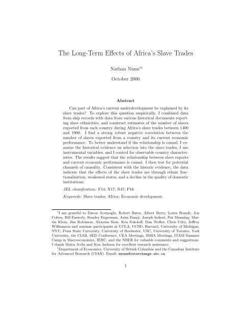
To illustrate the procedure that I use to combine the shipping data and
the ethnicity data to construct my estimates, I use an example, which is
shown in Figure 1. The figure is a hypothetical map of the western coast of
Africa.
Atlantic
Ocean
AFRICA
↑
N
100,000 ⇐
Country A Country B
250,000 ⇐
Country C
Country D
Country E
Figure 1: An Artificial Map of Africa’s West Coast
From the shipping data, I calculate the number of slaves shipped from
each coastal country in Africa. In the example, 100,000 slaves are shipped
from Country A and 150,000 are shipped from Country B. The problem
with relying on the shipping data alone is that many of slaves shipped from
Country A may have come from Country B, which lies landlocked behind
Country A. Using the ethnicity data, I construct the ratio of slaves from
each coastal country relative to the landlocked countries to the interior of
the coastal country. That is, I use the ethnicity data to determine the ratio
of slaves from Country A relative to Country B, and from Country C relative
to Countries D and E. Assume that the ratio of Countries A to B is 4 to
1, and Countries C to D and E is 3 to 1 to 1. Using the ratios I calculate
15

an estimate of the number of slaves shipped from the coast that came from
the inland country. For example, an estimated 100,000 × 1/5 = 20,000
slaves shipped from Country A are from Country B. Therefore, the estimate
number of slaves from Country B is 20,000 and from Country A is 80,000.
Using the same procedure yields estimates of 150,000 slaves from Country
C and 50,000 each from Countries D and E.
3.2 Measurement Error and Other Data Issues
There are a number of imperfections in the estimates that I have constructed.
First, the shipping data and the ethnicity data likely contain significant measurement
error. Slaves with similar but different ethnicities may have been
grouped together under one ethnicity. However, because I am aggregating
the data to the country level, this minimizes the bias introduced by ethnicity
mis-classification. The aggregation when moving from ethnicities to
countries can be seen in Figure 2, which maps African ethnicities based on
Murdock (1959), as well as modern political boundaries. As shown, ethnicities
are much finer than modern boundaries. Misclassification of slave
ethnicities will only cause measurement error if the falsely attributed ethnicity
is in a different country from the true ethnicity.
A second source of measurement error arises because slaves from the
interior are likely under-represented in the ethnicity samples. There are two
reasons for this. First, ethnicities originating inland sometimes, as they were
being shipped to the coast, adopted the language of the coastal ethnicities.
As a result, inland ethnicities may have then been grouped together with
coastal groups. Second, only slaves that survived the voyage outside of
Africa are in the ethnicity samples. The further inland a slave originated, the
longer the journey was, and the more likely it was that he or she died along
the way. Because of the high rates of mortality during the slave trades, this
form of measurement error may be significant. Estimates of cross-Atlantic
mortality rates ranged from 7 to 20% depending on the time period and
the length of the voyage (Curtin, 1969, pp. 275–286; Lovejoy, 2000, p. 63).
Death rates during the trek to the coast are known with less certainty, but
estimates range from 10 to 50% (Lovejoy, 2000, pp. 63–64; Vansina, 1990, p.
218). I show formally in Section A of the appendix that the under-sampling
of slaves from the interior results in OLS that are biased towards zero. In
addition, any random measurement error present in the data will have the
same effect. As well, one can use instruments that are uncorrelated with the
measurement error to derive consistent estimates. I do this in Section 5.2.
A final source of measurement error may arise because of my assumption
16

Figure 2: African ethnicities and current political boundaries. Source: Murdock
(1959).
17

Table 2: Total Slave Exports from Africa, 1400–1900
Slave Trade 1400–1599 1600–1699 1700–1799 1800–1900 1400–1900
trans-Atlantic 230,516 861,936 5,687,051 3,528,694 10,308,197
trans-Saharan 675,000 450,000 900,000 1,099,400 3,124,400
Red Sea 400,000 200,000 200,000 505,400 1,305,400
Indian Ocean 200,000 100,000 260,000 379,500 939,500
Total 1,505,516 1,611,936 7,047,051 5,512,994 15,677,497
that slaves shipped from a port within a country are either from that country
or from countries directly to the interior. Slaves shipped from a country’s
coast may have originated from a neighboring coastal country. In the data
appendix to the paper (Nunn, 2006a) I describe three different samples of
slaves from which one knows both the ethnicity of the slaves and the port
that they were shipped from. The three samples can be used to provide an
estimate of the precision of my estimating procedure. For each of the three
samples, my procedure would correctly identify the origins of 83.4, 84.9 and
97.6% of the slaves.
3.3 Data Summary
After the data have been constructed, I have estimates on the number of
slaves shipped from each country in Africa during each of the four slave
trades during four different time periods: 1400-1599, 1600-1699, 1700-1799,
1800-1900. 14 The data are summarized in Table 2. These estimates correspond
closely with the general consensus among African historians regarding
the total volume of slaves shipped in each slave trade. The only exception is
that the total exports for the trans-Atlantic slave trade are slightly less than
the standard estimate of 12 million slaves (e.g., Lovejoy, 2000). The lower
total is explained by the fact that the database only contains approximately
82% of all trans-Atlantic slaving voyages (Eltis and Richardson, forthcoming).
Table 3 reports the total number of slaves taken in the top exporting
countries. The estimates are consistent with the general view among
African historians of where the primary slaving areas were. During the
trans-Atlantic slave trade, slaves were taken in greatest numbers from the
Bight of Biafra (Benin and Nigeria), West Central Africa (Zaire and Angola),
14 Throughout the paper, I include Eritrea as part of Ethiopia.
18

Table 3: Total Slave Exports from 1400 to 1900 by Country.
Trans- Indian Trans- Red All
Atlantic Ocean Saharan Sea Slave Share
Country Trade Trade Trade Trade Trades of Total
Angola 3,616,027 0 0 0 3,616,027 23.1%
Nigeria 1,411,758 0 555,796 59,337 2,026,891 12.9%
Ghana 1,603,335 0 0 0 1,603,335 10.2%
Ethiopia 0 0 813,899 633,357 1,447,256 9.2%
Mali 524,102 0 509,950 1,034,052 6.6%
Sudan 615 0 408,260 454,913 863,788 5.5%
Dem. Rep. of Congo 752,828 0 0 0 752,828 4.8%
Mozambique 382,337 274,024 0 0 656,402 4.2%
Chad 823 0 409,367 118,673 528,863 3.4%
Tanzania 10,834 507,595 0 0 518,429 3.3%
Benin 461,782 0 0 0 461,782 2.9%
Senegal 222,359 0 98,732 0 321,091 2.0%
Togo 280,842 0 0 0 280,842 1.8%
Guinea 242,691 0 0 0 242,691 1.5%
and the Gold Coast (Ghana). All of these countries appear amongst the top
exporting countries on the list. Ethiopia and Sudan are also among the top
exporting countries. They were the primary sources of slaves shipped during
the Red Sea and Saharan slave trades. As well, the relative magnitudes of
exports from geographically close countries are consistent with the qualitative
evidence from the African history literature. Manning (1983, p. 839)
writes that “some adjoining regions were quite dissimilar: Togo exported
few slaves and the Gold Coast many.” The estimates are consistent with
Manning’s observation. Exports from Togo are far less than from Ghana.
4 Basic Correlations: OLS Estimates
I begin by testing for a relationship between past slave exports and current
economic performance. To do this, I use the following estimating equation
ln y i = β 0 + β 1 lnexports i + β 2 lnsize i + C ′ iδ + ε i (1)
where ln y i is the natural log of real per capita GDP in 2000; lnexports i
is the natural log of the total number of slaves exported between 1400 and
1900; lnsize i is a control for country size, either land area or population; and
C is a vector of dummy variables that indicate the origin of the colonizer
prior to independence, with the omitted category being for countries that
were not colonized.
OLS estimates of (1) are reported in Table 4. The first column reports
estimates without accounting for differences in the size of countries. In
19

column 2, I control for country size by the natural log of land area. An
alternative strategy is to normalize the number of slaves exported by land
area. This is done in column 3. In columns 4 and 5, I use the average
population of a country in every century between 1400 and 1900 as a measure
of country size. 15 The population data are from McEvedy and Jones (1978).
In columns 6 to 10, I re-estimate the specifications from columns 1 to 5,
except that indicator variables for the identity of the colonizer at the time
of independence are included in the regression equations. 16 In each of the
ten specifications, the slave export variables are negatively correlated with
subsequent economic development and they are statistically significant. The
results are independent of how one controls for country size and whether or
not the identity of the colonizer is controlled for.
The relationship between the natural log of slave exports normalized by
land area and the natural log of real GDP per capita in 2000 is shown in
Figure 3. In the raw data one observes a statistically significant negative
relationship between past slave exports and current income per capita. 17
Figure 4 shows the same graph with slave exports normalized by a country’s
average population between 1400 and 1900.
The partial regression plot for ln(exports/area) from the regression from
column 8 of Table 4 is shown in Figure 5. The plot shows that the relationship
is not driven by a small number of influential observations. I confirm
this with more formal sensitivity and robustness tests in Section 7.
The estimated magnitudes of the relationship between slave trades and
income are economically significant. The beta coefficients of the estimates
for ln(exports/area) range from −.45 to −.61. 18 If, for purely illustrative
purposes, one interprets the OLS estimates as causal, then according to the
column 8 estimate, for a country initially with the mean level of income of
$1,249, a one standard deviation decrease in the slave export variable will
raise income to $2,850.
One obtains similar results if average annual per capita GDP growth
between 1950 and 2000 is used as the measure of economic development.
15 I have also used the initial population in 1400, 1450 or 1500, or the post-slave trade
population in 1950 or 2000, as measures. Using any of these alternative population measures
produces similar results.
16 The results are robust if one uses alternative definitions of the colonizer for each
country. I have also used indicator variables for the identity of the colonizer on the eve of
World War I, rather than at independence. The results are nearly identical.
17 Because the natural log of zero is undefined, I take the natural log of .1. As I show in
Section 7, the results are robust to the removal of the zero slave export countries.
18 The beta coefficient is the change in the dependent variable, measured in standard
deviations, per one standard deviation change in the independent variable.
20

This is not surprising given that within Africa income levels in 2000 are
highly correlated with economic growth from 1950 to 2000. The correlation
between the two measures is .73.
21

Table 4: The Relationship between Income and Slave Exports. Dependent variable is ln real per capita GDP in
2000.
(1) (2) (3) (4) (5) (6) (7) (8) (9) (10)
22
ln(exports) −.076 ∗∗∗ −.091 ∗∗∗ −.070 ∗∗∗ −.078 ∗∗∗ −.091 ∗∗∗ −.094 ∗∗∗
(.019) (.025) (.025) (.017) (.050) (.025)
ln(exports/area) −.108 ∗∗∗ −.108 ∗∗∗
(.025) (.024)
ln(exports/pop) −.111 ∗∗∗ −.113 ∗∗∗
(.027) (.025)
ln(area) .058 .050
(.063) (.062)
ln(pop) −.033 .076
(.082) (.082)
Britain .370 .353 .354 .337 .319
(.483) (.486) (.481) (.485) (.485)
France .318 .312 .316 .318 .336
(.479) (.481) (.476) (.479) (.479)
Portugal .156 .218 .217 .219 .221
(.542) (.549) (.538) (.547) (.541)
Belgium −.980 −1.02 ∗ −.996 −1.14 ∗ −.999
(.600) (.604) (.597) (.624) (.602)
Spain 1.68 ∗∗ 1.69 ∗∗ 1.68 ∗∗ 1.70 ∗∗ 1.61 ∗
(.804) (.808) (.800) (.806) (.809)
U.N. 1.17 1.04 .896 1.21 1.16
(.780) (.814) (.802) (.798) (.797)
Italy .973 0.862 .732 .966 .935
(.789) (.804) (.790) (.791) (.791)
Number obs. 52 52 52 52 52 52 52 52 52 52
R 2 .25 .26 .27 .25 .25 .49 .50 .49 .50 .49
Notes: The dependent variable is the natural log of real per capita GDP in 2000. The slave export measures are the total
number of slaves exported from each country between 1400 and 1900 in the four slave trades. The colonizer variables are
indicator variables for the identity of the colonizer at the time of independence. Coefficients are reported with standard
errors in brackets. ∗∗∗ , ∗∗ , and ∗ indicate significance at the 1, 5, and 10 percent levels.

Relationship Between Current Income and Past Slave Exports
ln 2000 real per capita GDP
5 7.5 10
MUS
GNQ
SYC
BWA TUN
NAM
MAR SWZ
CPV
LSO
STP
DJI
RWA
BDI COM
ZAF
EGY
LBY
ZWE
UGA
CAF
(beta coef = −.52, t−stat = 4.30)
GAB
DZA
COG
MOZ SEN
CIV
BENGHA
CMR
NGA
KEN MRT SDN
SOM LBR
BFA MLI
GMB
AGO
ZMB
MDG MWI GNB
ETH
GIN TGO
NER
TZA
TCD
SLE
ZAR
−4 0 5 11
ln (exports/area)
Figure 3: Raw data: ln real per capita GDP in 2000 and ln slave exports
normalized by land area, ln(exports/area).
Relationship Between Current Income and Past Slave Exports
ln 2000 real per capita GDP
5 7.5 10
MUS
GNQ
SYC
TUN BWA
SWZ MAR
CPV
LSO
STP
DJI
RWA
COM BDI
EGY
UGA
ZAF
NAM
ZWE
CAF
(beta coef = −.50, t−stat = 4.11)
GAB
DZA
LBY
COG
MOZ SEN
CIV
BENGHA
CMR NGA
KEN SDN MRT
LBRSOM
BFA GMB
MLI
AGO
ZMB
MDG MWI GNB
ETH
GIN TGO
NER
TZA
TCD
SLE
ZAR
2 9 16
ln (exports/pop)
Figure 4: Raw data: ln real per capita GDP in 2000. and ln slave exports
normalized by population, ln(exports/pop).
23

Partial Correlation Plot: Current Income and Past Slave Exports
E(ln 2000 real per capita GDP | X)
−1.7 0 2.5
SYC
TUN
BWA
MAR
SWZ
CPV
LSO
STP
DJI
COM
MUS
ZAF
EGY
RWA
DZA
GAB
COG
(beta coef = −.53, t−stat = −4.77)
BDI
MOZ
LBR
SEN
CIV
BEN
ZWE
NAM GNQ LBY
CMR
GHA
MRT ETH
NGA
KEN SDN
BFA MLI AGO
CAF UGA
SOM
GMB
GNB
MDG
ZMB
MWI
GIN TGOZAR
NER
TZA
TCD
−7 0 8
E(ln (exports/area) | X)
SLE
Figure 5: Partial correlation plot: ln real per capita GDP in 2000 and
ln(exports/area), controlling for the identity of the colonizer.
24

5 Econometric Issues: Causality and Measurement
Error
Although the OLS estimates show that there is a relationship between slave
exports and current economic performance, it remains unclear whether the
slave trades have a causal impact on current income. An alternative explanation
for the relationship is that societies that initially had poor domestic
institutions or were frequently engaged in conflict and warfare may have
selected into the slave trades. These characteristics may persist today, adversely
affecting current income. Therefore, one observes a negative relationship
between slave exports and current economic development even though
the slave trades did not have a causal effect on subsequent development.
I pursue three strategies in order to evaluate the causal effect of the slave
trades. First, using historic data and qualitative evidence from African historians,
I evaluate the importance and characteristics of selection into the slave
trades. As I will show, the available evidence suggests that selection was important,
but that it was the societies that were initially the most prosperous,
not the most backward, that selected into the slave trades. Therefore, the
strong relationship between slave exports and current income cannot be explained
by selection. Rather, selection will bias the OLS estimates towards
zero. Second, I use the distance from each country to the location of the
demand for slaves to identify variation in slave exports that is uncorrelated
with any African characteristics. Third, I control for observable country
characteristics.
5.1 Historical Evidence on Selection during the Slave Trades
A large proportion of the early trade between Africans and Europeans was
also in commodities other than slaves. During this time, only societies with
institutions that were sufficiently developed were able to facilitate trade
with the Europeans. Between 1472 and 1483, the Portuguese sailed south
along the West coast of Africa, testing various points of entry looking for
trading partners. They were unable to find any societies north of the Zaire
river that could support trade. Vansina (1990, p. 200) writes that “the
local coastal societies were just too small in terms of people and territory;
their economic and social institutions were too undifferentiated to facilitate
foreign trade.” Sustained trade did not occur until the Portuguese found
the Kongo Kingdom, located just south of the Zaire river. Because the
Kongo Kingdom had a centralized government, national currency, and welldeveloped
markets and trading networks, it was able to support trade with
25

Initial Population Density and Subsequent Slave Exports
Initial Population Density and Subsequent Slave Exports
ln (exports/area)
0 10
NAM
STP SYC MUS COM CPVBWA
MRT
LBY
ZMB
ZAF
GAB
TCD
COG
NER
SWZ
DZA
CAF
DJI LSO
AGO
MLIMOZ
ZWE
MDG
SOM
LBR
CIV
GNB
SEN
ETH MWI
GIN
BFA
TZA
SDN ZAR
KENCMR
GNQ
GHA
TGO
BEN
MAR
EGY
(beta coef = .37, t−stat = 2.79)
NGA
GMB
SLE
UGA
TUN
RWA BDI
ln (exports/pop)
4 16
NAM
STP SYC MUS COM CPVBWA
MRT
LBY
ZMB
ZAF
GAB
CAF
COG
DZA
NER
SWZ
TCD
MLI
ZWE
DJI LSO
AGO
MOZ
MDG
SOM
GNB GHA
BEN TGO
ETH
SEN
GIN MWI
SDN TZA
GMBNGA
ZAR BFA
SLE
LBR
CIV
KENCMR
GNQ
MAR
EGY
(beta coef = .25, t−stat = 1.80)
UGA
TUN
RWA BDI
−2.5 0 3.5
ln population density in 1400
−2.5 0 3.5
ln population density in 1400
Figure 6: Left: ln population density in 1400 and ln(exports/area). Right:
ln population density in 1400 and ln(exports/pop).
the Europeans.
When European demand turned almost exclusively to slaves, the preference
to trade with the most developed parts of Africa continued. Because
the more prosperous areas were also the most densely populated, large numbers
of slaves could be efficiently obtained if civil wars or conflicts could be
instigated (Inikori, 2003, p. 182). As well, societies that were the most violent
and hostile, and therefore least developed, were often best able to resist
the European’s efforts to purchase slaves. For example, the slave trade in
Gabon was limited because of the defiance and violence of its inhabitants
towards the Portuguese. This resistance continued for centuries, and as a
result the Portuguese were forced to concentrate their efforts along the coast
further south (e.g., Hall, 2005, pp. 60–64).
Using data on initial population densities, I check whether it was the
more prosperous or less prosperous areas that selected into the slave trades.
Acemoglu et al. (2002) have shown that population density is a reasonable
indicator of economic prosperity. Figure 6 shows the relationship between
the natural log of population density in 1400 and the natural log of total
slave exports from 1400 to 1900 normalized by either land area or average
population from 1400 and 1900.
The data confirm the historical evidence on selection during the slave
trades. Figure 6 shows that the parts of Africa that were the most prosperous
in 1400, measured by population density, tend to also be the areas that were
26

most impacted by the slave trades.
A second potential source of selection may be that societies that initially
had domestic slavery may have selected into the slave trades. If this is the
case, then the estimates may be capturing a negative relationship between
domestic slavery and subsequent economic development similar to that documented
by Engerman and Sokoloff (1997, 2002), Sokoloff and Engerman
(2000) and Lagerlöf (2005).
For the areas of Africa that were a part of the much older Islamic slave
trades there was domestic slavery. It is unclear whether domestic slavery
is a cause or a consequence of the external slave trades. However, for the
parts of Africa that were previously untouched by the Islamic trades, recent
evidence shows that prior to the trans-Atlantic slave trade, chattel slavery
did not exist. 19 Hilton (1985) shows that in West Central Africa there was
no trade in people prior to the arrival of the Portuguese. She provides
evidence showing that in the sixteenth century, words that originally meant
‘servant’ or ‘prisoner’, were altered to take on the meaning of a traded slave.
Historian and Anthropologist Jan Vansina (1989), using much more detailed
linguistic data, confirms Hilton’s finding that in West Central Africa there
was no word previously for slave. Vansina also maps the origin of the word
‘pika’ which originally meant servant, but took on the meaning of a traded
slave. The word originated at the coastal ports engaged in the slave trade
and spread to the inland communities that were also involved in the trade
(see Vansina, 1989, 1990). Additional studies from other regions also show
that prior to the external slave trade domestic slavery did not exist (e.g.,
Harms, 1981; Inikori, 2000; Hall, 2005, p. 16).
5.2 Instrumental Variables
There are two potential sources of bias in the OLS estimates. One arises
from the existence of country characteristics that are correlated with both
slave exports and current economic performance. The other is the presence
of classical and non-classical measurement error in the slave export estimates.
A potential solution to the two problems is the use of instrumental
variables. If one can find instruments that are correlated with slave exports,
but uncorrelated with country characteristics and measurement error, then
instrumental variables will yield consistent estimates. In the following two
sections, I provide IV estimates using two different instrumenting strategies.
19 Before this evidence was brought forth, there was debate in the literature over whether
domestic slavery existed prior to European arrival (e.g., Fage, 1962; Rodney, 1970).
27

5.2.1 Distance to External Slave Markets
The first set of instruments that I use are the distances from each country to
the locations of where slaves were demanded. The validity of the instruments
relies on the presumption that although the location of demand influenced
the location of supply, the location of supply did not influence the location
of demand. For example, if sugar plantations began in the West Indies
because the West Indies were close to the western coast of Africa, then the
instruments are not valid. However, if instead many slaves were taken from
Western Africa because it is relatively close to the plantation economies in
the West Indies, then the instruments are valid.
According to the known history of slavery and the slave trades, it was the
location of demand that influenced the location of supply and not vice versa.
The location of the demand for African slaves was determined by a number
of factors, all unrelated to the supply of slaves. An important factor was
the location of climate and soil conditions suitable for plantation agriculture
using slave labor. In the West Indies, Mauritius, and the Southern United
States, slaves were imported because of climates suitable for growing highly
valued, globally traded commodities such as sugar and tobacco (Engerman
and Sokoloff, 1997, 2002; Sokoloff and Engerman, 2000). The existence of
gold and silver mines was a determinant of the demand for slaves in Brazil.
In the Northern Sahara, Arabia and Persia, slaves were needed to work in
salt mines, and in the Red Sea area slaves were used as pearl divers. An
area’s religion was also a determinant of the demand for slavery. In the
Muslim societies of North Africa and the Middle East, slaves were used as
eunuchs, concubines, soldiers, government officials, and servants.
Conceptually, the instruments measure the distance from the interior of
each country to the most important destinations in each of the four slave
trades. In practice, the following five instruments are used:
1. The overland distance from the centroid of a country to the closest
point along the coast. 20
2. The sailing distance from the point on the coast that is closest to the
country’s centroid to the closest major market of the Atlantic slave
trade. I use the nine largest importers of slaves, which are: Virginia,
20 Because sailing distances are from the point on the coast closest to each country’s
centroid, a country that lies inland of another country will not have the same sailing
distance as the coastal country. For the two countries the point on the coast that is
closest to each country’s centroid will be different.
28

USA; Havana, Cuba; Haiti; Kingston, Jamaica; Dominica; Martinique;
Guyana; Salvador, Brazil; and Rio de Janeiro, Brazil. 21
3. The sailing distance from the point on the country’s coast that is
closest to its centroid to the closest of the two major slave destinations
of the Indian Ocean slave trade: Mauritius and Muscat, Oman.
4. The overland distance from a country’s centroid to the closest port of
export for the trans-Saharan slave trade. The markets are: Algiers,
Tunis, Tripoli, Benghazi and Cairo.
5. The overland distance from a country’s centroid to the closest port of
export for the Red Sea slave trade. The ports are: Massawa, Suakin,
and Djibouti. 22
The distance instruments are also illustrated in Figure 7, which shows
the five distances for Burkina Faso. Also shown are the locations of demand
in each of the four slave trades. In the figure the ports and distance for
each of the slave trades is shown in a different color. Further details of the
construction of the instruments is given in the appendix.
Of the five instruments, there is particular concern that the distance
from a country’s interior to the coast is correlated with the error term in
the second stage. It has been shown that easy access to the coast allows
countries to more cheaply engage in international trade, which increases income
(see Rappaport and Sachs, 2003). In addition, distance to the coast is
correlated with the measurement error that results from the under-sampling
of slaves from the interior. Even though the distance to the coast is problematic
as an instrument, it is still useful to report the estimates with the
variable included as part of the instrument set. As I show in Section B of the
appendix, if the instrument is positively correlated with the measurement
error and/or negatively correlated with the error term in the second stage,
then the IV estimate will be biased towards zero. Therefore, the IV estimate
with distance to the coast in the instrument set is still useful because it can
be taken as a lower bound estimate of the effect of slave exports on income.
I also report estimates after eliminating the distance to the coast variable
from the instrument set.
21 Data on slave imports are from Eltis and Richardson (forthcoming). There is a significant
drop in the volume of slave imports between the 9th and 10th largest markets.
Because of this natural break, I use the top 9 markets.
22 For the island countries, one cannot reach the ports of the Saharan or Red Sea slave
trades by traveling overland. For these countries I use the sum of the sailing distance and
overland distance.
29

Figure 7: Example showing the distance instruments for Burkina Faso.
Table 5 reports the IV estimates. In columns 1 and 4, I report the OLS
estimates, with and without colonial controls, for comparison. In columns 2,
3, 5, and 6, the IV estimates are reported. The first stage coefficients for the
instruments are negative as expected, suggesting that if a country is further
from slave markets, then less slaves are exported. All coefficients, except for
the distance from each country’s centroid to the coast and distance to the
Red Sea ports, are statistically significant.
In the second stage, the estimated coefficient for ln(exports/area) remains
significant and negative. Because the first stage F-statistics are low, I
report Anderson-Rubin confidence intervals. In all specifications the magnitudes
of the IV estimates are larger than the corresponding OLS estimates.
This is expected given the classical and non-classical measurement errors in
the slave exports variable, and the selection of the initially most prosperous
societies into the slave trades, both of which result in OLS estimates that
are biased downwards. If the instruments satisfy the necessary exclusion
restrictions and are uncorrelated with both sources of measurement error,
then the IV estimates will be larger in magnitude than the OLS estimates.
30

Table 5: IV Estimates Using Distances to the Locations of Demand as
Instruments.
OLS IV IV OLS IV IV
(1) (2) (3) (4) (5) (6)
Second Stage. Dependent variable is log income in 2000
ln(exports/area) −.108 ∗∗∗ −.182 ∗∗∗ −.192 ∗∗∗ −.108 ∗∗∗ −.185 ∗∗∗ −.188 ∗∗∗
(−.025) [−.61, −.17] [−.48, −.14] (.024) [−.63, −.10] [−.52, −.11]
Colonizer fixed effects No No No Yes Yes Yes
F-stat 18.5 11.9 12.6 5.22 4.16 4.14
Number obs. 52 52 52 52 52 52
First Stage. Dependent variable is ln(exports/area)
Interior distance −.0006 −.0007
(.0014) (.0016)
Atlantic distance −.0012 ∗∗∗ −.0011 ∗∗∗ −.0016 ∗∗∗ −.0015 ∗∗∗
(.0004) (.0004) (.0005) (.0004)
Indian distance −.0008 ∗∗∗ −.0008 ∗∗∗ −.0009 ∗∗ −.0009 ∗∗∗
(.0003) (.0003) (.0003) (.0003)
Saharan distance −.0019 ∗∗ −.0019 ∗∗ −.0021 ∗∗ −.0021 ∗∗
(.0008) (.0008) (.0009) (.0008)
Red Sea distance −.0004 −.0002 −.0008 −.0006
(.0008) (.0008) (.0009) (.0008)
Colonizer fixed effects No No Yes Yes
F-stat 3.33 4.19 2.08 2.30
Sargan test (p-value) .04 .09 .24 .19
Hausman test (p-value) .07 .04 .01 .01
Notes: Slave exports is the total number of slaves exported from each country between 1400 and
1900 in the four slave trades. The colonizer variables are indicator variables for the identity of the
colonizer at the time of independence. Coefficients are reported, with standard errors in brackets.
For the endogenous variable, Anderson-Rubin 95 percent confidence regions are reported rather
than standard errors. The p-value of the Hausman test is for the Wu-Hausman chi-squared test.
∗∗∗ , ∗∗ , and ∗ indicate significance at the 1, 5, and 10 percent levels.
31

Table 6: IV Estimates Using Initial Population Density as an Instrument.
OLS IV IV OLS IV IV
(1) (2) (3) (4) (5) (6)
Second Stage. Dependent variable is log income in 2000
ln(exports/area) −.112 ∗∗∗ −.199 ∗∗∗ −.168 ∗∗∗ −.104 ∗∗∗ −.113 ∗∗ −.116 ∗∗
(.026) [−.54, −.06] [−.34, −.06] (.025) [−.23, −.01] [−.22, −.02]
ln(2000 pop density) −.073 −.106 .043 .032
(.078) (.088) (.084) (.091)
Colonizer fixed effects No No No Yes Yes Yes
F-stat 9.64 6.71 4.22 6.76 3.35 3.42
Number obs. 52 52 52 52 52 52
First Stage. Dependent variable is ln(exports/area)
ln(1400 pop density) 1.09 ∗∗∗ 1.43 ∗∗∗ 1.65 ∗∗∗ 1.85 ∗∗∗
(.392) (.391) (.436) (.408)
ln(2000 pop density) −1.07 ∗∗∗ −1.23 ∗∗∗
(.401) (.091)
Colonizer fixed effects No No Yes Yes
F-stat 7.81 7.91 2.59 3.68
Hausman test (p-value) .14 .15 .88 .24
Notes: Slave exports is the total number of slaves exported from each country between 1400
and 1900 in the four slave trades. The colonizer fixed effects are seven indicator variables
for the identity of the colonizer at the time of independence. Coefficients are reported, with
standard errors in brackets. For the endogenous variable, Anderson-Rubin 95 percent confidence
regions are reported rather than standard errors. The p-value of the Hausman test is for the
Wu-Hausman chi-squared test.
∗∗∗ , ∗∗ , and ∗ indicate significance at the 1, 5, and 10 percent
levels.
32

5.2.2 Initial Population Density
The second IV strategy is to use initial population density as an instrument.
As shown in Section 5.1, slaves tended to be exported from areas with high
initial population densities. This suggests that population density is a possible
instrument for slave exports. However, it is unlikely that initial population
density satisfies the necessary exclusion restrictions. There are two
reasons for this. First, past population density will be positively correlated
with good initial characteristics of the country, which may persist, affecting
current income. However, this correlation, as I show in Section B of
the appendix, results in an IV estimate that is biased towards zero. Therefore,
the IV estimate can be taken as a lower bound estimate. Second, past
population density is correlated with current population density, which may
affect income directly. Herbst (2000) argues that low population densities
are responsible for Africa’s poor economic performance. Again, if this relationship
exists, then the IV estimate will be biased towards zero, and can
be taken as a lower bound estimate. I also control for current population
density in the second stage.
The IV results are reported in Table 6. In all specifications, the estimated
coefficient for the log of population density in 1400 is positive, as
expected, and statistically significant. The IV estimates for ln(exports/area)
are negative and larger in magnitude than the OLS estimates. In general,
these IV estimates are lower than the IV estimates when the distance to
slave markets (reported in Table 5) are used. This is consistent with the
population density IV estimates being biased towards zero and therefore
being lower bound estimates.
5.3 Controlling for Additional Country Characteristics
The third strategy is to control for additional country characteristics that
may affect income per capita, and therefore bias OLS estimates, if omitted
from the regression equations. The results are reported in Table 7. In the
first column, I add to the estimating equation five region fixed effects: Central
Africa, Western Africa, Southern Africa, Eastern Africa, and Northern
Africa. The fixed effects control for any country characteristics that differ
by region.
I also include variables that control for differences in countries’ physical
environment, endowments of natural resources, culture, and religion.
In columns 2 to 4, I control for a country’s geographic environment, by
including distance to the equator, natural openness measured by the log
33

Table 7: Income and slave exports, adding control variables. Dependent
variable is ln real per capita GDP in 2000.
(1) (2) (3) (4) (5) (6) (7) (8)
ln(exports/area) −.093 ∗∗∗ −.091 ∗∗∗ −.077 ∗∗∗ −.120 ∗∗∗ −.083 ∗∗∗ −.090 ∗∗∗ −.102 ∗∗∗ −.094 ∗∗∗
(.030) (.030) (.028) (.028) (.031) (.029) (.025) (.029)
Absolute latitude .012 .022 ∗∗ .014
(.020) (.010) (.018)
ln(coastline/area) .108 ∗∗∗ .089 ∗∗∗ .069 ∗
(.038) (.027) (.036)
ln(gold prod/pop) −.006 −.001 .006
(.018) (.017) (.017)
ln(oil prod/pop) .118 ∗∗∗ .089 ∗∗∗ .087 ∗∗∗
(.031) (.022) (.030)
ln(diamonds prod/pop) .017 −.015 .001
(.047) (.042) (.046)
% Christian .002 −.007 .002
(.006) (.005) (.006)
% Islamic .006 −.010 ∗∗ −.005
(.005) (.004) (.005)
French legal origin .879 ∗ −.238 .652
(.457) (.187) (.437)
Colonizer fixed effects Yes Yes Yes Yes Yes Yes No Yes
Region fixed effects Yes Yes Yes Yes Yes Yes No Yes
Number obs. 52 52 52 52 52 52 52 52
R 2 .53 .54 .62 .67 .59 .58 .63 .77
Notes: The dependent variable is the natural log of real per capita GDP in 2000. Slave exports is the total
number of slaves exported from each country between 1400 and 1900 in the four slave trades. The colonizer
fixed effects are seven indicator variables for the identity of the colonizer at the time of independence. The
omitted category is for countries that were not colonized. Coefficients are reported with standard errors in
brackets. ∗∗∗ , ∗∗ , and ∗ indicate significance at the 1, 5, and 10 percent levels.
34

of coastline divided by land area, and countries’ endowments of gold, diamonds,
and oil, measured by the natural log of average production per
capita between 1970 and 2000. In columns 5 and 6, I include measures of
countries’ cultural characteristics. I control for the fraction of a country’s
population that is Christian, the fraction that is Muslim, and for a country’s
legal origin. In the final two columns, I include all of the control variables
together, without and with the region fixed effects and colonizer fixed effects.
23 In every specification, the coefficient of the slave exports variable
remains negative and statistically significant. 24
6 Examining Potential Channels of Causality
Given that the evidence suggests that the relationship between the slave
trades and current economic performance is causal, I now turn to the potential
channels through which the slave trades may affect economic development.
Motivated by the research of African historians, I test the potential
channels of causality summarized in Section 2.2. The most likely channels
are subsequent state development, ethnic fractionalization, and the quality
of domestic legal institutions.
When examining the effect that slave exports have on these factors, the
question of causality remains important. If one finds a relationship in the
data, it is unclear whether the slave trades affected this measure or whether
the slave trades and the measure are both correlated with unobserved country
characteristics. Here, I use the same instrumenting strategy that I used
when considering the slave trade-income relationship. I use the distance
from each country to the locations of demand for slaves as instruments.
As I have shown, these measures were an important determinant of slave
exports. More importantly, they are likely uncorrelated with initial characteristics
of African countries that may affect subsequent state development,
institutional change, or ethnic fractionalization, except through their impact
on slave exports.
In Table 8, I report IV and OLS estimates of the relationship between
slave exports and variables that measure the different channels of causality.
23 The only control variables that are consistently significant are the production of oil
and the log of the coastline divided by land area. These results are consistent with previous
studies finding that oil production increases income (e.g., Easterly and Levine, 2003), and
that natural openness increases income (e.g., Rappaport and Sachs, 2003).
24 Although not reported here, the results also remain robust to the inclusion of additional
geographic measures, such as elevation, temperature, humidity, rainfall, and frost
days. The data are from Parker (1997).
35

I first test whether slave exports are correlated with the level of domestic
state development after the slave trades, but prior to colonial rule. The measure
of pre-colonial state development is from Gennaioli and Rainer (2005).
The authors construct the measure using ethnographic data from Murdock
(1967) on the indigenous political complexity of ethnic groups, measured by
the number of jurisdictional hierarchies beyond the local community. The
original measure ranges from 0 to 4, with 0 indicating “stateless” societies
and 4 indicating societies with “large states” (Murdock, 1967, p. 52). Using
this data, Gennaioli and Rainer (2005) construct a measure of the proportion
of a country’s indigenous population that belongs to an ethnic group
that has 0 or 1 jurisdictional hierarchies beyond the local community. The
variable provides a measure of how developed a country’s indigenous states
were prior to colonization. According to both the OLS and IV estimates, the
slave trades are negatively correlated with state development. This result
supports the research of African historians suggesting that the slave trades
resulted in political instability and fragmentation. In all specifications the
relationship is significant, although the significance is marginal for the IV
estimates without colonizer fixed effects.
In the second row of the table, I consider the relationship between slave
exports and a measure of current domestic legal institutions using an index
of each country’s rule of law in 2000 from Kaufmann et al. (2003). The estimates
suggest that slave exports are negatively correlated with the quality
of the rule of law in 2000, a result that is consistent with previous historical
research. Next, I consider the possibility that the slave trades also
caused ethnic and social fractionalization, which persists today. I use two
variables to capture this channel. The first is a measure of ethnic fractionalization
from Easterly and Levine (1997). The second is a measure of cultural
diversity from Fearon (2003). Cultural diversity is a measure of ethnic fractionalization
that also takes into account the cultural distance between the
ethnicities of a country. Both measures are strongly correlated with slave
exports, which is consistent with the view that the slave trades impeded
political and social development, causing ethnically fragmented societies. 25
The last row of the table reports the relationship between slave exports
and income per capita in 1950. As shown, the relationship between slave exports
and income in 1950 is negative, but weak. This result provides insight
into the channels through which the slave trades operate. As discussed, the
25 The results are similar if other measures of fractionalization are used. For example,
using the other measures constructed by Fearon (2003) or measures from Alesina et al.
(2003) yield very similar results.
36

Table 8: Testing potential channels of causality.
Without colonizer fixed effects With colonizer fixed effects
OLS IV OLS IV
coef s.e. coef s.e. coef s.e. coef s.e.
Dependent variable
Pre-colonial state dev. −.026 ∗∗ (.013) −.069 ∗∗∗ (.025) −.026 ∗ (.015) −.064 ∗∗ (.025)
Rule of law −.073 ∗∗∗ (.020) −.118 ∗∗∗ (.039) −.078 ∗∗∗ (.018) −.095 ∗∗∗ (.032)
Ethnic fractionalization .040 ∗∗∗ (.009) .065 ∗∗∗ (.018) .041 ∗∗∗ (.010) .066 ∗∗∗ (.019)
Cultural diversity .029 ∗∗∗ (.007) .050 ∗∗∗ (.014) .031 ∗∗∗ (.008) .051 ∗∗∗ (.014)
ln per capita GDP in 1950 −.026 (.020) −.058 (.038) −.030 (.021) −.062 (.037)
Notes: The coefficients and standard errors reported are for ln(exports/area). In the IV regressions,
the instruments are the four distances to the markets of demand in each of the four slave trades.
The colonizer fixed effects are indicator variables for the identity of the colonizer at the time of
independence. Coefficients are reported with standard errors in brackets.
∗∗∗ , ∗∗ , and ∗ indicate
significance at the 1, 5, and 10 percent levels.
effects of the slave trades may be through state development, domestic institutions,
or ethnic fractionalization, which is an important determinant of
domestic policies such as the provision of public goods. In 1950, nearly all
countries were still under colonial rule, and therefore a country’s domestic
institutions and policies were externally imposed. 26 If the slave trades affect
income through the development of domestic institutions and policies, then
we would expect the relationship between the slave trades and income to be
much weaker, or even non-existent, when a country’s institutions and policies
are determined externally by a colonial power. The weak relationship
between slave exports and 1950 income is consistent with this. 27
7 Robustness and Sensitivity Analysis
The first set of tests that I perform check the robustness of my results to
the construction of the slave export data. As I noted in Section 3, the data
used to construct the slave export estimates for the Saharan, Indian Ocean
26 In 1950 only four African countries were independent. Ethiopia had never been colonized,
while Liberia, South Africa, and Egypt had gained independence.
27 An alternative way of expressing this is that income in 1950 may not be a good
indicator of a country’s economic development at that time. High income may simply
reflect high levels of extraction by the colonizer rather than a good economic environment.
37

Table 9: Robustness to Data Construction. Dependent variable is ln real
per capita GDP in 2000.
Without colonizer With colonizer
fixed effects
fixed effects
coef s.e. R 2 coef s.e. R 2
Baseline −.108 ∗∗∗ (.025) .27 −.108 ∗∗∗ (.024) .49
Saharan exports set to zero −.052 ∗∗∗ (.013) .26 −.058 ∗∗∗ (.011) .53
Indian Ocean exports set to zero −.049 ∗∗∗ (.014) .20 −.055 ∗∗∗ (.012) .49
Red Sea exports set to zero −.048 ∗∗∗ (.014) .19 −.055 ∗∗∗ (.012) .48
Atlantic exports set to zero −.026 ∗ (.014) .07 −.032 ∗∗ (.014) .33
Atlantic exports only −.065 ∗∗∗ (.021) .16 −.067 ∗∗∗ (.020) .41
Notes: The dependent variable is the natural log of real per capita GDP in 2000. The
colonizer fixed effects are indicator variables for the identity of the colonizer at the time
of independence. Coefficients are reported with standard errors in brackets.
∗∗∗ , ∗∗ ,
and ∗ indicate significance at the 1, 5, and 10 percent levels.
and Red Sea slave trades are of lower quality than the data used for the
trans-Atlantic slave trade. Here I show that the results do not depend on
the slave export estimates that are based on less precise data sources. This
is shown in Table 9. In the first row, for comparison I report the baseline
estimates without and with the colonizer fixed effects. In the second row, I
recalculate my measure of total slave exports, setting slave exports from the
Saharan slave trade to zero. This would be the preferred measure of total
slave exports if one felt that the data from the Saharan slave trade were too
unreliable to be used. Using the new measure, I re-estimate my baseline
specifications. The third and fourth rows report the results when the Indian
Ocean and Red Sea slave exports are set to zero. In all six of the specifications
reported in rows 2 to 4, the estimated coefficient remains negative
and statistically significant. Next, I recalculate my total slave exports figure
after setting trans-Atlantic slave exports to zero. The estimated coefficient
remains negative, but it is now only marginally significant. In the final row,
I report the estimated coefficient if I use trans-Atlantic slave exports as my
measure of total slave exports. That is, I simultaneously set slave exports
in the Saharan, Red Sea and Indian Ocean slave trades to zero. The coefficient
remains negative and is highly significant. These results show that the
importance of total slave exports is primarily driven by the trans-Atlantic
slave trade, and that the results are robust to using only the most precise
38

Table 10: Robustness and Sensitivity Checks. Dependent variable is ln real
per capita GDP in 2000.
Without colonizer fixed effects With colonizer fixed effects
Omitted Observations coef s.e. N R 2 coef s.e. N R 2
None −.108 ∗∗∗ (.025) 52 .27 −.108 ∗∗∗ (.024) 52 .49
South Africa −.105 ∗∗∗ (.025) 51 .26 −.104 ∗∗∗ (.024) 51 .49
North African countries −.097 ∗∗∗ (.027) 47 .23 −.096 ∗∗∗ (.025) 47 .47
Island countries −.104 ∗∗∗ (.026) 47 .26 −.110 ∗∗∗ (.025) 47 .55
All of the above −.078 ∗∗∗ (.028) 41 .17 −.079 ∗∗∗ (.027) 41 .53
Zero export countries −.139 ∗∗∗ (.037) 39 .28 −.087 ∗∗ (.043) 39 .51
|ê i| > 2.0 −.103 ∗∗∗ (.022) 47 .33 −.109 ∗∗∗ (.021) 48 .56
|ê i| > 1.8 −.106 ∗∗∗ (.021) 46 .36 −.109 ∗∗∗ (.027) 48 .56
|ê i| > 1.5 −.096 ∗∗∗ (.021) 45 .33 −.101 ∗∗∗ (.020) 46 .58
|ê i| > 1.0 −.099 ∗∗∗ (.018) 35 .48 −.102 ∗∗∗ (.016) 35 .79
dffits −.105 ∗∗∗ (.021) 44 .37 −.108 ∗∗∗ (.022) 49 .53
Cook’s Distance −.108 ∗∗∗ (.023) 48 .32 −.108 ∗∗∗ (.024) 51 .47
Welsch Distance −.088 ∗∗∗ (.024) 50 .22 −.108 ∗∗∗ (.024) 51 .47
Notes: The dependent variable is the natural log of real per capita GDP in 2000. The
colonizer fixed effects are indicator variables for the identity of the colonizer at the time
of independence. Coefficients are reported with standard errors in brackets. ∗∗∗ , ∗∗ , and ∗
indicate significance at the 1, 5, and 10 percent levels. Influential variables were omitted
using the following standard rules. dffits: omit if dffits i > 2 √ k/n. Cook’s distance:
omit if Cook’s distance > 4/n. Welsch distance: omit if Welsch distance > 3 √ k. n is the
number of observations and k is the number of independent variables.
39

data to construct the total slave export estimates.
I perform additional sensitivity and robustness tests, which are summarized
in Table 10. In the first panel of the table, I re-estimate my equations
after omitting countries that may be different from the rest of the sample.
It is possible that the results are being driven by a group of countries with
peculiar characteristics that are unrelated to the slave trades. The first row
of the table reports the baseline estimates for comparison. In the second
row, I re-estimate my equations after omitting South Africa from the sample.
Because this country has a large number of European settlers, economic
performance may be different from other African countries for reasons unrelated
to the slave trades. I repeat this procedure, omitting North African
countries and omitting Island countries. In the fifth row, I simultaneously
omit South Africa, North African countries, and Island countries. In the
final row, I omit all countries with zero slave exports. For all specifications
the coefficient for slave exports remains negative and statistically significant.
In the second and third panels of the table, I more formally identify
potentially influential observations and check whether the results are driven
by these. In the second panel, I re-estimate my baseline equations after
sequentially omitting observations with ‘studentized’ residuals greater than
2.0, 1.8, 1.5, and 1.0. 28 In the third panel of the table, I identify influential
observations using three rules that have been proposed in the literature
(Belsley et al., 1980; Welsch, 1982). Using each rule, I omit the observations
identified as outliers and re-estimate my estimating equations. In every
estimation, the results remain robust.
8 Conclusions
Combining data from shipping records and data from historical records reporting
slave ethnicities, I have constructed estimates of the number of slaves
exported from each country in Africa between 1400 and 1900. I found a robust
negative relationship between the number of slaves taken from a country
and its subsequent economic development.
I pursued three strategies to better understand if the relationship is
causal or spurious. Countries initially with poor characteristics may have
selected into the slave trades and these poor characteristics may persist
28 Studentized residuals are calculated from a regression line that is fitted with the observation
in question removed from the sample. This avoids the problem of an outlier
influencing the estimated regression line, resulting in underestimated residual for the observations.
40

causing current underdevelopment. I first reviewed the historical evidence
on the characteristics of African societies that were most affected by the slave
trades. The qualitative and quantitative evidence show that it was actually
the most developed parts of Africa, not the least developed, that tended to
select into the slave trades. I also used instrumental variables to estimate
the causal effect of the slave trades on subsequent economic development.
The main instruments I used were the sailing and overland distances from
each country to the closest locations of demand in each of the four slave
trades. Like the OLS estimates, the IV estimates are negative, suggesting
that increased extraction during the slave trades caused worse subsequent
economic performance. As a final strategy, I controlled for observable country
characteristics. These results also confirm that the slave trades had a
causal impact on subsequent economic development.
I then examined the precise channel of causality underlying the relationship
between slave exports and subsequent economic development. Using
historical evidence as a guide, I then examined whether slave exports resulted
in a fragmentation and weakening of states, ethnic fractionalization,
and a deterioration in the quality of judicial institutions. I found support
for the view that the slave trades resulted in weak, politically fragmented
states, ethnic fractionalization, and poor judicial institutions.
A Deriving the Bias from the Under-Sampling of
Slaves from the Interior
I show here that the non-classical measurement error present in the slave
export data will result in OLS estimates of the effect of slave exports on
income that are biased towards zero.
To see this, denote the true number of slaves taken from country i by
s ∗ i , the observed number of slaves by s i, distance to the coast by d i , and
economic development by y i . All variables are expressed as deviations from
means. Assume the true relationship between the number of slaves exported
and distance to the coast is given by
s ∗ i = −αd i + ε i (2)
where α > 0 and ε i is i.i.d. drawn from a normal distribution. The relationship
between the observed number of slaves exported s i and the distance to
the coast d i is given by
s i = s ∗ i − γd i + ν i (3)
41

where γ > 0 and ν i is uncorrelated with ε i . The true relationship between
slave exports and development is given by
y i = −βs ∗ i + ω i (4)
where β > 0 and ω i is uncorrelated with all other variables.
If one estimates y i = bs i + ξ i by OLS, then the estimated relationship
between s i and y i is
Substituting (2) into (3) gives
Similarly, (2) and (4) give
ˆb =
∑i s iy i
∑
i s2 i
(5)
s i = −(α + γ)d i + ε i + ν i (6)
y i = βαd i − βε i + ω i (7)
Substituting (6) and (7) into (5), and taking the plim of ˆb gives
[
plim ˆb σs 2 = −β
∗ + ]
γασ2 d
σs 2 ∗ + 2γ(α + γ)σ2 d + σ2 ν
(8)
where σ 2 s ∗ = α2 σ 2 d + σ2 ε.
First, consider the case when the only source of measurement error is
classical measurement error. Then γ = 0 and (8) reduces to the standard
formula for attenuation bias: plim ˆb = −β[σ 2 s ∗/(σ2 s ∗ + σ2 ν )].
Next, consider the measurement error introduced by the under-sampling
of slaves from the interior. The result of this is that the under-estimation
of slave exports is increasing in a country’s distance from the coast: γ > 0.
Looking at (8), it is apparent that 2γ(α+γ) > γα and therefore the presence
of non-classical measurement error also biases towards zero the estimated
coefficient, reinforcing the attenuation bias resulting from classical errorsin-variables.
Asymptotically, ˆb is biased even further towards zero because
of the under-sampling of slaves from the interior.
B Deriving the Bias of the IV Estimates
I now consider the potential bias introduced to IV estimates if the instruments
are correlated with the second stage error term, which may include
measurement error in the slave export variable.
42

B.1 Using Distance to Slave Markets as Instruments
Let the instrument be denoted by z i . I use the core equations presented in
the previous section, but make one change to allow the instrument to be an
additional determinant of the true number of slaves exported. Equation (2)
is replace with
s ∗ i = −α 1d i − α 2 z i + ε i (9)
Substituting (9) into (3) gives
and (9) and (4) give
s i = −(α 1 + γ)d i − α 2 z i + ε i + ν i (10)
y i = βα 1 d i + βα 2 z i − βε i + ω i (11)
If one estimates y i = bs i + ξ i by IV, using z i as an instrument, then the
estimated relationship between s i and y i is
∑
ˆbiv = ∑ i z iy i
i z (12)
is i
Substituting (10) and (11) into (12), and taking the plim of ˆb iv gives
[
plim ˆb α 2 σ 2 ]
z + α 1 σ zd
σ zω
iv = −β
α 2 σz 2 −
+ (α 1 + γ)σ zd α 2 σz 2 (13)
+ (α 1 + γ)σ zd
where I assume that the instrument is uncorrelated with the classical measurement
error (σ zν = 0).
If the instrument is uncorrelated with distance to the coast (σ zd = 0)
and if the instruments are valid (σ zω = 0), then ˆb iv is consistent. Now
consider an instrument that is positively correlated with distance to the
coast. Then σ zd > 0. As well, the instrument will be positively correlated
with transportation costs, which negatively affect income directly: σ zω < 0.
Then the term in the square bracket is positive and less than one, while the
term being subtracted is negative. Therefore, both the term in the square
brackets and the term being subtracted cause the IV estimate to be biased
towards zero (i.e., upwards): ˆb iv > −β 1 .
B.2 Using Initial Population Density as an Instrument
Next, consider initial population density as an instrument. Because this
instrument is positively correlated with slave exports, Equation 9 is replace
by
s ∗ i = −α 1d i + α 2 z i + ε i (14)
43

Following the exact same procedure as above yields the following expression
for the plim of ˆb iv
[
plim ˆb α 2 σ 2 ]
z − α 1 σ zd
σ zω
iv = −β
α 2 σz 2 +
− (α 1 + γ)σ zd α 2 σz 2 (15)
− (α 1 + γ)σ zd
If initial population density is uncorrelated with the distance to the coast
(and the non-classical measurement error), but is correlated with current
population density, which is positively correlated with current income, then
σ zd = 0 and σ zω > 0, and (15) reduces to
plim ˆb iv = −β + σ zω
α 2 σ 2 z
(16)
In this case, the IV estimate using initial population density as an instrument
is biased towards zero (i.e., upwards).
C
Data
Real per capita GDP in 1950 and 2000 are from Maddison (2003). Land
area, measured in millions of square kilometers, is from Parker (1997). Historic
population figures, measured in thousands of people, are from McEvedy
and Jones (1978). For some groups of the smaller countries of Africa, population
data are only disaggregated to a regional level. In these cases the
data are disaggregated to the country level using the distribution of population
in 1950 from the United Nations. Data on the identity of the colonizer
before independence are from the Political Regimes and Regime Transitions
in Africa, 1910–1994 data set (Bratton and van de Walle, 1997). The data
on the production of diamonds, crude petroleum, and mined gold are from
the British Geological Survey’s World Mineral Statistics and World Mineral
Production. All three variables are measured as the natural log of the
average annual production per thousand inhabitants from 1970 to 2000. Diamonds
include both gemstones and industrial diamonds and are measured
in thousands of carats. Crude Petroleum is measured in thousands of tonnes
and mined gold is measured in kilograms. Data on countries’ legal origins
are from La Porta et al. (1999). Ethnic fractionalization is from Easterly
and Levine (1997), and cultural diversity is from Fearon (2003). Data on
a country’s coastline, religion, and average latitude are from Parker (1997).
Countries’ total coastline is measured in kilometers. The religion variables
are the fraction of a country’s population that are Christian and Islamic.
Latitude is measured as the absolute value of the country’s average latitude
measured in degrees.
44

The rule of law in 2000 is from Kaufmann et al. (2003). It is an index
ranging from −2.5 to 2.5 that measures the extent to which agents have
confidence in and abide by the rules of society.
When taking the natural log of variables that may take on the value
of zero, I replace the zero observations with 1 × 10 n , where n is the largest
integer value possible subject to 1×10 n being less than the smallest non-zero
observation in the data.
The distance instruments measure the shortest sailing distances to the
location of demand in the trans-Atlantic and Indian Ocean slave trades, and
the shortest overland distance to the locations of demand in the Red Sea
and trans-Saharan slave trades. In practice, distances are calculated using
the great circle distance between two locations. The formula for this is:
d ij = arccos{sin(La i )sin(La j ) + cos(La i )cos(La j )cos(Lo i − Lo j )} × 111.12,
where d ij is the distance in kilometers between location i and j, La i is
the latitude of location i in degrees, and Lo i is the longitude of location
i in degrees. When calculating the sailing distances, I do not allow ships
to sail across land. 29 For example, for voyages from Northern Africa in
the trans-Atlantic slave trades, I calculate the sailing distance through the
Mediterranean sea and the Strait of Gibraltar to the closest market in the
Atlantic Ocean. For the distance from these countries in the Indian Ocean
slave trade, I calculate the sailing distance through the Mediterranean sea,
and then south around the Cape of Good Hope. Similarly, when calculating
distances from East African countries during the trans-Atlantic slave trade,
and for distances from West African countries during the Indian Ocean slave
trade, I calculated the sailing distance around the Cape of Good Hope.
The centroid of each country is calculated using the Centroid Utility in
ArcGIS. For five countries where the centroid falls outside the land borders
of the country (Gambia, Somalia, Cape Verde, Mauritius and Seychelles)
the point within the country closest to the centroid is used. The location
on the coast that is closest to each country’s centroid is identified using the
Proximity Utility in ArcGIS.
29 As well, I do not allow ships to sail through the Suez Canal since it was not completed
until 1869.
45

Table 11: Summary Statistics of Main Variables
Variable Mean std. dev. Min Max N
ln real per capita GDP in 2000 7.13 .83 5.38 9.27 52
ln(exports/area) 3.12 3.98 −2.30 8.81 52
ln(exports/pop) 9.17 3.73 3.91 14.40 52
Rule of law 2000 −.55 .70 −1.97 1.14 52
Pre-colonial state dev. .54 .32 0 1 42
Ethnic fractionalization .57 .31 0 1 52
Cultural diversity .40 .21 0 .21 48
ln real per capita GDP in 1950 6.65 .57 5.67 8.04 52
46

References
Acemoglu, Daron, “Reward Structure and the Allocation of Talent,” European Economic
Review, 39 (1995), 17–33.
———, “Politics and Economics in Weak and Strong States,” Journal of Monetary Economics,
52 (2005), 1199–1226.
Acemoglu, Daron, and Simon Johnson, “Unbundling Institutions,” Journal of Political
Economy, 113 (2004), 949–995.
Acemoglu, Daron, Simon Johnson, and James A. Robinson, “The Colonial Origins of
Comparative Development: An Empirical Investigation,” American Economic Reivew,
91 (2001), 1369–1401.
———, “Reversal of Fortune: Geography and Institutions in the Making of the Modern
World Income Distribution,” Quarterly Journal of Economics, 117 (2002), 1231–1294.
———, “The Rise of Europe: Atlantic Trade, Institutional Change and Economic
Growth,” American Economic Review, 95 (2005), 546–579.
Aghion, Philippe, Alberto Alesina, and Francesco Trebbi, “Endogenous Political Institutions,”
Quarterly Journal of Economics, 119 (2004), 565–613.
Alesina, Alberto, Reza Baquir, and William Easterly, “Public Goods and Ethnic Divisions,”
Quarterly Journal of Economics, 114 (1999), 1243–1284.
Alesina, Alberto, Arnaud Devleeschauwer, William Easterly, Sergio Kurlat, and Romain
Wacziarg, “Fractionalization,” Journal of Economic Growth, 8 (2003), 155–194.
Artadi, Elsa V., and Xavier Sala-i-Martin, “The Economic Tragedy of the XXth Century:
Growth in Africa,” Working Paper 9865, National Bureau of Economic Research (2003).
Austen, Ralph A., “The Trans-Saharan Slave Trade: A Tentative Census,” in Henry A.
Gemery and Jan S. Hogendorn, eds., The Uncommon Market: Essays in the Economic
History of the Atlantic Slave Trade (Academic Press, New York, 1979), 23–75.
———, “The 19th Century Islamic Slave Trade from East Africa (Swahilia and Red Sea
Coasts): A Tentative Census,” Slavery & Abolition, 9 (1988), 21–44.
———, “The Mediterranean Islamic Slave Trade out of Africa: A Tentative Census,”
Slavery & Abolition, 13 (1992), 214–248.
Bairoch, Paul, Economics and World History: Myths and Paradoxes (University of
Chicago Press, Chicago, 1993).
Banerjee, Abhijit, and Rohini Somanathan, “The Political Economy of Public Goods:
Some Evidence from India,” (2006), mimeo.
Barry, Boubacar, “Senegambia from the Sixteenth to the Eighteenth Century: Evolution
of the Wolof, Sereer, and ‘Tukuloor’,” in B.A. Ogot, ed., General History of Africa:
Volume 5, Africa from the Sixteenth to the Eighteenth Century (University of California
Press, Berkeley, 1992), 262–299.
47

———, Senegambia and the Atlantic Slave Trade (Cambridge University Press, Cambridge,
U.K., 1998).
Belsley, David A., Edwin Kuh, and Roy E. Welsch, Regression Diagnostics: Identifying
Influential Data and Sources of Collinearity (John Wiley & Sons, New York, 1980).
Bertocchi, Graziella, and Fabio Canova, “Did Colonization Matter for Growth? An Empirical
Exploration into the Historical Causes of Africa’s Underdevelopment,” European
Economic Review, 46 (2002), 1851–1871.
Bockstette, Valeri, Areendam Chanda, and Louis Putterman, “States and Markets: The
Advantage of an Early Start,” Journal of Economic Growth, 7 (2002), 347–369.
Bradley, Keith, “On Roman Slave Supply and Slavebreeding,” Slavery & Abolition, 8
(1987), 42–64.
Bratton, Michael, and Nicolas van de Walle, “Political Regimes and Regime Transitions
in Africa, 1910–1994,” Technical Report 6996, ICPSR (1997).
Colson, Elizabeth, “African Society at the Time of the Scramble.” in L.H. Gann and Peter
Duignan, eds., Colonialism in Africa, 1870–1960. Volume 1: The History and Politics
of Colonialism, 1870–1914. (Cambridge University Press, Cambridge, 1969), 27–65.
Curtin, Philip D., The Atlantic Slave Trade: A Census (The University of Wisconsin
Press, Madison, 1969).
Easterly, William, “Can Institutions Resolve Ethnic Conflict?” Economic Development
and Cultural Change, 49 (2001), 687–706.
Easterly, William, and Ross Levine, “Africa’s Growth Tragedy: Policies and Ethnic Divisions,”
Quarterly Journal of Economics, 112 (1997), 1203–1250.
———, “Tropics, Germs and Crops: How Endowments Influence Economic Development,”
Journal of Monetary Economics, 50 (2003), 3–39.
Easterly, William, Jozef Ritzan, and Michael Woolcock, “Social Cohesion, Institutions,
and Growth,” Working Paper 94, Center for Global Development (2006).
Elbl, Ivana, “Volume of the Early Atlantic Slave Trade, 1450–1521,” Journal of African
History, 38 (1997), 31–75.
Eltis, David, Stephen D. Behrendt, David Richardson, and Herbert S. Klein, The Trans-
Atlantic Slave Trade: A Database on CD-Rom (Cambridge University Press, New York,
1999).
Eltis, David, and David Richardson, “Missing Pieces and the Larger Picture: Some Implications
of the New Database,” in David Eltis and David Richardson, eds., The New
Transatlantic Slave Trade Database: Missing Pieces and Fresh Perspectives (forthcoming).
48

Engerman, Stanley L., and Kenneth L. Sokoloff, “Factor Endowments, Institutions, and
Differential Paths of Growth Among New World Economies: A View from Economic
Historians of the United States,” in Stephen Harber, ed., How Latin America Fell
Behind (Stanford University Press, Stanford, 1997), 260–304.
———, “Factor Endowments, Inequality, and Paths of Development Among New World
Economies,” Working Paper 9259, National Bureau of Economic Research (2002).
Englebert, Pierre, “Pre-Colonial Institutions, Post-Colonial States, and Economic Development
in Tropical Africa,” Political Research Quarterly, 53 (2000a), 7–36.
———, “Solving the Mystery of the Africa Dummy,” World Development, 28 (2000b),
1821–1835.
Fage, John D., An Introduction to the History of West Africa, 3rd ed. (Cambridge University
Press, Cambridge, 1962).
Fearon, James D., “Ethnic and Cultural Diversity by Country,” Journal of Economic
Growth, 8 (2003), 195–222.
Garlan, Yvon, “War Piracy and Slavery in the Greek World,” Slavery & Abolition, 8
(1987), 7–21.
Gellner, Ernest, Nations and Nationalism (Cornell University Press, Ithaca, New York,
1983).
Gennaioli, Nicola, and Ilya Rainer, “The Modern Impact of Precolonial Centralizatin in
Africa,” (2005), mimeo, Stockholm University.
Gomez, Michael A., Exchanging Our Country Marks: The Transformation of African
Identitites in the Colonial and Antebellum South (University of North Carolina Press,
Chapel Hill, 1998).
Grier, Robin M., “Colonial Legacies and Economic Growth,” Public Choice, 98 (1999),
317–335.
Hall, Gwendowlyn Midlo, Slavery and African Ethnicities in the Americas: Restoring the
Links (University of North Carlina Press, Chapel Hill, 2005).
Harms, Robert, River of Wealth, River of Sorrow: The Central Zaire Basin in the Era of
the Slave and Ivory Trade, 1500–1891 (Yale University Press, New Haven, 1981).
Hawthorne, Walter, “The Production of Slaves Where There was no State: The Guinea-
Bissau Region, 1450–1815,” Slavery & Abolition, 20 (1999), 97–124.
———, Planting Rice and Harvesting Slaves: Transformations along the Guinea-Bissau
Coast, 1400–1900 (Heinemann, Portsmouth, NH, 2003).
Herbst, Jeffrey, States and Power in Africa (Princeton University Press, Princeton, 2000).
Hilton, Anne, The Kingdom of Kongo (Claredon, Oxford, 1985).
49

Hubbell, Andrew, “A View of the Slave Trade from the Margin: Souroudougou in the
Late Nineteenth-Century Slave Trade of the Niger Bend,” Journal of African History,
42 (2001), 25–47.
Inikori, Joseph E., “Africa and the Trans-Atlantic Slave Trade,” in Toyin Falola, ed., Africa
Volume I: African History Before 1885 (Carolina Academic Press, North Carolina,
2000), 389–412.
———, Africans and the Industrial Revolution in England: A Study in International Trade
and Economic Development (Cambridge University Press, Cambridge, 2002).
———, “The Struggle against the Trans-Atlantic Slave Trade,” in A. Diouf, ed., Fighting
the Slave Trade: West African Strategies (Ohio University Press, Athens, Ohio, 2003),
170–198.
Karasch, Mary C., Slave Life in Rio de Janeiro (Princeton University Press, Princeton,
NJ, 1987).
Kaufmann, Daniel, Aart Kraay, and Massimo Mastruzzi, “Governance Matters III: Governance
Indicators for 1996–2002,” Working Paper No. 3106, World Bank (2003).
Klein, Martin, “The Slave Trade and Decentralized Societies,” Journal of African History,
42 (2001), 49–65.
———, “Defensive Strategies: Wasulu, Masina, and the Slave Trade,” in Sylviane A.
Diouf, ed., Fighting the Slave Trade: West African Strategies (Ohio University Press,
Athens, Ohio, 2003), 62–78.
Koelle, Sigismund Wilhelm, Polyglotta Africana; or A Comparative Vocabulary of Nearly
Three Hundred Words and Phrases, in More than One Hundred Distinct African Languages
(Church Missionary House, London, 1854).
Kusimba, Chapurukha M., “Archaeology of Slavery in East Africa,” African Archaeological
Review, 21 (2004), 59–88.
La Porta, Rafael, Florencio Lopez-de-Silanes, Andrei Shleifer, and Robert W. Vishny,
“The Quality of Government,” Journal of Law, Economics, and Organization, 15
(1999), 222–279.
Lagerlöf, Nils-Petter, “Geography, Institutions and Growth: The United States as a Microcosm,”
(2005), mimeo, York University.
Lange, Matthew K., “British Colonial Legacies and Political Development,” World Development,
32 (2004), 905–922.
Law, Robin, The Ọyọ Empire c. 1600–c. 1836: A West African Imperialism in the Era of
the Atlantic Slave Trade (Claredon Press, Oxford, 1977).
Lovejoy, Paul E., “Background to Rebellion: The Origins of Muslim Slaves in Bahia,”
Slavery & Abolition, 15 (1994), 151–180.
50

———, Transformations in Slavery: A History of Slavery in Africa, Second Edition (Cambridge
University Press, Cambridge, UK, 2000).
———, “Ethnic Designations of the Slave Trade and the Reconstruction of the History of
Trans-Atlantic Slavery,” in Paul E. Lovejoy and David V. Trotman, eds., Trans-Atlantic
Dimensions of Ethnicity in the African Diaspora (Continuum, New York, 2003), 9–42.
Maddison, Angus, The World Economy: Historical Statistics (Organisation for Economic
Co-operation and Development, Paris, 2003).
Mahadi, Abdullahi, “The Aftermath of the Jihād in the Central Sudan as a Major Factor in
the Volume of the Trans-Saharan Slave Trade in the Nineteenth Century,” in Elizabeth
Savage, ed., The Uncommon Market: Essays in the Economic History of the Atlantic
Slave Trade (Frank Cass, London, 1992), 111–128.
Manning, Patrick, “Contours of Slavery and Social Change in Africa,” American Historical
Review, 88 (1983), 835–857.
———, Slavery and African Life (Cambridge University Press, Cambridge, UK, 1990).
McEvedy, Colin, and Richard Jones, Atlas of World Population History (Penguin Books,
Harmondsworth, 1978).
Miguel, Edward, “Tribe or Nation? Nation Building and Public Goods in Kenya versus
Tanzania,” World Politics, 56 (2004), 327–362.
Miguel, Edward, and Mary Kay Gugerty, “Ethnic Diversity, Social Sanctions, and Public
Goods in Kenya,” Journal of Public Economics, 89 (2005), 2325–2368.
Moreno Fraginals, Manuel, “Africa in Cuba: A Quantitative Analysis of the African Population
in the Island of Cuba,” in Vera Rubin and Arthur Truden, eds., Comparative
Perspectives on Slavery in New World Plantation Societies (New York Academy of
Sciences, New York, 1977), 187–201.
Murdock, George Peter, Africa: Its Peoples and Their Cultural History (McGraw-Hill
Book Company, New York, 1959).
———, Ethnographic Atlas (University of Pittsburgh Press, Pittsburgh, 1967).
Murphy, Kevin M., Andrei Shleifer, and Robert W. Vishny, “Why is Rent-Seeking So
Costly to Growth,” American Economic Review, 83 (1993), 409–414.
Northrup, David, Trade Without Rulers: Pre-Colonial Economic Development in South-
Eastern Nigeria (Claredon Press, Oxford, 1978).
Nunn, Nathan, “Slavery, Institutional Development, and Long-Run Growth in Africa,
1400–2000,” (2004), mimeo, University of Toronto.
———, “Data Appendix for The Long-Term Effects of Africa’s Slave Trades,” (2006a),
mimeo, University of British Columbia.
———, “Historical Legacies: A Model Linking Africa’s Past to its Current Underdevelopment,”
Journal of Development Economics (2006b), forthcoming.
51

Oldendorp, Christian Georg Andreas, C.G.A. Oldendorp’s History of the Mission of the
Evangelical Brethren on the Caribbean Islands of St. Thomas, St. Croix, and St. John
(Reprintd by Karoma Publishers Inc. in 1987, Ann Arbor, 1777).
Parker, Philip M., National Cultures of the World: A Statistical Reference (Greenwood
Press, London, 1997).
Piot, Charles, “Of Slaves and the Gift: Kabre Sale of Kin during the Era of the Slave
Trade,” Journal of African History, 37 (1996), 31–49.
Rappaport, Jordon, and Jeffrey D. Sachs, “The United States as a Coastal Nation,”
Journal of Economic Growth, 8 (2003), 5–46.
Robinson, James A., “States and Power in Africa by Jeffrey I. Herbst: A Review Essay,”
Journal of Economic Literature, 40 (2002), 510–519.
Rodney, Walter, A History of the Upper Guinea Coast (Clarendon Press, Oxford, 1970).
Scheidel, Walter, “Quantifying the Sources of Slaves in the Early Roman Empire,” Journal
of Roman Studies, 87 (1997), 156–169.
Sokoloff, Kenneth L., and Stanley L. Engerman, “History Lessons: Institutions, Factor
Endowments, and Paths of Development in the New World,” Journal of Economic
Perspectives, 14 (2000), 217–232.
Tilly, Charles, Coercion, Capital and European States, A.D. 990-1990 (Blackwell Publishers,
Cambridge, 1990).
Vansina, Jan, Kingdoms of the Savanna (University of Wisconsin Press, Madison, 1966).
———, “Deep-Down Time: Political Tradition in Central Africa,” History in Africa, 16
(1989), 341–362.
———, Paths in the Rainforests (The University of Wisconsin Press, Wisconsin, 1990).
Wax, Darold D., “Preferences for Slaves in Colonial America,” Journal of Negro History,
58 (1973), 371–401.
Welsch, Roy E., “Influence Functions and Regression Diagnostics,” in R. L. Launer and
A. F. Siegel, eds., Modern Data Analysis (Academic Press, New York, 1982), 149–169.
52