Estimating the covariance function with functional data - Statistics ...

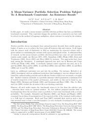
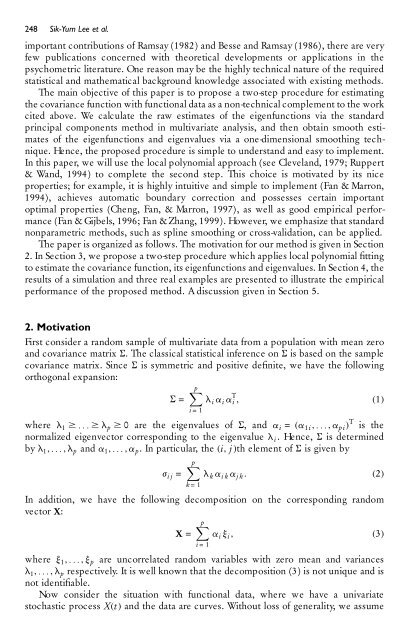
248 Sik-Yum Lee et al.
important contributions of Ramsay (1982) and Besse and Ramsay (1986), there are very
few publications concerned with theoretical developments or applications in the
psychometric literature. One reason may be the highly technical nature of the required
statistical and mathematical background knowledge associated with existing methods.
The main objective of this paper is to propose a two-step procedure for estimating
the covariance function with functional data as a non-technical complement to the work
cited above. We calculate the raw estimates of the eigenfunctions via the standard
principal components method in multivariate analysis, and then obtain smooth estimates
of the eigenfunctions and eigenvalues via a one-dimensional smoothing technique.
Hence, the proposed procedure is simple to understand and easy to implement.
In this paper, we will use the local polynomial approach (see Cleveland, 1979; Ruppert
& Wand, 1994) to complete the second step. This choice is motivated by its nice
properties; for example, it is highly intuitive and simple to implement (Fan & Marron,
1994), achieves automatic boundary correction and possesses certain important
optimal properties (Cheng, Fan, & Marron, 1997), as well as good empirical performance
(Fan & Gijbels, 1996; Fan &Zhang, 1999). However, we emphasize that standard
nonparametric methods, such as spline smoothing or cross-validation, can be applied.
The paper is organized as follows. The motivation for our method is given in Section
2. In Section 3, we propose a two-step procedure which applies local polynomial tting
to estimate the covariance function, its eigenfunctions and eigenvalues. In Section 4, the
results of a simulation and three real examples are presented to illustrate the empirical
performance of the proposed method. A discussion given in Section 5.
2. Motivation
First consider a random sample of multivariate data from a population with mean zero
and covariance matrix S. The classical statistical inference on S is based on the sample
covariance matrix. Since S is symmetric and positive denite, we have the following
orthogonal expansion:
S = Xp
i = 1
l i a i a T i , (1)
where l 1 $ . . . $ l p $ 0 are the eigenvalues of S, and a i = (a 1i , . . . , a pi ) T is the
normalized eigenvector corresponding to the eigenvalue l i . Hence, S is determined
by l 1 , . . . , l p and a 1 , . . . , a p . In particular, the (i, j )th element of S is given by
j i j = Xp
k = 1
l k a i k a j k . (2)
In addition, we have the following decomposition on the corresponding random
vector X:
X = Xp
i = 1
a i y i , (3)
where y 1 , . . . , y p are uncorrelated random variables with zero mean and variances
l 1 , . . . , l p respectively. It is well known that the decomposition (3) is not unique and is
not identiable.
Now consider the situation with functional data, where we have a univariate
stochastic process X(t) and the data are curves. Without loss of generality, we assume