Estimating the covariance function with functional data - Statistics ...
Estimating the covariance function with functional data - Statistics ...
Estimating the covariance function with functional data - Statistics ...
Create successful ePaper yourself
Turn your PDF publications into a flip-book with our unique Google optimized e-Paper software.
247<br />
British Journal of Ma<strong>the</strong>matical and Statistical Psychology (2002), 55, 247–261<br />
© 2002 The British Psychological Society<br />
www.bps.org.uk<br />
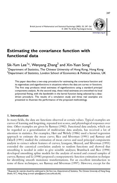
<strong>Estimating</strong> <strong>the</strong> <strong>covariance</strong> <strong>function</strong> <strong>with</strong><br />
<strong>function</strong>al <strong>data</strong><br />
Sik-Yum Lee 1 *, Wenyang Zhang 2 and Xin-Yuan Song 1<br />
1 Department of <strong>Statistics</strong>, The Chinese University of Hong Kong, Hong Kong<br />
2 Department of <strong>Statistics</strong>, London School of Economics & Political Science, UK<br />
This paper describes a two-step procedure for estimating <strong>the</strong> <strong>covariance</strong> <strong>function</strong> and<br />
its eigenvalues and eigen<strong>function</strong>s in situations where <strong>the</strong> <strong>data</strong> are curves or <strong>function</strong>s.<br />
The rst step produces initial estimates of eigen<strong>function</strong>s using a standard principal<br />
components analysis. At <strong>the</strong> second step, <strong>the</strong>se initial estimates are smoo<strong>the</strong>d via local<br />
polynomial tting, <strong>with</strong> <strong>the</strong> bandwidth in <strong>the</strong> kernel <strong>function</strong> being selected by a <strong>data</strong>driven<br />
procedure. The results of a simulation study and three real examples are<br />
presented to illustrate <strong>the</strong> performance of <strong>the</strong> proposed methodology.<br />
1. Introduction<br />
In many elds, <strong>the</strong> <strong>data</strong> are <strong>function</strong>s observed at certain values. Typical examples are<br />
curves of learning and forgetting, repeated test scores, and physiological responses over<br />
time. O<strong>the</strong>r examples are given by Ramsay (1982). Functional <strong>data</strong> analysis, which can<br />
be regarded as a generalization of multivariate <strong>data</strong> analysis, has received a lot of<br />
attention in statistics. For examples, Hart and Wehrly (1986) used a kernel regression<br />
approach to estimate <strong>the</strong> mean curve; Rice and Silverman (1991) and Ramsay and<br />
Dalzell (1991) studied <strong>the</strong> estimation of mean curves and used principal components<br />
analysis to extract salient features of curves; Leurgans, Moyeed, and Silverman (1993)<br />
extended <strong>the</strong> canonical correlation analysis to random <strong>function</strong>s and showed that<br />
smoothing is needed in order to give sensible analyses; Brumback and Rice (1998)<br />
developed smoothing spline models for <strong>the</strong> analysis of nested and crossed samples of<br />
curves; Ramsay and Li (1998) proposed a nonparametric <strong>function</strong> estimation technique<br />
for identifying smooth monotone transformations. For an excellent introduction to<br />
some of <strong>the</strong>se techniques, see Ramsay and Silverman (1997). However, except for <strong>the</strong><br />
* Requests for reprints should be addressed to Sik-Yum Lee, Department of <strong>Statistics</strong>, The Chinese University of Hong Kong,<br />
Shatin, N.T., Hong Kong (e-mail: sylee@sparc2.sta.cuhk.edu.hk).
248 Sik-Yum Lee et al.<br />
important contributions of Ramsay (1982) and Besse and Ramsay (1986), <strong>the</strong>re are very<br />
few publications concerned <strong>with</strong> <strong>the</strong>oretical developments or applications in <strong>the</strong><br />
psychometric literature. One reason may be <strong>the</strong> highly technical nature of <strong>the</strong> required<br />
statistical and ma<strong>the</strong>matical background knowledge associated <strong>with</strong> existing methods.<br />
The main objective of this paper is to propose a two-step procedure for estimating<br />
<strong>the</strong> <strong>covariance</strong> <strong>function</strong> <strong>with</strong> <strong>function</strong>al <strong>data</strong> as a non-technical complement to <strong>the</strong> work<br />
cited above. We calculate <strong>the</strong> raw estimates of <strong>the</strong> eigen<strong>function</strong>s via <strong>the</strong> standard<br />
principal components method in multivariate analysis, and <strong>the</strong>n obtain smooth estimates<br />
of <strong>the</strong> eigen<strong>function</strong>s and eigenvalues via a one-dimensional smoothing technique.<br />
Hence, <strong>the</strong> proposed procedure is simple to understand and easy to implement.<br />
In this paper, we will use <strong>the</strong> local polynomial approach (see Cleveland, 1979; Ruppert<br />
& Wand, 1994) to complete <strong>the</strong> second step. This choice is motivated by its nice<br />
properties; for example, it is highly intuitive and simple to implement (Fan & Marron,<br />
1994), achieves automatic boundary correction and possesses certain important<br />
optimal properties (Cheng, Fan, & Marron, 1997), as well as good empirical performance<br />
(Fan & Gijbels, 1996; Fan &Zhang, 1999). However, we emphasize that standard<br />
nonparametric methods, such as spline smoothing or cross-validation, can be applied.<br />
The paper is organized as follows. The motivation for our method is given in Section<br />
2. In Section 3, we propose a two-step procedure which applies local polynomial tting<br />
to estimate <strong>the</strong> <strong>covariance</strong> <strong>function</strong>, its eigen<strong>function</strong>s and eigenvalues. In Section 4, <strong>the</strong><br />
results of a simulation and three real examples are presented to illustrate <strong>the</strong> empirical<br />
performance of <strong>the</strong> proposed method. A discussion given in Section 5.<br />
2. Motivation<br />
First consider a random sample of multivariate <strong>data</strong> from a population <strong>with</strong> mean zero<br />
and <strong>covariance</strong> matrix S. The classical statistical inference on S is based on <strong>the</strong> sample<br />
<strong>covariance</strong> matrix. Since S is symmetric and positive denite, we have <strong>the</strong> following<br />
orthogonal expansion:<br />
S = Xp<br />
i = 1<br />
l i a i a T i , (1)<br />
where l 1 $ . . . $ l p $ 0 are <strong>the</strong> eigenvalues of S, and a i = (a 1i , . . . , a pi ) T is <strong>the</strong><br />
normalized eigenvector corresponding to <strong>the</strong> eigenvalue l i . Hence, S is determined<br />
by l 1 , . . . , l p and a 1 , . . . , a p . In particular, <strong>the</strong> (i, j )th element of S is given by<br />
j i j = Xp<br />
k = 1<br />
l k a i k a j k . (2)<br />
In addition, we have <strong>the</strong> following decomposition on <strong>the</strong> corresponding random<br />
vector X:<br />
X = Xp<br />
i = 1<br />
a i y i , (3)<br />
where y 1 , . . . , y p are uncorrelated random variables <strong>with</strong> zero mean and variances<br />
l 1 , . . . , l p respectively. It is well known that <strong>the</strong> decomposition (3) is not unique and is<br />
not identiable.<br />
Now consider <strong>the</strong> situation <strong>with</strong> <strong>function</strong>al <strong>data</strong>, where we have a univariate<br />
stochastic process X(t) and <strong>the</strong> <strong>data</strong> are curves. Without loss of generality, we assume
$ $ $<br />
E(X(t)) = 0. Let n(u , v) = Cov(X(u), X(v)) be <strong>the</strong> <strong>covariance</strong> <strong>function</strong>. Viewing <strong>the</strong><br />
random <strong>function</strong> X(t) as a vector <strong>with</strong> innite dimension and tracing <strong>the</strong> idea behind of<br />
(2.1) and (2.2), it is natural to impose <strong>the</strong> following condition on n(u , v): <strong>the</strong>re exists a<br />
series orthonormal <strong>function</strong>s f 1 ( · ), f 2 ( · ), . . . and m 1 m 2 . . . 0, such that <strong>the</strong><br />
<strong>covariance</strong> <strong>function</strong> n(u , v) is given by<br />
n(u , v) = X¥<br />
i = 1<br />
m i f i (u)f i (v), (4)<br />
(see Loeve, 1963). Here <strong>the</strong> m i play <strong>the</strong> role of l i , and <strong>the</strong> f i ( · ) play <strong>the</strong> role of<br />
elements in a i . Moreover, if f i ( · ) and m i , i = 1, 2, . . . , satisfy (4), we have a similar<br />
decomposition on X(t) as in (2.3). More specically,<br />
X(t) = X¥<br />
i = 1<br />
á X, f i ñ f i (t) = X¥<br />
i = 1<br />
h i f i (t), (5)<br />
where á f , gñ = „ f (t)g(t) dt. For i Þ j, and under some regularity conditions, we have<br />
…<br />
…<br />
¼ … …<br />
Eh i h j = E X(t)f i (t) dt X(t)f j (t) dt = EfX(t)X(s)g f i (t)f j (s) dt ds<br />
=<br />
= X¥<br />
… …<br />
n(t, s)f i (t)f j (s) dt ds = X¥<br />
k = 1<br />
k = 1<br />
… …<br />
m k f k (t)f i (t) dt f k (s)f j (s) ds = 0,<br />
m k<br />
… …<br />
f k (t)f k (s)f i (t)f j (s) dt ds<br />
and Eh i = 0, so Cov(h i , h j ) = 0. This implies that h 1 , h 2 , . . . are uncorrelated. Similarly,<br />
for each h i ,<br />
Var(h i ) = X¥ … …<br />
m k f k (t)f i (t) dt f k (s)f i (s) ds = m i .<br />
k = 1<br />
<strong>Estimating</strong> <strong>the</strong> <strong>covariance</strong> <strong>function</strong> <strong>with</strong> <strong>function</strong>al <strong>data</strong> 249<br />
Hence, (5) can be regarded as an extension of (3). Similarly to <strong>the</strong> multivariate case, <strong>the</strong><br />
representations in (4) and (5) are nei<strong>the</strong>r unique nor identiable. If, for any i Þ j,<br />
m i Þ m j , <strong>the</strong>n f i ( · ) is identiable, except for <strong>the</strong> change of sign.<br />
Our development is not hindered by <strong>the</strong> non-identication of (5), because our<br />
interest is in how to estimate n(u , v) and how to nd <strong>the</strong> orthonormal <strong>function</strong>s<br />
f 1 ( · ), f 2 ( · ), . . . that satisfy (4), from <strong>the</strong> observed <strong>function</strong>al <strong>data</strong>. We will call <strong>the</strong>se<br />
orthonormal <strong>function</strong>s f 1 ( · ), f 2 ( · ), . . . <strong>the</strong> eigen<strong>function</strong>s, and <strong>the</strong> corresponding<br />
m 1 , m 2 , . . . <strong>the</strong> eigenvalues of n(u , v).<br />
3. A two-step estimation method<br />
First, let us motivate our method <strong>with</strong> a p-dimensional random vector X. Let ˆl 1 $ . . . $ ˆl p<br />
be <strong>the</strong> eigenvalues of <strong>the</strong> sample <strong>covariance</strong> matrix and â i = (â 1i , . . . , â pi ) T be <strong>the</strong><br />
eigenvector corresponding to ˆl i . An estimate of <strong>the</strong> (i, j )th element of S is given by<br />
ĵ i j = Xp<br />
k = 1<br />
ˆl k â i k â j k .<br />
The idea will be used to handle <strong>function</strong>al <strong>data</strong> as follows.
250 Sik-Yum Lee et al.<br />
Now suppose we have a univariate stochastic process X(t); <strong>with</strong>out loss of<br />
generality, we assume E(X(t)) = 0 and t [ [0, 1]. Let X 1 ( · ), . . . , X m ( · ) be a collection<br />
of m sample curves, each observed at t 1 , . . . , t n . More explicitly, we have <strong>the</strong> <strong>data</strong> set<br />
X h (t i ), i = 1, . . . , n, h = 1, . . . , m. For simplicity, we denote X h (t i ) by X i h . Obviously, for<br />
i, k = 1, . . . , n, and h, l = 1, . . . , m, we have EX i h = 0 and<br />
<br />
0, h Þ l,<br />
Cov(X i h , X kl ) =<br />
n(t i , t k ), h = l.<br />
Our procedure in estimating n(u, v), m i and f i ( · ) involves <strong>the</strong> following two steps.<br />
Step 1. Ignore temporarily <strong>the</strong> fact that <strong>the</strong> <strong>data</strong> are continuous <strong>function</strong>s and treat<br />
<strong>the</strong> problem as a standard principal components problem in multivariate analysis.<br />
Specically, let S be <strong>the</strong> sample <strong>covariance</strong> matrix <strong>with</strong> (i, j )th element<br />
1<br />
m<br />
X m<br />
k = 1<br />
X i k X j k .<br />
Compute n ˆm 1 $ . . . $ n ˆm n , <strong>the</strong> eigenvalues of S; and n ± 1/2 ˆûj = (n ± 1/2 ˆb1 j , . . . , n ± 1/2 ˆbn j ) T ,<br />
<strong>the</strong> orthonormal eigenvector corresponding to <strong>the</strong> eigenvalue n ˆm j , for j = 1, . . . , n.<br />
Step 2. For each j, we treat ( ˆb 1 j , t 1 ), . . . , ( ˆb n j , t n ) as a sample of size n from <strong>the</strong><br />
regression model<br />
Y = f j (t) + « , (6)<br />
where Y is <strong>the</strong> ˆb. For each j = 1, . . . , n , smooth ˆb 1 j , . . . , ˆb n j <strong>with</strong> respect to t 1 , . . . , t n , and<br />
obtain an estimate of <strong>the</strong> eigen<strong>function</strong>, ˆf j ( · ).<br />
The procedure for estimating <strong>the</strong> eigenvalue m j of <strong>the</strong> <strong>covariance</strong> <strong>function</strong> n( · , · ) is<br />
as follows. For j = 1, 2, . . . , n, <strong>the</strong> j th eigenvalue of <strong>the</strong> <strong>covariance</strong> <strong>function</strong> of X(t) is <strong>the</strong><br />
variance of<br />
h j =<br />
…<br />
X(t)f j (t) dt <<br />
and f j (t i ) can be estimated by ˆf j (t i ). Hence,<br />
Fur<strong>the</strong>rmore, let<br />
˜h kj = 1 n<br />
h j <<br />
X n<br />
i = 1<br />
The sample variance of ˜h j is given by<br />
dVar(h j ) = 1 m<br />
˜h j = 1 n<br />
X n<br />
i = 1<br />
1<br />
n<br />
X n<br />
i = 1<br />
X(t i ) ˆf j (t i ).<br />
X(t i )f j (t i )<br />
X ki ˆfj (t i ), k = 1, . . . , m.<br />
X Á m<br />
˜h k j ± 1 X ! m 2 ˜h k j<br />
m<br />
.<br />
k = 1<br />
k = 1<br />
This gives an estimate for <strong>the</strong> variance of h j and hence <strong>the</strong> j th eigenvalue m j of <strong>the</strong><br />
<strong>covariance</strong> <strong>function</strong> n(u, v). Finally, an estimate of n(u , v) is given by<br />
ˆn(u , v) = Xn<br />
j = 1<br />
ˆm j ˆfj (u) ˆf j (v). (7)<br />
The initial estimator ˆû j is a rough estimator for f j ( · ). In <strong>the</strong> second step, a much<br />
better estimator, ˆfj ( · ), is obtained via an application of a smoothing technique to
( ˆb 1 j , t 1 ), . . . , ( ˆb n j , t n ). By this smoothing step, information from neighbouring points is<br />
pooled toge<strong>the</strong>r to improve <strong>the</strong> efciency of <strong>the</strong> raw initial estimator. Many standard<br />
nonparametric methods, such as wavelet thresholding (Donoho, 1995; Donoho &<br />
Johnstone, 1995), spline smoothing (Eubank, 1988; Wahba, 1990; Green and Silverman,<br />
1994), or local polynomial modelling (Cleveland, 1979; Ruppert and Wand, 1994) can<br />
be used to nd ˆf j ( · ) in <strong>the</strong> second step. Therefore, <strong>the</strong> proposed two-step procedure is<br />
conceptually very simple; it just involves <strong>the</strong> computation of eigenvalues and eigenvectors<br />
of a sample <strong>covariance</strong> matrix using standard principal components analysis,<br />
and <strong>the</strong>n a standard one-dimensional nonparametric smoothing. Implementation of<br />
this procedure is quite straightforward.<br />
A nonparametric method in estimating eigenvalues/eigen<strong>function</strong>s of a <strong>covariance</strong><br />
structure <strong>with</strong> curve <strong>data</strong> has been developed by Rice and Silverman (1991). In <strong>the</strong>ir<br />
method, a class of estimates was obtained by bounding <strong>the</strong> roughness of <strong>the</strong> eigen<strong>function</strong><br />
via maximizing u T Su subject to k u k = 1 and u T Du # g, where g is a smoothing<br />
parameter and D is a roughening matrix, say F T F <strong>with</strong> a second-differencing operator F.<br />
The smoothing parameter g was selected by cross-validation based on a prediction<br />
viewpoint. After obtaining <strong>the</strong> rst j eigen<strong>function</strong>s, <strong>the</strong> ( j + 1)th eigen<strong>function</strong> was<br />
obtained by repeating <strong>the</strong> procedure of obtaining <strong>the</strong> eigen<strong>function</strong> in <strong>the</strong> orthogonal<br />
complement of <strong>the</strong> space generated by <strong>the</strong> rst j eigen<strong>function</strong>s. This process was<br />
continued until all n eigen<strong>function</strong>s were obtained. Evaluation of g via cross-validation is<br />
required to obtain each of <strong>the</strong> eigen<strong>function</strong>s. Hence, this method is not two-step in<br />
nature and is quite different from our simple two-step procedure.<br />
Motivated by many of its nice properties, we use <strong>the</strong> local polynomial approach to<br />
compute ˆf j ( · ) in <strong>the</strong> second step of our procedure. It has been shown that odd-order<br />
polynomial ts are preferable to even order polynomial ts (Fan & Gijbels, 1996), so we<br />
use a local polynomial of odd order q to estimate <strong>the</strong> underlying <strong>function</strong>. For each point<br />
t 0 , we approximate <strong>the</strong> underlying <strong>function</strong> f j (t) locally by<br />
f j (t) <<br />
X q<br />
1<br />
k! f(k) j<br />
k = 0<br />
(t 0 )(t ± t 0 ) k = Xq<br />
k = 0<br />
, k (t ± t 0 ) k , (8)<br />
for t in a neighbourhood of t 0 . This leads to <strong>the</strong> following local least squares problem:<br />
minimize<br />
( )<br />
X n<br />
2<br />
ˆb i j ± Xq<br />
, k (t i ± t 0 ) k K h j<br />
(t i ± t 0 ), (9)<br />
i = 1<br />
k = 0<br />
<strong>Estimating</strong> <strong>the</strong> <strong>covariance</strong> <strong>function</strong> <strong>with</strong> <strong>function</strong>al <strong>data</strong> 251<br />
<strong>with</strong> respect to , k , k = 0, . . . , q, for a given kernel <strong>function</strong> K and a bandwidth h j ,<br />
where K h ( · ) = K( · /h)/h. Let W(h) = diag(K h (t 1 ± t 0 ), . . . , K h (t n ± t 0 )), and<br />
0<br />
1 (t 1 ± t 0 ) . . . (t 1 ± t 0 ) q 1<br />
T q =<br />
. . .<br />
. . .<br />
.<br />
B<br />
C<br />
@<br />
. . A .<br />
1 (t n ± t 0 ) . . . (t n ± t 0 ) q<br />
The solution of <strong>the</strong> least squares problem (9) gives <strong>the</strong> following estimate of <strong>the</strong><br />
underlying <strong>function</strong> at t 0 . More specically, <strong>the</strong> estimate ˆf j (t 0 ) is equal to <strong>the</strong> rst<br />
element of <strong>the</strong> matrix:<br />
(T T q W(h j )T q ) ± 1 T T q W(h j ) ˆû j . (10)<br />
Since ˆû j , j = 1, . . . , n are orthonormal, after this local polynomial smoothing, ˆfj ( · ),<br />
j = 1, . . . , n are approximately orthonormal.
252 Sik-Yum Lee et al.<br />
In <strong>the</strong> smoothing procedure, <strong>the</strong> bandwidth h j plays an important role. In general, a<br />
bandwidth h j = 0 basically results in interpolating <strong>the</strong> <strong>data</strong>, and hence leads to <strong>the</strong> most<br />
complex model. A bandwidth h j = ¥ corresponds to tting globally a polynomial of<br />
degree q, and hence leads to <strong>the</strong> simplest model. Although we use a <strong>data</strong>-driven method<br />
(see Fan and Gijbels, 1995; Zhang and Lee, 2000) to select <strong>the</strong> bandwidth in this paper,<br />
<strong>the</strong>re are o<strong>the</strong>r procedures, such as cross-validation, which can be implemented by<br />
S-PLUS (see Venables and Ripley, 1999).<br />
As pointed out by Castro, Lawton, and Sylvestre (1986), if <strong>the</strong> prime points t i are not<br />
equally spaced, <strong>the</strong> following adjustment is required in <strong>the</strong> rst step of <strong>the</strong> two-step<br />
procedure to ensure <strong>the</strong> invariance of eigen<strong>function</strong>s <strong>with</strong> respect to different choices<br />
of design. Using <strong>the</strong> quadrature rule (see Baker, 1977), we obtain<br />
w i =<br />
… 1<br />
0<br />
l i (t) dt, where l i (t) =<br />
Y n<br />
j = 0, j Þ<br />
i<br />
t ± t j<br />
t i ± t j<br />
. (11)<br />
Let A = diag(w 1 , . . . , w n ), and ˆm i <strong>the</strong> i th eigenvalue of A 1/2 SA 1/2 . Let ˜û i be <strong>the</strong> i th<br />
orthonormal eigenvector of A 1/2 SA 1/2 corresponding to eigenvalue ˆm i . The initial rststep<br />
estimates are obtained via ˆû i = A ± 1/2 ˜ûi , i = 1, . . . , n. These estimates are <strong>the</strong>n<br />
smoo<strong>the</strong>d at <strong>the</strong> second step for obtaining <strong>the</strong> nal estimates of <strong>the</strong> eigen<strong>function</strong>s. For<br />
unequally spaced sampling all inner products must use <strong>the</strong> quadrature rule, so when we<br />
estimate <strong>the</strong> j th eigenvalue m j of <strong>the</strong> <strong>covariance</strong> <strong>function</strong> n(u , v), ˜h k j becomes<br />
˜h k j = Xn<br />
i = 1<br />
X ki ˆfj (t i )w i .<br />
The modication of <strong>the</strong> proposed two-step procedure for dealing <strong>with</strong> <strong>the</strong> unequally<br />
spaced case is minor. In <strong>the</strong> rst step, after obtaining <strong>the</strong> diagonal matrix A that contains<br />
<strong>the</strong> weights w i , we obtain <strong>the</strong> eigenvalues and orthonormal eigenvectors of A 1/2 SA 1/2<br />
and <strong>the</strong> initial rst-step estimate of <strong>the</strong> eigen<strong>function</strong> ˆb i , i = 1, . . . , n. At <strong>the</strong> second step<br />
for producing <strong>the</strong> nal estimates, <strong>the</strong> standard one-dimensional nonparametric smoothing<br />
is conducted on <strong>the</strong> basis of <strong>the</strong> regression model (6), <strong>with</strong> <strong>the</strong> sample<br />
( ˆb 1 j , t 1 ), . . . , ( ˆb n j , t n ) for each j. Again, this step can be completed by using a local<br />
polynomial <strong>data</strong>-driven method or by software packages such as SAS and S-PLUS.<br />
4. Numerical illustrations<br />
4.1. A simulation study<br />
The following example is used to illustrate <strong>the</strong> performance of our method for<br />
estimating <strong>covariance</strong> <strong>function</strong>s, <strong>the</strong>ir eigen<strong>function</strong>s and eigenvalues. Consider<br />
X(t) =<br />
p <br />
2 sin(pt)y1 +<br />
p <br />
2 cos(pt)y2 , t [ [0, 1].<br />
Random variables y 1 and y 2 in this example are independently and normally distributed<br />
<strong>with</strong> mean zero. Their variances are equal to f2.0, 1.0g. The numbers of sample points<br />
for each sample curve were selected to be n = 15, 50, 100 and 200; and for each n we<br />
took m = 50, 100, and 200. Sample points of <strong>the</strong> sample curve were observed at (i)<br />
equally spaced points t i = i/(n + 1), i = 1, . . . , n; and (ii) unequally spaced points<br />
obtained from sorted random points simulated from a uniform distribution on [0, 1].<br />
For cases (i) and (ii) <strong>with</strong> different n and m, <strong>the</strong> number of replications was 200.
pThe truep <strong>covariance</strong>p <strong>function</strong> pof X(t) in this example is: n(u, v) =<br />
2p2<br />
sin(pu) p 2 sin(pv) + 2 cos(pu) 2 cos(pv). The eigen<strong>function</strong>s are equal to<br />
f 2 sin(pt), 2 cos(pt)g. Note that <strong>the</strong>se eigen<strong>function</strong>s are not unique; <strong>the</strong>y allow<br />
sign differences. The mean integrated square error (MISE)<br />
… …<br />
D ± 1 E (ˆn(u , v) ± n(u , v)) 2 du dv,<br />
where <strong>the</strong> D is <strong>the</strong> support set of (u, v), is employed as <strong>the</strong> criterion to evaluate <strong>the</strong><br />
performance of <strong>the</strong> estimator.<br />
The proposed procedure was used to estimate <strong>the</strong> <strong>covariance</strong> <strong>function</strong>s and nd<br />
<strong>the</strong>ir eigen<strong>function</strong>s and eigenvalues. Local linear t (q = 1) and local cubic t (q = 3)<br />
for <strong>the</strong> regression curve are considered, and <strong>the</strong> kernel <strong>function</strong> is taken to be <strong>the</strong><br />
Epanechnikov kernel K(t) = 0.75(1 ± t 2 ) + . The MISEs of <strong>the</strong> estimators are reported in<br />
Table 1. The following phenomena are observed from this table: (i) Generally, <strong>the</strong> MISE<br />
improved signicantly <strong>with</strong> increase of sample size m. (ii) The MISE <strong>with</strong> n = 50 has a<br />
signicant improvement over <strong>the</strong> case <strong>with</strong> n = 15. However, changes in MISE are very<br />
small for situations <strong>with</strong> n larger than 50. Most probably, <strong>the</strong> reason for this phenomenon<br />
is that, <strong>with</strong> a signicantly large number of points, <strong>the</strong> information between<br />
adjacent points does not contribute in improving <strong>the</strong> accuracy of <strong>the</strong> estimator.<br />
Differences between linear t and cubic t are very small for large n. (iii) To achieve<br />
more accurate results, it is more important to have a large m than large n. (iv) The<br />
differences in MISE between <strong>the</strong> equally and unequally spaced cases are not substantial,<br />
especially <strong>with</strong> moderate sample sizes. Roughly speaking, performance of a cubic t for<br />
n = 15 and m = 50 is acceptable.<br />
Table 1. Mean integrated square errors in simulation study<br />
<strong>Estimating</strong> <strong>the</strong> <strong>covariance</strong> <strong>function</strong> <strong>with</strong> <strong>function</strong>al <strong>data</strong> 253<br />
n<br />
m q 15 50 100 200<br />
Equally 50 1 0.316 0.274 0.275 0.275<br />
spaced 3 0.288 0.279 0.277 0.275<br />
100 1 0.198 0.137 0.137 0.137<br />
3 0.145 0.139 0.138 0.138<br />
200 1 0.130 0.063 0.063 0.062<br />
3 0.066 0.063 0.063 0.063<br />
Unequally 50 1 0.344 0.303 0.275 0.266<br />
spaced 3 0.325 0.305 0.277 0.266<br />
100 1 0.214 0.160 0.140 0.132<br />
3 0.178 0.159 0.141 0.132<br />
200 1 0.139 0.083 0.066 0.061<br />
3 0.093 0.080 0.066 0.061<br />
From <strong>the</strong> 200 replications, we select <strong>the</strong> estimator <strong>with</strong> <strong>the</strong> median performance for<br />
a fur<strong>the</strong>r illustration of <strong>the</strong> performance of <strong>the</strong> procedure. Since results produced by<br />
cubic t are similar, only results obtained from <strong>the</strong> linear t are presented. Estimates of<br />
eigenvalues <strong>with</strong> linear t for some choices of n and m are presented in Table 2. As<br />
expected, under <strong>the</strong> same m, results for different large n are similar, so are not
254 Sik-Yum Lee et al.<br />
presented. It seems that <strong>the</strong> eigenvalue estimates are reasonably accurate. Figure 1<br />
depicts <strong>the</strong> resulting estimated eigen<strong>function</strong>s <strong>with</strong> n = 200 and m = 200 for equally<br />
spaced and unequally spaced cases. It can be seen that <strong>the</strong> true and <strong>the</strong> estimated<br />
eigen<strong>function</strong>s are close to each o<strong>the</strong>r. To study empirically whe<strong>the</strong>r <strong>the</strong> orthogonality<br />
among <strong>the</strong> original components is affected by separate smoothing, we compute<br />
( ˆf j , ˆf j ¢ ) = Xn<br />
i = 1<br />
ˆf j (t i ) ˆf j ¢ (t i )<br />
for all pairs of ˆf j and ˆf j ¢ . For <strong>the</strong> equally spaced case, ( ˆf 1 , ˆf 2 ) for (n, m) = (15, 50),<br />
(50, 50), (100, 100), and (200, 200) are equal to ± 3.65 ´ 10 ± 4 , ± 1.88 ´ 10 ± 6 ,<br />
1.18 ´ 10 ± 7 and 1.69 ´ 10 ± 8 , respectively. It seems that for moderate sizes n and<br />
m, orthogonality is not seriously affected by separate smoothing of <strong>the</strong> different<br />
components. A similar phenomenon is also observed for <strong>the</strong> unequally spaced case.<br />
Table 2. Estimates of eigenvalues in simulation study<br />
(n, m)<br />
True<br />
value (15, 50) (50, 50) (100, 100) (200, 200)<br />
Equally 2.0 2.17 2.42 1.89 2.20<br />
spaced 1.0 1.47 0.73 0.98 1.05<br />
Unequally 2.0 3.05 1.77 2.07 2.12<br />
spaced 1.0 0.81 0.81 0.89 1.09<br />
4.2. Real examples<br />
We rst illustrate our method by an application to <strong>the</strong> tongue <strong>data</strong> given in Besse and<br />
Ramsay (1986, pp. 288–289). The <strong>data</strong> consist of 42 records of tongue dorsum movements<br />
collected by Munhall (1984) using an ultrasound sensing technique developed by<br />
Keller and Ostry (1983). It will be assumed that <strong>the</strong> interval of <strong>the</strong> observation has been<br />
normalized to be [0, p], and <strong>the</strong> sampled values are observations at 13 equally spaced<br />
points. See Besse and Ramsay (1986) for more detailed background on this <strong>data</strong> set. The<br />
proposed two-step procedure <strong>with</strong> a cubic t at <strong>the</strong> second step is used to nd <strong>the</strong><br />
eigen<strong>function</strong>s and <strong>the</strong>ir eigenvalues of <strong>the</strong> <strong>covariance</strong> <strong>function</strong>s.<br />
Figure 2 describes <strong>the</strong> rst three eigen<strong>function</strong>s of <strong>the</strong> sample <strong>function</strong>s. Using<br />
…<br />
Var(X(t)) dt<br />
to measure <strong>the</strong> variation of <strong>the</strong> random <strong>function</strong> X(t), we nd that <strong>the</strong> rst three<br />
eigen<strong>function</strong>s account for 89.5%, 8.4%and 1.4%of <strong>the</strong> overall variation of <strong>the</strong> sample<br />
<strong>function</strong>s, respectively. These three eigen<strong>function</strong>s account for a total of 99.3%of <strong>the</strong><br />
overall variance. It can be seen from Fig. 2 that <strong>the</strong> rst eigen<strong>function</strong> can be regarded as<br />
constant (compared <strong>with</strong> o<strong>the</strong>r eigen<strong>function</strong>s), <strong>the</strong> second is close to sin(t), and <strong>the</strong><br />
third is close to cos(t). Our results are very similar to those obtained by Besse and<br />
Ramsay (1986), in which <strong>the</strong> eigenvalues respectively account for 90.0%, 8.3%and 1.5%<br />
of <strong>the</strong> variation, and <strong>the</strong> eigen<strong>function</strong>s are also very similar (see Besse & Ramsay, 1986,<br />
Fig. 5). At a reviewer’s suggestion, <strong>the</strong> estimated <strong>covariance</strong> <strong>function</strong> is shown in Fig. 3.
<strong>Estimating</strong> <strong>the</strong> <strong>covariance</strong> <strong>function</strong> <strong>with</strong> <strong>function</strong>al <strong>data</strong> 255<br />
Figure 1. Estimated<br />
p <br />
eigen<strong>function</strong>s<br />
p <br />
for (a) <strong>the</strong> equally and (b) <strong>the</strong> unequally spaced cases. The solid<br />
curves are (i) 2 sin(pt), (ii) ± 2 cos(pt).<br />
Hence <strong>the</strong> analysis via <strong>the</strong> proposed two-step procedure also suggests <strong>the</strong> following<br />
model as in Besse and Ramsay (1986):<br />
X(t) = y 1 + y 2 sin(t) + y 3 cos(t) + e(t),<br />
and leads to <strong>the</strong> similar conclusion that <strong>the</strong> simple harmonic motion describes tongue<br />
dorsum behaviour adequately in [0, p].<br />
As a second illustrative example, we reanalyse <strong>the</strong> curves of saggital hip angles in<br />
Rice and Silverman (1991). In this <strong>data</strong> set, n = 20 and m = 39, and observations are<br />
taken over a gait cycle consisting of one (double) step taken by each child; see Olshen,<br />
Biden, Wyatt, and Su<strong>the</strong>rland (1989) for more details. Using <strong>the</strong> proposed two-step<br />
procedure <strong>with</strong> a cubic t at <strong>the</strong> second step, we obtained <strong>the</strong> rst four eigen<strong>function</strong>s.<br />
The corresponding eigenvalues respectively account for 70.6%, 12.1%, 8.4%and 3.8%(a<br />
total of 94.9%) of <strong>the</strong> total variability. These results are very close to those reported in<br />
Rice and Silverman (1991). The eigen<strong>function</strong>s are depicted in Fig. 4. Comprising this<br />
gure <strong>with</strong> Fig. 2 in Rice and Silverman (1991), it is clear that eigen<strong>function</strong>s obtained<br />
from our procedure and <strong>the</strong>ir procedures are also similar. The fourth eigen<strong>function</strong> is<br />
not very close to <strong>the</strong> raw eigenvector, which may indicate that <strong>the</strong> amount of noise of<br />
<strong>the</strong> raw eigenvector ltered by <strong>the</strong> local polynomial smoothing is substantial. In any
256 Sik-Yum Lee et al.<br />
Figure 2. The rst three eigen<strong>function</strong>s of <strong>the</strong> tongue <strong>data</strong>; <strong>the</strong> rst, second and third eigen<strong>function</strong>s<br />
are represented by <strong>the</strong> solid, dotted and dashed curves, respectively.<br />
Figure 3. Covariance <strong>function</strong> of <strong>the</strong> tongue <strong>data</strong>. The height of <strong>the</strong> surface indicates <strong>the</strong> amount of<br />
<strong>covariance</strong>.
<strong>Estimating</strong> <strong>the</strong> <strong>covariance</strong> <strong>function</strong> <strong>with</strong> <strong>function</strong>al <strong>data</strong> 257<br />
Figure 4. First four raw eigenvectors (dots) and smoo<strong>the</strong>d eigen<strong>function</strong> (solid curve) of <strong>the</strong> hip angle<br />
<strong>data</strong>.<br />
case, since it is <strong>the</strong> least important eigen<strong>function</strong>, statistical conclusions drawn on <strong>the</strong><br />
basis of <strong>the</strong> analysis are not affected. For completeness, <strong>the</strong> estimated <strong>covariance</strong><br />
<strong>function</strong> is displayed in Fig. 5. Detailed interpretations of <strong>the</strong> results, which are available<br />
in Rice and Silverman (1991), are not presented to save space.<br />
Our nal example is based on a variable selected from a study (Mackinnon et al.,<br />
1991) of school smoking-prevention programmes based on social-psychological principles.<br />
These social inuence programmes were designed to teach social skills and to<br />
create a social environment less receptive to drug use. If <strong>the</strong>y work as planned, <strong>the</strong>n<br />
favourable changes in mediating variables for drug use and behavioural intentions are<br />
indicators of success. One of <strong>the</strong> main objectives of <strong>the</strong> study was to evaluate <strong>the</strong> impact<br />
of a social inuence based programme on <strong>the</strong> mediating variables it was designed to<br />
change. The <strong>data</strong> were obtained from public middle schools and junior high schools in<br />
midwestern states of USA. As an illustration, we considered a variable X(t) measuring<br />
students’ control of <strong>the</strong>ir cigarette consumption (<strong>the</strong> original question is: ‘If your best<br />
friend offered you a cigarette, how hard would it be to refuse <strong>the</strong> offer?’), measured at<br />
ve time points for students from 50 schools. At t = t 0 , all students were in <strong>the</strong> seventh<br />
grade; t 1 was six months later and <strong>the</strong> o<strong>the</strong>r time intervals were one year. Hence, <strong>the</strong>
258 Sik-Yum Lee et al.<br />
Figure 5. Covariance <strong>function</strong> of <strong>the</strong> hip <strong>data</strong>. The height of <strong>the</strong> surface indicates <strong>the</strong> amount of<br />
<strong>covariance</strong>.<br />
time points are not equally spaced. Using <strong>the</strong> proposed procedure <strong>with</strong> an adjustment<br />
for unequally spaced time points, we found that <strong>the</strong> rst two eigenvalues respectively<br />
accounted for 68.3%and 17.0%of <strong>the</strong> total variability. The corresponding eigen<strong>function</strong>s<br />
obtained via a local polynomial smoothing <strong>with</strong> a linear t are displayed in Fig. 6.<br />
Roughly, <strong>the</strong>se eigen<strong>function</strong>s can be regarded as quadratic. They reveal <strong>the</strong> change in<br />
students’ control of cigarette consumption over time. From <strong>the</strong> rst eigen<strong>function</strong>, it<br />
seems that <strong>the</strong> time that students’ best friend has <strong>the</strong> strongest inuence is between half<br />
and one year after seventh grade, after which <strong>the</strong> best friend’s inuence decreases.<br />
However, it should be pointed out that this is just an illustrative example <strong>with</strong> only ve<br />
time points, and its interpretation should be treated <strong>with</strong> caution. More <strong>data</strong> on more<br />
time points are required for a more substantive conclusion to be drawn.<br />
Several examples given in Ramsay and Silverman (1997) have been analysed. We<br />
observe that results obtained via <strong>the</strong> proposed two-step procedure are similar to those<br />
reported in Ramsay and Silverman (1997).<br />
5. Discussion<br />
Functional <strong>data</strong> analysis is particularly useful for investigating changes over time for<br />
characteristics that are measured continuously or repeatedly for each object. Examples<br />
of this type of research are longitudinal studies, and analyses of growth curves and<br />
learning curves. It is not straightforward to extend <strong>the</strong> classical multivariate <strong>data</strong> analysis<br />
to <strong>function</strong>al <strong>data</strong> analysis. As a complement to <strong>the</strong> existing work, this paper proposes a<br />
simple two-step procedure to estimate <strong>the</strong> <strong>covariance</strong> <strong>function</strong> and its eigenvalues and
<strong>Estimating</strong> <strong>the</strong> <strong>covariance</strong> <strong>function</strong> <strong>with</strong> <strong>function</strong>al <strong>data</strong> 259<br />
Figure 6. The rst two eigen<strong>function</strong>s of <strong>the</strong> <strong>data</strong> on school smoking-prevention programme; <strong>the</strong> rst<br />
and second <strong>function</strong>s are represented by <strong>the</strong> solid and dotted curves, respectively.<br />
eigen<strong>function</strong>s. At <strong>the</strong> rst step, we compute <strong>the</strong> eigenvectors and eigenvalues of<br />
certain sample <strong>covariance</strong> matrices. This task can be completed easily and efciently<br />
using standard software. The second step only involves some one-dimensional nonparametric<br />
smoothing, simpler than <strong>the</strong> multi-dimensional smoothing required by o<strong>the</strong>r<br />
methods. Our simulation results indicate that <strong>the</strong> results produced are quite accurate.<br />
The proposed procedure also gives very similar results to those in Besse and Ramsay<br />
(1986) and Rice and Silverman (1991) in analysing some real examples. Hence, it is<br />
simple to understand, easy to implement, and efcient in producing reliable results.<br />
Owing to <strong>the</strong> optimal statistical properties associated <strong>with</strong> <strong>the</strong> local polynomial<br />
smoothing, we apply it to obtain <strong>the</strong> nal eigen<strong>function</strong>s at <strong>the</strong> second step of <strong>the</strong><br />
proposed procedure. In fact, o<strong>the</strong>r methods such as spline smoothing can be used. The<br />
available code for most of <strong>the</strong>se more traditional methods can be found in existing<br />
software such as SAS, S-PLUS and Matlab. For practitioners, <strong>the</strong> smoothing at <strong>the</strong> second<br />
step can be completed via <strong>the</strong> above standard software. Hence, <strong>the</strong> proposed procedure<br />
can be used by those <strong>with</strong> less technical training. Owing to <strong>the</strong> pioneering work of<br />
Ramsay and Dalzell (1991), Ramsay and Silverman (1997) and o<strong>the</strong>rs, we expect that<br />
<strong>function</strong>al <strong>data</strong> analysis will gain in popularity, and that <strong>the</strong> standard software will<br />
include an option to perform local polynomial smoothing in <strong>the</strong> near future.<br />
Acknowledgements<br />
The research for this paper was partiallysupported by a grant from <strong>the</strong> Research Grants Council of<br />
<strong>the</strong> Hong Kong Special Administration Region, China (Project No. CVHK 4346/OIH), and a direct
260 Sik-Yum Lee et al.<br />
grant from CVHK. The authors are greatly indebted to <strong>the</strong> Editor and two reviewers for some<br />
valuable comments for improvement of <strong>the</strong> paper, and thankful to Drs M. A. Pentz and C. P. Chou<br />
for providing <strong>the</strong> <strong>data</strong> in <strong>the</strong> last real example. The assistance of Es<strong>the</strong>r L. S. Tam in preparing <strong>the</strong><br />
manuscript is also acknowledged.<br />
References<br />
Baker, C. T. H. (1977). The numerical treatment of integral equations. Oxford: Clarendon Press.<br />
Besse, P., & Ramsay, J. O. (1986). Principal components analysis of sampled <strong>function</strong>s.<br />
Psychometrika, 51, 285–311.<br />
Brumback, B. A., & Rice, J. A. (1998). Smoothing spline models for <strong>the</strong> analysis of nested and<br />
crossed samples of curves (<strong>with</strong> discussion). Journal of <strong>the</strong> American Statistical Association,<br />
93, 961–994.<br />
Castro, P. E., Lawton, W. H., & Sylvestre, E. A. (1986). Principal modes of variation for process <strong>with</strong><br />
continuous sample curves. Technometrics, 28, 329–337.<br />
Cheng, M. Y., Fan, J., & Marron, J. S. (1997). On automatic boundary corrections. Annals of<br />
<strong>Statistics</strong>, 25, 1691–1708.<br />
Cleveland, W. S. (1979). Robust locally weighted regression and smoothing scatterplots. Journal<br />
of <strong>the</strong> American Statistical Association, 74, 829 –836.<br />
Donoho, D. L. (1995). Nonlinear solution of linear inverse problems by wavelet-vaguelette<br />
decomposition. Applied and Computational Harmonic Analysis, 2, 101–126.<br />
Donoho, D. L., & Johnstone, I. M. (1995). Adapting to unknown smoothness via wavelet<br />
shrinkage. Journal of <strong>the</strong> American Statistical Association, 90, 1200–1224.<br />
Eubank, R. L. (1988). Spline smoothing and nonparametric regression. New York: Marcel Dekker.<br />
Fan, J., & Gijbels, I. (1995). Data-driven bandwidth selection in local polynomial tting: variable<br />
bandwidth and spatial adaptation. Journal of <strong>the</strong> Royal Statistical Society, Series B, 57,<br />
371 –394.<br />
Fan, J., & Gijbels, I. (1996). Local polynomial modelling and its applications. London: Chapman<br />
& Hall.<br />
Fan, J., & Marron, J. S. (1994). Fast implementation of nonparametric curve estimator. Journal of<br />
Computational and Graphical <strong>Statistics</strong>, 3, 35–56.<br />
Fan, J., & Zhang, W. (1999). Statistical estimation in varying coefcient models. Annals of<br />
<strong>Statistics</strong>, 27, 1491–1518.<br />
Green, P. J., &Silverman, B. W. (1994). Nonparametric regression and generalized linear models:<br />
A roughness penalty approach. London: Chapman & Hall.<br />
Hart, J. D., &Wehrly, T. E. (1986). Kernel regression estimation using repeated measurements <strong>data</strong>.<br />
Journal of <strong>the</strong> American Statistical Association, 81, 1080–1088.<br />
Keller, E., & Ostry, D. J. (1983). Computerized measurement of tongue dorsum movements <strong>with</strong><br />
pulsed-echo ultrasound. Journal of <strong>the</strong> Acoustical Society of America, 73, 1309–1315.<br />
Leurgans, S. E., Moyeed, R. A., & Silverman, B. W. (1993). Canonical correlation analysis when <strong>the</strong><br />
<strong>data</strong> are curves. Journal of <strong>the</strong> Royal Statistical Society, Series B, 55, 725–740.<br />
Loeve, M. (1963). Probability <strong>the</strong>ory, 3rd ed. Princeton, N.J.: D. Van Nostrand.<br />
Mackinnon, D. P., Johnson, C. A., Pentz, M. A., Dwyer, J. H., Hansen, W. B., Flay, B. R., & Wang,<br />
E. Y.-I. (1991). Mediating mechanism in a school-based drug prevention program: First year<br />
effects of <strong>the</strong> midwestern prevention project. Health Psychology, 10, 164–172.<br />
Munhall, K. G. (1984). Temporal adjustment in speech motor control: Evidence from laryngeal<br />
kinematics. Unpublished doctoral dissertation, McGill University.<br />
Olshen, R. A., Biden, E. N., Wyatt, M. P., &Su<strong>the</strong>rland, D. H. (1989). Gait analysis and <strong>the</strong> bootstrap.<br />
Annals of <strong>Statistics</strong>, 17, 1419–1440.<br />
Ramsay, J. O. (1982). When <strong>the</strong> <strong>data</strong> are <strong>function</strong>s. Psychometrika , 47, 379–396.<br />
Ramsay, J. O., & Dalzell, C. J. (1991). Some tools for <strong>function</strong>al <strong>data</strong> analysis (<strong>with</strong> discussions).<br />
Journal of <strong>the</strong> Royal Statistical Society, Series B, 53, 539–572.
Ramsay, J. O., & Silverman, B. W. (1997). Functional <strong>data</strong> analysis. New York: Springer-Verlag.<br />
Ramsay, J. O., & Li, X. (1998). Curve registration. Journal of <strong>the</strong> Royal Statistical Society, Series B,<br />
60, 351–363.<br />
Rice, J. A., & Silverman, B. W. (1991). <strong>Estimating</strong> <strong>the</strong> mean and <strong>covariance</strong> structure nonparametrically<br />
when <strong>the</strong> <strong>data</strong> are curves. Journal of <strong>the</strong> Royal Statistical Society, Series B,<br />
53, 233–243.<br />
Ruppert, D., & Wand, M. P. (1994). Multivariate weighted least squares regression. Annals of<br />
<strong>Statistics</strong>, 22, 1346–1370.<br />
Venables, W. N., & Ripley, B. D. (1999). Modern applied statistics <strong>with</strong> S-PLUS, 3rd ed. New York:<br />
Springer-Verlag.<br />
Wahba, G. (1990). Spline models for observing <strong>data</strong>. Philadelphia: Society for Industrial and<br />
Applied Ma<strong>the</strong>matics.<br />
Zhang, W., &Lee, S.-Y. (2000). Variable bandwidth selection in varying coefcient models. Journal<br />
of Multivariate Analysis, 74, 116–134.<br />
Received 22 August 2000; revised version received 14 August 2001<br />
<strong>Estimating</strong> <strong>the</strong> <strong>covariance</strong> <strong>function</strong> <strong>with</strong> <strong>function</strong>al <strong>data</strong> 261


