

Lectures on String Theory
Lectures on String Theory
Lectures on String Theory

You also want an ePaper? Increase the reach of your titles
YUMPU automatically turns print PDFs into web optimized ePapers that Google loves.
Preprint typeset in JHEP style - HYPER VERSION<br />
<str<strong>on</strong>g>Lectures</str<strong>on</strong>g> <strong>on</strong> <strong>String</strong> <strong>Theory</strong><br />
Gleb Arutyunov a<br />
a Institute for Theoretical Physics and Spinoza Institute, Utrecht University<br />
3508 TD Utrecht, The Netherlands<br />
Abstract: The course covers the basic c<strong>on</strong>cepts of modern string theory. This<br />
includes covariant and light-c<strong>on</strong>e quantisati<strong>on</strong> of bos<strong>on</strong>ic and fermi<strong>on</strong>ic strings,<br />
geometry and topology of string world-sheets, vertex operators and string scattering<br />
amplitudes, world-sheet and space-time supersymmetries, elements of c<strong>on</strong>formal<br />
field theory, Green-Schwarz superstrings, strings in curved backgrounds, low-energy<br />
effective acti<strong>on</strong>s, D-brane physics.
– 1 –<br />
C<strong>on</strong>tents<br />
1. Introducti<strong>on</strong> to the course 2<br />
1.1 Historical remarks 2<br />
2. Relativistic particle 8<br />
3. Classical relativistic bos<strong>on</strong>ic string 13<br />
3.1 Nambu-Goto string 13<br />
3.2 The Polyakov acti<strong>on</strong> 16<br />
3.2.1 Symmetries 16<br />
3.2.2 Equati<strong>on</strong>s of moti<strong>on</strong> 16<br />
3.2.3 C<strong>on</strong>formal gauge 18<br />
3.2.4 Polyakov string in the first order formalism. 19<br />
3.3 Integrals of moti<strong>on</strong>. Classical Virasoro algebra. 21<br />
3.3.1 Soluti<strong>on</strong>s of the equati<strong>on</strong>s of moti<strong>on</strong> 24<br />
3.3.2 Poincaré symmetry. <strong>String</strong> tensi<strong>on</strong>. 25<br />
3.4 <strong>String</strong>s in physical gauge 28<br />
3.4.1 First order formalism 28<br />
3.4.2 Poiss<strong>on</strong> structure of the light-c<strong>on</strong>e theory 35<br />
3.4.3 Lorentz symmetry 37<br />
4. Quantizati<strong>on</strong> of bos<strong>on</strong>ic string 38<br />
4.1 Remarks <strong>on</strong> can<strong>on</strong>ical quantizati<strong>on</strong> 38<br />
4.1.1 Virasoro algebra 41<br />
4.1.2 Virasoro c<strong>on</strong>straints in quantum theory 43<br />
4.1.3 The spectrum 45<br />
4.1.4 Propagators 47<br />
4.1.5 Vertex operators. Tachy<strong>on</strong> scattering amplitude 48<br />
4.2 Quantizati<strong>on</strong> in the physical gauge 58<br />
4.2.1 Lorentz symmetry and critical dimensi<strong>on</strong> 59<br />
4.2.2 The spectrum 63<br />
4.3 BRST quantizati<strong>on</strong> 66<br />
5. Geometry and topology of string world-sheet 77<br />
5.1 From Lorentzian to Euclidean world-sheets 77<br />
5.2 Riemann surfaces 79<br />
5.3 Moduli space 84
– 2 –<br />
6. Classical fermi<strong>on</strong>ic superstring 92<br />
6.1 Spinors in General Relativity 92<br />
6.2 Superstring acti<strong>on</strong> and its symmetrices 99<br />
6.3 Superc<strong>on</strong>formal gauge and supermoduli 100<br />
6.4 Acti<strong>on</strong> in the superc<strong>on</strong>formal gauge 102<br />
6.5 Boundary c<strong>on</strong>diti<strong>on</strong>s 106<br />
6.6 Superc<strong>on</strong>formal algebra 107<br />
7. Quantum fermi<strong>on</strong>ic string 108<br />
7.1 Light-c<strong>on</strong>e quantizati<strong>on</strong> and superstring spectrum 111<br />
A. Dynamical systems of classical mechanics 119<br />
B. OPE and c<strong>on</strong>formal blocks 123<br />
C. Useful formulae 127<br />
D. Riemann normal coordinates 128<br />
E. Exercises 130<br />
1. Introducti<strong>on</strong> to the course<br />
1.1 Historical remarks<br />
<strong>String</strong> theory arose at the end of sixties in an attempt to describe the theory of<br />
str<strong>on</strong>g interacti<strong>on</strong>s. In 1969 Veneziano found a beautiful formula for the scattering<br />
amplitude of four particles. This amplitude comprised many features that physicists<br />
expected to be found in the theory of str<strong>on</strong>g interacti<strong>on</strong>s. It was realized very so<strong>on</strong> by<br />
Nambu and Susskind that the underlying dynamical object from which the Veneziano<br />
formula can be derived is a relativistic string. The fundamental difference of strings<br />
from the theory of point particles is that strings are extended, <strong>on</strong>e-dimensi<strong>on</strong>al,<br />
objects; when string moves through space and time it sweeps two-dimensi<strong>on</strong>al surface<br />
called the string “world-sheet”. The strings can be of two types: open – with topology<br />
of an interval and closed – with topology of a circle.<br />
Subsequent investigati<strong>on</strong>s revealed however severe difficulties to treat the string<br />
as the theory of str<strong>on</strong>g interacti<strong>on</strong>s. These difficulties are<br />
1. Existence of a “critical dimensi<strong>on</strong>”.<br />
2. Existence of a massless spin two particle which is absent in the hadr<strong>on</strong>ic world.
– 3 –<br />
If <strong>on</strong>e tries to c<strong>on</strong>struct the quantum mechanics of relativistic strings <strong>on</strong>e finds<br />
that mathematically c<strong>on</strong>sistent theory exists if and <strong>on</strong>ly if the dimensi<strong>on</strong> of spacetime<br />
where string propagates is 26. The number 26 was named the “critical dimensi<strong>on</strong>”.<br />
On the <strong>on</strong>e hand, it was pretty remarkable and unexpected to find an example<br />
of physical theory which puts restricti<strong>on</strong>s <strong>on</strong> space-time where it is defined. On the<br />
other hand, it was certainly not clear why a theory that shared at least some qualitative<br />
features with hadr<strong>on</strong>ic physics should exist in 26 dimensi<strong>on</strong>s <strong>on</strong>ly. A subsequent<br />
discovery of QCD (Quantum Chromo Dynamics) as the most appropriate candidate<br />
to describe the theory of str<strong>on</strong>g interacti<strong>on</strong>s led to a c<strong>on</strong>siderable loss of interest to<br />
string theory.<br />
In 1974, Scherk and Schwarz came up with a proposal to completely alter the<br />
view <strong>on</strong> string theory. They suggested to c<strong>on</strong>sider the massless spin two particle<br />
absent in the hadr<strong>on</strong>ic world as the gravit<strong>on</strong> – the quantum of the gravitati<strong>on</strong>al<br />
interacti<strong>on</strong>. Indeed, this particle neatly fits the properties of the gravit<strong>on</strong> – string<br />
theory predicts that this particle interacts according to the standard laws of General<br />
Relativity. Gravitati<strong>on</strong>al interacti<strong>on</strong>s have a natural scale, called the Planck mass,<br />
which is around 10 19 GeV. This is a huge number in comparis<strong>on</strong> with characteristic<br />
energies of hadr<strong>on</strong>ic physics, 100 − 200 MeV. Thus, according to their view, string<br />
theory could provide the unifying descripti<strong>on</strong> of all the particles and matter forces,<br />
including gravity and it operates <strong>on</strong> a new fundamental scale.<br />
Even if <strong>on</strong>e accepts that quantum mechanics of relativistic strings can be defined<br />
in the unusual number 26 of the space-time dimensi<strong>on</strong>s, another problem arises. Such<br />
string does not c<strong>on</strong>tain fermi<strong>on</strong>ic degrees of freedom and it predicts the existence of<br />
a particle with the negative mass squared: m 2 < 0. Such a particle, tachy<strong>on</strong>, is a<br />
source of instability and its existence indicates that either the theory is ill-defined<br />
or it is formulated around a “wr<strong>on</strong>g” ground state, or as physicists say, around a<br />
“wr<strong>on</strong>g” vacuum. Critical dimensi<strong>on</strong>, tachy<strong>on</strong> and absence of fermi<strong>on</strong>s were the<br />
puzzling features the string theory had to face.<br />
The status of string theory changed again with the discovery of supersymmetry.<br />
All universe is made of two fundamental types of particles: bos<strong>on</strong>s and fermi<strong>on</strong>s.<br />
Fermi<strong>on</strong>s c<strong>on</strong>stitute all the matter and bos<strong>on</strong>s mediate interacti<strong>on</strong>s of the matter<br />
particles. Supersymmetry is a new type of symmetry between bos<strong>on</strong>s and fermi<strong>on</strong>s<br />
(Wess and Zumino 1974). Many physicists hope today that supersymmetry could<br />
provide an underlying principle for unificati<strong>on</strong> of all interacti<strong>on</strong>s.<br />
The first success in incorporating supersymmetry in string theory was achieved<br />
in 1971 by Ram<strong>on</strong>d, who c<strong>on</strong>structed a string analogue of the Dirac equati<strong>on</strong> (the<br />
spinning string). Shortly afterwards, Neveu and Schwarz c<strong>on</strong>structed a new bos<strong>on</strong>ic<br />
string theory. They realized that the two c<strong>on</strong>structi<strong>on</strong>s were different facets of a<br />
single theory - an interacting superstring theory c<strong>on</strong>taining Neveu and Schwarz’s
– 4 –<br />
bos<strong>on</strong>s and Ram<strong>on</strong>d’s fermi<strong>on</strong>s. The supersymmetry of the two-dimensi<strong>on</strong>al string<br />
world sheet was recognized by Gervais and Sakita in 1971. This was advent of the<br />
NSR (Neveu-Ram<strong>on</strong>d-Schwarz) superstring.<br />
In 1972 Schwarz dem<strong>on</strong>strated the c<strong>on</strong>sistency of the superstring theory in 10 dimensi<strong>on</strong>s.<br />
Instead of 26 found for purely bos<strong>on</strong>ic string, the critical dimensi<strong>on</strong> for the<br />
NSR string appears to be 10. In 1977 Gliozzi, Scherk and Olive realized that further<br />
c<strong>on</strong>diti<strong>on</strong>s should be imposed <strong>on</strong> the spectrum (the GSO projecti<strong>on</strong> mechanism) of<br />
the NSR string which lead to both the so-called space-time supersymmetry (to compare<br />
with the world-sheet supersymmetry menti<strong>on</strong>ed above) and to the removal of<br />
tachy<strong>on</strong>. Thus, superstring theory has at least two advantages in comparis<strong>on</strong> with<br />
bos<strong>on</strong>ic strings: critical dimensi<strong>on</strong> 10 < 26 and the absence of tachy<strong>on</strong>. It also turned<br />
out that the GSO projecti<strong>on</strong> can be imposed in two different ways which lead to two<br />
different types of superstrings, called the Type IIA and Type IIB.<br />
<strong>String</strong> theories have a natural particle limit, when the length of string vanishes.<br />
In this limit superstrings give rise to the low-energy effective theories, known as<br />
supergravities. These theories can be defined in a way completely independent of<br />
string theory: they can be thought of as supersymmetric generalizati<strong>on</strong>s of the pure<br />
Einstein gravity. As is known, attempts to quantize gravity in the standard framework<br />
of quantum mechanics fail because gravity is a n<strong>on</strong>-renormalizable theory (there<br />
are infinitely many divergent graphs with any number of external legs and with an<br />
arbitrarily high index of divergence, cf. the course <strong>on</strong> Quantum Field <strong>Theory</strong>). Supersymmetric<br />
theories tend to be less divergent than n<strong>on</strong>-supersymmetric <strong>on</strong>es which<br />
gave initially a hope that supersymmetry could cure the n<strong>on</strong>renormalizable infinities<br />
of the quantum gravity. It seems that supergravities themselves are still not capable<br />
to solve the divergency problem 1 . Quite remarkably, there is a str<strong>on</strong>g evidence that<br />
the divergency problem of quantum (super)gravities is resolved by string theory.<br />
¢¡¢ ¡<br />
¢¡¢ ¡<br />
¢¡¢ ¡<br />
Resoluti<strong>on</strong> of the four-fermi interacti<strong>on</strong>. At high energies the weak force is<br />
mediated by a heavy bos<strong>on</strong>.<br />
1 For instance, it is unknown if the so-called N = 8 supergravity is finite or not.
– 5 –<br />
To get a better feeling why it happens it is c<strong>on</strong>venient to envoke an analogy<br />
with the theory of weak interacti<strong>on</strong>s. Trying to describe the decay of the neutr<strong>on</strong> by<br />
the Fermi-type Lagrangian c<strong>on</strong>taining the quartic, point-like, interacti<strong>on</strong> vertex <strong>on</strong>e<br />
finds irremovable ultraviolet divergencies at higher loop orders. Again, the reas<strong>on</strong><br />
is that the corresp<strong>on</strong>ding theory of Fermi-interacti<strong>on</strong>s in n<strong>on</strong>-renormalizable. The<br />
soluti<strong>on</strong> of this problem lies in a fact that at higher energies (more than 100 GeV),<br />
the pointlike vertex gets resolved and the interacti<strong>on</strong> is mediated by a heavy W-<br />
bos<strong>on</strong>. In the new theory <strong>on</strong>e has qubic vertices and this ultimately makes the<br />
theory renormalizable.<br />
Very similar phenomen<strong>on</strong> occurs in string theory. Expanding the Einstein-<br />
Hilbert acti<strong>on</strong> √ −gR <strong>on</strong>e gets more and more complicated point-like vertices which<br />
render the theory n<strong>on</strong>-renormalizable, analogously to the old Fermi theory. In opposite,<br />
in string theory all these vertices get dissolved by the exchange of the massive<br />
string states. <strong>String</strong> states form an infinite tower of particles of arbitrarily high mass<br />
and spin and all of them participate in the interacti<strong>on</strong> process. Resolving the ultraviolet<br />
divergency problem string theory appears to be a natural candidate for the<br />
theory of quantum gravity.<br />
There is a still an important questi<strong>on</strong> how to relate the superstring theory defined<br />
in a ten-dimensi<strong>on</strong>al space-time with a our c<strong>on</strong>venti<strong>on</strong>al four-dimensi<strong>on</strong>al physics.<br />
The basic approach to obtain four-dimensi<strong>on</strong>al theories is al<strong>on</strong>g the old ideas of<br />
Kaluza and Klein and it c<strong>on</strong>sists in compactifying of the ten-dimensi<strong>on</strong>al theory down<br />
to four dimensi<strong>on</strong>s. In this case, the four string coordinates remain uncompactified,<br />
while the other six are curled up and parametrize a compact space of a very small<br />
size (of the order of the Plank length). It appears that the internal space cannot be<br />
completely arbitrary – it must have vanishing Ricchi-curvature.<br />
One of the major obstacles to build a unified theory is the left-right asymmetry<br />
recorded in the present days experiments. A theory in which there is an asymmetry<br />
between the left and the right must c<strong>on</strong>tain chiral fermi<strong>on</strong>s. Chiral fermi<strong>on</strong>s are<br />
usually a source of anomalies, i.e., of breakdown of classical symmetries by quantum<br />
effects. Anomalies render a theory eventually inc<strong>on</strong>sistent. Only in some special,<br />
“rear” cases anomalies cancel (as it happens for instance for a standard generati<strong>on</strong><br />
of quarks and lept<strong>on</strong>s, cf. the course <strong>on</strong> the Standard Model). In higher space-time<br />
dimensi<strong>on</strong>s it becomes even more n<strong>on</strong>-trivial to achieve cancellati<strong>on</strong> of anomalies.
– 6 –<br />
?<br />
Type I<br />
Type IIB<br />
E 8 x E 8<br />
heterotic<br />
Type IIA<br />
SO(32) heterotic<br />
<strong>String</strong> theories<br />
Remarkably, in 1983, Alvarez-Gaumé and Witten dem<strong>on</strong>strated that anomaly cancelled<br />
out in the chiral Type IIB supergravity theory. This was nice, but the corresp<strong>on</strong>ding<br />
theory was still far from phenomenology. Shortly afterwards Green and<br />
Schwarz (1984) showed that cancellati<strong>on</strong> of anomalies in the open superstring theories<br />
singles out two gauge groups, namely SO(32) and E 8 × E 8 . The gauge groups<br />
SO(32) and E 8 × E 8 are realized in the so-called “heterotic string” which is a hybrid<br />
of the old d = 26 dimensi<strong>on</strong>al bos<strong>on</strong>ic string and the d = 10 superstring. It<br />
was shown that compactifying the theory down to four dimensi<strong>on</strong>s <strong>on</strong>e can obtain<br />
several generati<strong>on</strong>s of the chiral fermi<strong>on</strong>s. It was a first example of a string theory<br />
whose low-energy limit was not in an immediate c<strong>on</strong>flict with all known physics.<br />
One of the important questi<strong>on</strong>s is why there exists n<strong>on</strong> a unique but several<br />
c<strong>on</strong>sistent string theories. With a recent advent of the string dualities and D-branes<br />
an interesting new picture start to emerge (but still very far from being complete),<br />
according to which different superstring theories provide different descripti<strong>on</strong>s of<br />
the <strong>on</strong>e and the same theory valid in different regimes of the coupling c<strong>on</strong>stant<br />
parameters.<br />
Recommended literature:<br />
1. M. Green, J. Schwarz and E. Witten, “Superstring <strong>Theory</strong>”, volume I and II,<br />
Cambridge University Press, 1987.<br />
2. D. Lüst and S. Theisen, “<str<strong>on</strong>g>Lectures</str<strong>on</strong>g> <strong>on</strong> string theory”, Lecture Notes in Physics,<br />
Springer Verlag, 1989.<br />
3. ’t Hooft, “Introducti<strong>on</strong> to <strong>String</strong> <strong>Theory</strong>”, Lecture Notes, 2005.
– 7 –<br />
4. B. Zwiebach, “A first course in string theory”, Cambridge university press,<br />
2004.<br />
5. J. Polchinski, “<strong>String</strong> theory”, volume I and II, Cambridge university press,<br />
1998.
– 8 –<br />
2. Relativistic particle<br />
C<strong>on</strong>sider relativistic particle of mass m moving in d-dimensi<strong>on</strong>al Minkowski space:<br />
η µν = (−1, +1, +1, . . . , +1).<br />
Acti<strong>on</strong><br />
∫ s<br />
S = −α ds<br />
s 0<br />
Note that ∫ s<br />
s 0<br />
ds has maximum al<strong>on</strong>g straight lines, this explains the sign “-” in fr<strong>on</strong>t<br />
of the acti<strong>on</strong>.<br />
Embedding x µ ≡ x µ (τ):<br />
If x µ = (cτ, ⃗x) then<br />
Thus, the acti<strong>on</strong> is<br />
ds =<br />
√<br />
− dxµ<br />
dτ<br />
ds = √ c 2 − ⃗v 2 ,<br />
√<br />
dx µ<br />
dτ dτ ≡ dx<br />
−η µ dx ν<br />
µν<br />
dτ dτ dτ<br />
⃗v = d⃗r<br />
dτ<br />
∫ √<br />
τ1<br />
S = −αc 1 − ⃗v2<br />
τ 0<br />
c dτ 2<br />
The Lagrangian in the n<strong>on</strong>-relativistic limit<br />
√<br />
( )<br />
L = −αc 1 − ⃗v2<br />
c dτ = −cα 1 − ⃗v2 + . . . = −αc + α⃗v2<br />
2 2c 2 2c + . . .<br />
To get the standard kinetic energy <strong>on</strong>e has to identify<br />
α = mc<br />
In what follows we will work in units in which c = 1.<br />
The acti<strong>on</strong> is invariant under reparametrizati<strong>on</strong>s of τ:<br />
Let us show this<br />
δx µ = ξ(τ)∂ τ x µ as l<strong>on</strong>g as ξ(τ 0 ) = ξ(τ 1 ) = 0<br />
δ( √ 1<br />
−ẋ µ ẋ µ ) =<br />
2 √ 1<br />
−ẋ µ ẋ µ (−2ẋν δẋ ν ) = −√ −ẋµ ẋ µ ẋν ∂ τ (ξẋ ν ) =<br />
1<br />
[<br />
]<br />
= −√ ẋ ν 1<br />
ẋ −ẋµ ẋ µ ν ˙ξ + ξẋνẍ ν = −√ −ẋµ ẋ µ ẋν ẋ ν ˙ξ + ξ∂τ ( √ −ẋ µ ẋ µ )<br />
= √ −ẋ µ ẋ µ ˙ξ + ξ∂ τ ( √ −ẋ µ ẋ µ ) = ∂ τ (ξ √ −ẋ µ ẋ µ )
– 9 –<br />
Therefore, we arrive at<br />
δS = −m<br />
∫ τ1<br />
τ 0<br />
∂ τ (ξ √ −ẋ µ ẋ µ ) = −m<br />
[ξ √ ]<br />
−ẋ µ ẋ µ | τ=τ 1<br />
τ=τ 0<br />
= 0 ,<br />
i.e., the acti<strong>on</strong> is indeed invariant w.r.t. the local reparametrizati<strong>on</strong> transformati<strong>on</strong>s.<br />
The most elegant way to quantize a system is to use the Hamilt<strong>on</strong>ian formalism<br />
2 . Let us therefore try to develop the Hamilt<strong>on</strong>ian (can<strong>on</strong>ical) formalism for the<br />
relativistic particle. The can<strong>on</strong>ical momenta<br />
We notice that<br />
p µ = ∂L<br />
∂ẋ µ = −m ∂<br />
∂ẋ µ (√ −ẋ µ ẋ µ ) = m ẋµ √ −ẋµ ẋ µ<br />
p 2 ≡ p µ p µ = −m 2<br />
Thus, we see that the can<strong>on</strong>ical momenta are not independent, rather they obey the<br />
c<strong>on</strong>straint<br />
φ ≡ p 2 + m 2 = 0 (2.1)<br />
C<strong>on</strong>straints which follow just from the definiti<strong>on</strong> of the can<strong>on</strong>ical momenta without<br />
using equati<strong>on</strong>s of moti<strong>on</strong> are called primary c<strong>on</strong>straints. Mass-shell c<strong>on</strong>diti<strong>on</strong> for<br />
the point particle is a primary c<strong>on</strong>straint.<br />
In general the number of primary c<strong>on</strong>straints is equal to the number of zero<br />
eigenvalues of the Hessian matrix:<br />
H µν = ∂p µ<br />
∂ẋ ν =<br />
∂2 L<br />
∂ẋ µ ∂ẋ ν<br />
For the relativistic particle we have <strong>on</strong>ly <strong>on</strong>e eigenvector ẋ µ with zero eigenvalue<br />
(<br />
)<br />
∂p µ m<br />
∂ẋ ν ẋν = √ −ẋµ ẋ δ µ µν + m<br />
ẋµ ẋ ν<br />
ẋ ν = 0<br />
(−ẋ µ ẋ µ ) 3 2<br />
The inverse functi<strong>on</strong> theorem stats that absence of zero eigenvalues of the Hessian<br />
is a necessary c<strong>on</strong>diti<strong>on</strong> to be able to express the velocities ẋ µ via the can<strong>on</strong>ical<br />
momenta p µ . Dynamical systems with the Hessian of n<strong>on</strong>-maximal rank are called<br />
singular.<br />
C<strong>on</strong>straints which have vanishing Poiss<strong>on</strong> bracket:<br />
{φ i , φ j } = 0<br />
2 About the Hamilt<strong>on</strong>ian approach to dynamical systems of classical mechanics, the reader may<br />
c<strong>on</strong>sult appendix A.
– 10 –<br />
are called the first class c<strong>on</strong>straints. The mass-shell c<strong>on</strong>straint for the relativistic<br />
particle is of the first class.<br />
There is another acti<strong>on</strong> for the relativistic particle.<br />
characteristic features<br />
It has the following two<br />
• it does not c<strong>on</strong>tain square root<br />
• it admits generalizati<strong>on</strong> to the massless case<br />
Introduce e(τ) the auxiliary field <strong>on</strong> the world-line.<br />
S = 1 2<br />
∫ τ1<br />
τ 0<br />
dτ[ 1<br />
e<br />
( dx<br />
µ<br />
dτ<br />
dx<br />
) ]<br />
µ<br />
− em 2<br />
dτ<br />
Equati<strong>on</strong>s of moti<strong>on</strong>:<br />
for x µ d<br />
( 1<br />
)<br />
eẋµ = 0<br />
dτ<br />
for e(τ) − 1<br />
2e 2 ẋµ ẋ µ − 1 2 m2 = 0 =⇒ ẋ 2 + m 2 e 2 = 0<br />
The last equati<strong>on</strong> can be solved for e:<br />
which leads to<br />
d<br />
dτ<br />
e 2 = − 1 m 2 ẋ2<br />
[<br />
m<br />
]<br />
√ −ẋν ẋ ν ẋµ = 0<br />
which is nothing else as the old eom for x µ . Also if we substitute soluti<strong>on</strong> for e into<br />
the new acti<strong>on</strong> then this acti<strong>on</strong> reduces to the old <strong>on</strong>e:<br />
S = 1 ∫ τ1 [<br />
√<br />
m −ẋ<br />
2 ] ∫ τ1<br />
dτ √<br />
2 −ẋ<br />
2 ẋ2 −<br />
m m2 = −m dτ √ −ẋ 2 (2.2)<br />
τ 0<br />
τ 0<br />
Also<br />
p µ = 1 eẋµ =⇒ p 2 = 1 e 2 ẋ2 = −m 2<br />
but this time due to equati<strong>on</strong>s of moti<strong>on</strong> for e. Equati<strong>on</strong> of moti<strong>on</strong> for e is purely<br />
algebraic. The Hessian<br />
∂ 2 L<br />
∂ẋ µ ∂ẋ = 1 ∂<br />
ν e ∂ẋ µ ẋν = 1 e η µν<br />
is of maximal rank.<br />
The c<strong>on</strong>straint p 2 + m 2 = 0 does not follow from the definiti<strong>on</strong> of the can<strong>on</strong>ical<br />
momentum al<strong>on</strong>g, but <strong>on</strong>e has to use equati<strong>on</strong>s of moti<strong>on</strong>. C<strong>on</strong>straints which are<br />
satisfied as c<strong>on</strong>sequences of equati<strong>on</strong>s of moti<strong>on</strong> are called sec<strong>on</strong>dary.
– 11 –<br />
The acti<strong>on</strong> has local gauge symmetry which is now<br />
δx µ = ξẋ µ<br />
δe = ∂ τ (ξe)<br />
The first symmetry transformati<strong>on</strong> is generated by the c<strong>on</strong>straint p 2 + m 2 :<br />
δ η x µ = η{p 2 + m 2 , x µ } = 2ηp µ = η e ẋµ = ξẋ µ , η ≡ eξ .<br />
The sec<strong>on</strong>d transformati<strong>on</strong> for e is easily derived from e 2 = − 1 ẋ 2 . Thus, in our<br />
m 2<br />
new formulati<strong>on</strong> we have the set of fields (x µ , e) and reparametrizati<strong>on</strong> symmetry<br />
which acts <strong>on</strong> them and leaves the acti<strong>on</strong> invariant. This reparametrizati<strong>on</strong> freedom<br />
can be used to put e = 1 which results into the following equati<strong>on</strong><br />
m<br />
ẍ µ = 0<br />
This is not the end however, because there is eom for e which now reads as ẋ 2 = −1.<br />
Complete eoms are<br />
ẍ µ = 0 , ẋ 2 = −1<br />
Thus, the relativistic particle moves freely in Minkowski space over time-like geodesics.<br />
Space-like and light-like straight lines are excluded by the c<strong>on</strong>straint ẋ 2 = −1.<br />
In the case of the massless particle we can set e = 1 and get eoms<br />
ẍ µ = 0 , ẋ 2 = 0<br />
In both, the massive and massless cases, the c<strong>on</strong>straints are integral of moti<strong>on</strong>s: they<br />
are preserved in time due to the dynamical equati<strong>on</strong> ẍ µ = 0.<br />
Finally, we treat the relativistic particle in the so-called first order (the Hamilt<strong>on</strong>ian)<br />
formalism. To this end we have to represent the initial Lagrangian in the<br />
form<br />
L = p µ ẋ µ + L rest<br />
where p µ = 1 eẋµ and express in L rest the derivatives ẋ µ via p µ . In doing so we obtain<br />
the phase-space Lagrangian<br />
L = p µ ẋ µ − e 2 (p2 + m 2 )<br />
We clearly see that the auxiliary field e we introduced in our sec<strong>on</strong>d formulati<strong>on</strong><br />
plays here the role of the lagrangian multiplier to the c<strong>on</strong>straint p 2 + m 2 = 0. By<br />
using the gauge freedom we can fix the gauge e = 1 and the physical Hamilt<strong>on</strong>ian<br />
m<br />
becomes in this case<br />
H = 1<br />
2m (p2 + m 2 )
– 12 –<br />
which is in complete agreement with our previous discussi<strong>on</strong> (We actually have to<br />
identify θ = e). This Hamilt<strong>on</strong>ian 3 should be provided with the c<strong>on</strong>straint p 2 +m 2 = 0<br />
which is the eom for e.<br />
More generally, evoluti<strong>on</strong> of a singular system is governed by the Hamilt<strong>on</strong>ian<br />
H = H can + ∑ n<br />
χ n φ n<br />
Here {φ n } is an irreducible set of primary c<strong>on</strong>straints and H can is the can<strong>on</strong>ical<br />
Hamilt<strong>on</strong>ian:<br />
H can = p µ ẋ µ − L<br />
Only <strong>on</strong> the c<strong>on</strong>straint surface φ n = 0 the Hamilt<strong>on</strong>ian H coincides with H can . In<br />
our present case<br />
H can = m ẋνẋ ν<br />
√ −ẋµ ẋ − (−m√ −ẋ µ µ ẋ µ ) = 0<br />
and Hamilt<strong>on</strong>ian dynamics of the system is due to the mass-shell c<strong>on</strong>diti<strong>on</strong> <strong>on</strong>ly. The<br />
choice of the coefficients χ n (τ) in H is equivalent to the choice of the gauge.<br />
H = H can + χφ =<br />
We get the time-evoluti<strong>on</strong><br />
θ<br />
2m (p2 + m 2 ) , χ = θ<br />
2m<br />
dx µ<br />
dτ = { θ<br />
2m (p2 + m 2 ), x µ } = θ m pµ =<br />
θẋ µ<br />
√ −ẋµ ẋ µ<br />
Therefore ẋ 2 = −θ 2 . Choosing θ = 1 means that we identify the time variable with<br />
the proper time. This nicely illustrates the general point: in order to write down the<br />
evoluti<strong>on</strong> equati<strong>on</strong>s in a system with local gauge invariance <strong>on</strong>e has first to identify<br />
the “time” variable.<br />
Other gauge choices are possible. For instance, the static gauge c<strong>on</strong>sists in<br />
imposing the c<strong>on</strong>diti<strong>on</strong> t ≡ x 1 = τ. Equati<strong>on</strong> for p t ≡ p 1 allows us to determine e:<br />
δL<br />
= dt<br />
δp t dτ − ep t = 0 =⇒ e = 1 p t<br />
The physical Hamilt<strong>on</strong>ian dual to the world-line time τ coincides in this case with<br />
the momentum p t c<strong>on</strong>jugate to t: H = p t . It can be found from the eom for e:<br />
p 2 = m 2 = 0 =⇒ − p 2 t + ⃗p 2 + m 2 = 0 =⇒ p t = √ ⃗p 2 + m 2 .<br />
Note that here ⃗p = {p i } with i = 2, . . . , d.<br />
case.<br />
3 The gauge e = 1 m<br />
is a close analogue of the c<strong>on</strong>formal gauge to be c<strong>on</strong>sidered for the string
– 13 –<br />
This gauge choice leads to the comm<strong>on</strong> Hamilt<strong>on</strong>ian of the relativistic particle<br />
H = √ ⃗p 2 + m 2 .<br />
This exercise with the relativistic particle also shows how sensitive is the Hamilt<strong>on</strong>ian<br />
to the choice of the gauge. Fixing the gauge e = 1 we get the polynomial Hamilt<strong>on</strong>ian,<br />
while fixing the static gauge the Hamilt<strong>on</strong>ian appears to be a n<strong>on</strong>-linear square root.<br />
Finally, there is another type of gauge known as the light-c<strong>on</strong>e gauge. We introduce<br />
the light-c<strong>on</strong>e coordinates<br />
t = x + − x −<br />
x d = x + + x −<br />
p t = 1 2 (p+ + p − ), p d = 1 2 (p+ − p − )<br />
and denote the other “transverse coordinates” x i and p i with i = 2, . . . , d − 1 as ⃗x<br />
and ⃗p. Then the phase space Lagrangian becomes<br />
L = ẋ − p + − ẋ + p − + ˙⃗x⃗p − e 2 (−p− p + + ⃗p 2 + m 2 )<br />
The light-c<strong>on</strong>e gauge c<strong>on</strong>sists in choosing x + = τ. From the kinetic term of the<br />
Hamilt<strong>on</strong>ian it is clear that the variable x + is c<strong>on</strong>jugate to p − and therefore p − is<br />
the physical Hamilt<strong>on</strong>ian. It can be easily found from the equati<strong>on</strong> for e:<br />
The gauge-fixed Lagrangian becomes<br />
H = 1<br />
p + (⃗p2 + m 2 )<br />
L = ẋ − p + + ˙⃗x⃗p − p − = ˙⃗x⃗p − H = ˙⃗x⃗p − 1<br />
p + (⃗p2 + m 2 )<br />
The variable p + is can<strong>on</strong>ically c<strong>on</strong>jugate to x − .<br />
Notice that both in the static and in the light-c<strong>on</strong>e gauge the number of physical<br />
degrees of freedom is 2(d − 1). The auxiliary field e was solved in terms of physical<br />
fields. The physical phase space inherits the can<strong>on</strong>ical Poiss<strong>on</strong> bracket.<br />
In the next lecture we extend these different approaches to dynamics of relativistic<br />
particles to relativistic strings.<br />
3. Classical relativistic bos<strong>on</strong>ic string<br />
3.1 Nambu-Goto string<br />
Two-dimensi<strong>on</strong>al surface traced by string during its time evoluti<strong>on</strong> is called worldsheet.<br />
The acti<strong>on</strong> for a relativistic string should be a functi<strong>on</strong>al of a string trajectory,<br />
i.e. of the world-sheet.
– 14 –<br />
The Nambu-Goto acti<strong>on</strong><br />
∫ ∫<br />
S NG = −T dA = −T<br />
d 2 σ<br />
√<br />
−det<br />
( )<br />
∂X<br />
µ<br />
∂X ν<br />
∂σ α ∂σ η β µν<br />
(3.1)<br />
This we can write as<br />
[( )]<br />
−det<br />
Ẋµ Ẋ µ Ẋ µ X µ<br />
′<br />
Ẋ µ Ẋ µ X ′µ X µ<br />
′ = (ẊX′ ) 2 − Ẋ2 X ′2 . (3.2)<br />
Thus,<br />
∫<br />
S NG = −T<br />
√<br />
∫<br />
d 2 σ (ẊX′ ) 2 − Ẋ2 X ′2 = −T<br />
d 2 σ √ −Γ<br />
Here Γ = detΓ αβ , where<br />
Γ αβ = ∂Xµ<br />
∂σ α ∂X ν<br />
∂σ β η µν (3.3)<br />
is the metric induced <strong>on</strong> the string world-sheet.<br />
What is a local characteristic of the string world-sheet? C<strong>on</strong>sider a point <strong>on</strong> the<br />
world-sheet and the space of all vectors tangent to the surface is at this point. These<br />
vectors sweep two-dim vector space. The physical propagati<strong>on</strong> of the string requires<br />
that in these two-dim vector space there is a basis built over two vectors <strong>on</strong>e of them<br />
is time-like and another is space-like.<br />
Recall the standard definiti<strong>on</strong>s from the theory of special relativity. We have the<br />
invariant interval between two infinitezimal events:<br />
−ds 2 = η µν dx µ dx ν = −dx 0 dx 0 +<br />
3∑<br />
dx i dx i . (3.4)<br />
i=1<br />
• If ds 2 > 0 the interval is called time-like. In this case the different events which<br />
happen in the same space-point are always time-separated.<br />
• If ds 2 < 0 the interval is called space-like. In this case events which happen at<br />
the same time are space-separated.<br />
• If ds 2 = 0 the interval is light-like. Vectors v µ obeying the c<strong>on</strong>diti<strong>on</strong> v 2 =<br />
η µν v µ v ν = 0 are called light-like or null.<br />
Identify x 0 = t = τ. Then<br />
Ẋ µ Ẋ µ = −1 + ⃗v 2 ≤ 0 ⇐ time − like<br />
X ′µ X ′ µ = (X ′i ) 2 ≥ 0 ⇐ space − like
– 15 –<br />
This situati<strong>on</strong> should persist in any Lorentz frame. At any point <strong>on</strong> a string worldsheet<br />
<strong>on</strong>e should always be able to find two vectors: <strong>on</strong>e is time-like and another is<br />
space-like.<br />
C<strong>on</strong>sider S µ (λ) = ∂Xµ + λ ∂Xµ<br />
∂τ ∂σ<br />
must be space- or time-like as λ varies.<br />
S µ S µ = Ẋ2 + 2λẊX′ + λ 2 X ′2 ≡ y(λ) .<br />
Discriminant must be positive then there are two roots and therefore the regi<strong>on</strong>s of<br />
λ with time- and space-like vectors. Discriminant is<br />
(ẊX′ ) 2 − Ẋ2 X ′2 > 0 .<br />
This c<strong>on</strong>diti<strong>on</strong> guarantees the causal propagati<strong>on</strong> of string.<br />
Acti<strong>on</strong> is invariant under reparametrizati<strong>on</strong>s<br />
δX µ = ξ α ∂ α X µ ,<br />
ξ α = 0 <strong>on</strong> the boundary<br />
Two possibilities:<br />
• Open strings: 0 ≤ σ ≤ π<br />
• Closed strings: 0 ≤ σ ≤ 2π<br />
Equati<strong>on</strong>s of moti<strong>on</strong>:<br />
Variati<strong>on</strong><br />
δS<br />
δX µ = ∫ τ2<br />
= −<br />
+<br />
dτ<br />
τ 1<br />
∫ τ2<br />
τ<br />
∫ 1<br />
π<br />
0<br />
S =<br />
∫ π<br />
dτ<br />
0<br />
∫ π<br />
∫ τ2<br />
τ 1<br />
dτ<br />
( δL<br />
dσ<br />
0<br />
dσ<br />
dσ δL<br />
δẊµ δXµ | τ 2<br />
τ 1<br />
+<br />
• Open string boundary c<strong>on</strong>diti<strong>on</strong>s:<br />
• X µ (σ + 2π) = X µ (σ).<br />
Can<strong>on</strong>ical formalism. Momentum<br />
We see that<br />
∫ π<br />
0<br />
dσL<br />
∂ τδX µ + δL )<br />
δẊµ δX ∂ σδX µ<br />
(<br />
′µ δL δL<br />
∂ τ<br />
)<br />
+ ∂<br />
δẊµ<br />
σ<br />
δX ′µ<br />
∫ τ2<br />
τ 1<br />
(3.5)<br />
(3.6)<br />
δL<br />
δX ′µ δXµ | σ=π<br />
σ=0 (3.7)<br />
δL<br />
(τ, σ = π) = δL (τ, σ = 0) = 0<br />
δX ′µ δX ′µ<br />
P µ = δL = −T (ẊX′ )X ′µ − (X ′ ) 2 Ẋ µ<br />
√<br />
δẊµ (ẊX′ ) 2 − Ẋ2 X ′2<br />
P µ X ′ µ = 0 (3.8)<br />
P µ P µ + T 2 X ′2 = 0 (3.9)
– 16 –<br />
Exercise Show that the Hessian matrix has for each σ two zero eigenvalues corresp<strong>on</strong>ding<br />
to Ẋµ and X ′µ .<br />
Equati<strong>on</strong>s of moti<strong>on</strong> are very complicated:<br />
⎛<br />
⎞ ⎛<br />
⎞<br />
∂<br />
∂τ<br />
⎝ (ẊX′ )X ′µ − (X ′ ) 2 Ẋ µ<br />
√<br />
(ẊX′ ) 2 − Ẋ2 X ′2<br />
⎠ + ∂<br />
∂σ<br />
⎝ (ẊX′ )Ẋµ − (Ẋ)2 X ′µ<br />
√<br />
(ẊX′ ) 2 − Ẋ2 X ′2<br />
⎠ = 0 .<br />
Exercise Think how reparametrizati<strong>on</strong> invariance can be used to bring this equati<strong>on</strong><br />
to the simplest form.<br />
3.2 The Polyakov acti<strong>on</strong><br />
Introduce a word-sheet metric h αβ (σ, τ). C<strong>on</strong>sider the acti<strong>on</strong><br />
S p = − T ∫<br />
d 2 σ √ −hh αβ ∂ α X µ ∂ β X ν η µν (3.10)<br />
2<br />
Here h = deth αβ .<br />
3.2.1 Symmetries<br />
The reparametrizati<strong>on</strong> invariance<br />
δX µ = ξ α ∂ α X µ<br />
δh αβ = ξ γ ∂ γ h αβ + h αγ ∂ β ξ γ + h βγ ∂ α ξ γ<br />
δh αβ = ξ γ ∂ γ h αβ − h αγ ∂ γ ξ β − h βγ ∂ γ ξ α<br />
δ( √ −h) = ∂ α (ξ α√ −h)<br />
The Weyl invariance<br />
The Weyl invariance c<strong>on</strong>sists in rescaling the metric<br />
3.2.2 Equati<strong>on</strong>s of moti<strong>on</strong><br />
h αβ → e −2Λ(σ,τ) h αβ . (3.11)<br />
First we discuss the equati<strong>on</strong> of moti<strong>on</strong> for the intrinsic metric h αβ . This discussi<strong>on</strong><br />
amounts to the introducti<strong>on</strong> of the two-dimensi<strong>on</strong>al stress-energy tensor which is a<br />
resp<strong>on</strong>se of the acti<strong>on</strong> to the change of the metric<br />
∫<br />
δS p = −T d 2 σ √ −h T αβ δh αβ<br />
that is<br />
T αβ = − 1<br />
T √ δS p<br />
−h<br />
δh αβ
– 17 –<br />
Thus, eom for h αβ is<br />
Performing a variati<strong>on</strong> we obtain<br />
T αβ = 0 .<br />
T αβ = 1 2 ∂ αX µ ∂ β X µ − 1 4 h αβh γδ ∂ γ X µ ∂ δ X µ . (3.12)<br />
From here we immediately notice that the stress-energy tensor is traceless<br />
T α α = T αβ h αβ = 0<br />
This is a direct c<strong>on</strong>sequence of the Weyl symmetry.<br />
Due to the equati<strong>on</strong>s of moti<strong>on</strong> for the scalar fields X µ this tensor is covariantly<br />
c<strong>on</strong>served:<br />
∇ α T αβ = 0 .<br />
This can be easily derived as follows. C<strong>on</strong>sider a variati<strong>on</strong> of the acti<strong>on</strong>:<br />
∫ ( δL<br />
δS p = d 2 σ<br />
δh αβ δhαβ + δL )<br />
δX µ δXµ<br />
We see that <strong>on</strong> the equati<strong>on</strong>s of moti<strong>on</strong> for X µ , i.e. <strong>on</strong> δL = 0, we have<br />
δX<br />
∫<br />
µ<br />
δS p = −T d 2 σ √ ∫<br />
−h T αβ δh αβ = −2T d 2 σ √ −h T αβ ∇ α ξ β ,<br />
where <strong>on</strong> the r.h.s. we specified the variati<strong>on</strong> to be a diffeomorphism transformati<strong>on</strong>.<br />
The last expressi<strong>on</strong> can be integrated by parts and, die to δS p = 0, we c<strong>on</strong>clude that<br />
∇ α T αβ = 0. This derivati<strong>on</strong> is similar to the derivati<strong>on</strong> of the charge c<strong>on</strong>servati<strong>on</strong><br />
law in electrodynamics, the latter being a c<strong>on</strong>sequence of the gradient invariance.<br />
Let us show directly that ∇ α T αβ = 0. We have<br />
2∇ α T αβ = ∇ α ∂ α X µ ∂ β X µ + ∂ α X µ ∇ α ∂ β X µ − 1 2 ∇ β<br />
h γδ ∂ γ X µ ∂ δ X µ<br />
<br />
(3.13)<br />
Since ∇ α ∂ αX µ = 0 is eom for X µ we find<br />
2∇ α T αβ<br />
= ∂ α X µ ∇ α ∂ β X µ − 1 2 ∂ β<br />
h γδ ∂ γ X µ ∂ δ X µ<br />
<br />
=<br />
= ∂ αX µ h αδ ∇ δ ∂ β X µ − 1 2 ∂ β h γδ ∂ γ X µ ∂ δ X µ − h γδ ∂ γ X µ ∂ δ ∂ β X µ =<br />
= ∂ αX µ h αδ ∂ δ ∂ β X µ − ∂ αX µ ∂ sX µh αδ Γ s δβ − 1 2 ∂ β h γδ ∂ γ X µ ∂ δ X µ − h γδ ∂ γ X µ ∂ δ ∂ β X µ .<br />
Here the first term cancels with the last <strong>on</strong>e and we find<br />
2∇ α T αβ = −∂ α X µ ∂ s X µ h αδ Γ s δβ − 1 2 ∂ β h γδ ∂ γ X µ ∂ δ X µ<br />
Only symmetric part of h αδ Γ s δβ = 1 2 hαδ h sp ∂ δ h pβ + ∂ β h pδ − ∂ p h βδ<br />
<br />
in the indices α, s matters! This translates into symmetry of<br />
β, δ. Finally,<br />
Equati<strong>on</strong>s<br />
2∇ α T αβ = − 1 2 hαδ ∂ β h pδ h sp ∂ αX µ ∂ sX µ − 1 2 ∂ β h γδ ∂ γ X µ ∂ δ X µ = 0 . (3.14)<br />
T α α = 0 , ∇ β T αβ = 0<br />
are c<strong>on</strong>sequences of the Weyl and diffeomorphism symmetry, respectively. These<br />
two are gauge symmetries, and the relati<strong>on</strong>s above can be understood as the sec<strong>on</strong>d<br />
Noether theorem.
– 18 –<br />
3.2.3 C<strong>on</strong>formal gauge<br />
C<strong>on</strong>sider the c<strong>on</strong>formal Killing equati<strong>on</strong><br />
ξ γ ∂ γ h αβ + h αγ ∂ β ξ γ + h βγ ∂ α ξ γ = Λh αβ (3.15)<br />
and solve it assuming the c<strong>on</strong>formal gauge<br />
( ) −1 0<br />
h αβ = e 2φ 0 1<br />
(3.16)<br />
This equati<strong>on</strong> can be split as follows. First we take α = τ and β = σ and using<br />
h τσ = 0 we find<br />
h ττ ∂ σ ξ τ + h σσ ∂ τ ξ σ = 0 → ∂ σ ξ τ − ∂ τ ξ σ = 0<br />
Sec<strong>on</strong>d, we take α, β = τ and then α, β = σ. We get<br />
i.e.<br />
Subtracting <strong>on</strong>e from the other we get<br />
ξ γ ∂ γ h ττ + 2h ττ ∂ τ ξ τ = Λh ττ<br />
ξ γ ∂ γ h σσ + 2h σσ ∂ σ ξ σ = Λh σσ<br />
ξ γ h ττ ∂ γ h ττ + 2∂ τ ξ τ = Λ<br />
ξ γ h σσ ∂ γ h σσ + 2∂ σ ξ σ = Λ .<br />
∂ τ ξ τ − ∂ σ ξ σ = 0 .<br />
Thus, the c<strong>on</strong>formal Killing equati<strong>on</strong>s reduce in the c<strong>on</strong>formal gauge to<br />
or equivalently<br />
∂ σ ξ τ − ∂ τ ξ σ = 0<br />
∂ τ ξ τ − ∂ σ ξ σ = 0 (3.17)<br />
(∂ τ + ∂ σ )(ξ τ − ξ σ ) = 0<br />
(∂ τ − ∂ σ )(ξ τ + ξ σ ) = 0 (3.18)<br />
By using the world-sheet light-c<strong>on</strong>e coordinates σ ± = τ ± σ this can be reformulated<br />
as 4 ∂ + ξ − = 0 = ∂ − ξ + .<br />
4 The basic relati<strong>on</strong>s are ∂ τ = ∂ + + ∂ − , ∂ σ = ∂ + − ∂ − , ∂ ± = 1 2<br />
(∂ τ ± ∂ σ<br />
)<br />
.
– 19 –<br />
Thus,<br />
ξ + = ξ + (σ + ) , ξ − = ξ − (σ − )<br />
solve the c<strong>on</strong>formal Killing equati<strong>on</strong>s. This is a freedom (reparametrizati<strong>on</strong> + Weyl<br />
rescaling) which does not destroy the c<strong>on</strong>formal gauge c<strong>on</strong>diti<strong>on</strong>.<br />
The final remark c<strong>on</strong>cerns restricti<strong>on</strong>s <strong>on</strong> ξ ± following from the periodicity c<strong>on</strong>diti<strong>on</strong>s.<br />
Indeed, for the Weyl factor Λ we have<br />
ξ τ ∂ τ φ + ξ σ ∂ σ φ + 2∂ τ ξ τ = Λ(σ, τ) .<br />
The factor Λ must be periodic in σ because the metric h αβ is. Since φ is periodic<br />
the allowed soluti<strong>on</strong>s ξ ± of the c<strong>on</strong>formal Killing equati<strong>on</strong> are those which lead to<br />
periodic Λ. One can easily see that this implies that ξ ± must be periodic in σ.<br />
3.2.4 Polyakov string in the first order formalism.<br />
In the first order formalism the density L ≡ L(σ, τ) of the Polyakov Lagrangian takes<br />
the form<br />
L = P µ ∂ τ X µ + 1 (<br />
) ( )<br />
P<br />
2T γ ττ µ P µ + T 2 X µX ′ ′µ + γτσ<br />
P<br />
γ ττ µ X ′µ (3.19)<br />
The c<strong>on</strong>formal gauge c<strong>on</strong>sists in imposing the following two c<strong>on</strong>diti<strong>on</strong>s<br />
The gauged-fixed Lagrangian density is<br />
γ ττ = −1 , γ τσ = 0.<br />
L = P µ ∂ τ X µ − 1<br />
2T<br />
and the Hamilt<strong>on</strong>ian density is<br />
H = 1<br />
2T<br />
(P µ P µ + T 2 X ′ µX ′µ )<br />
(P µ P µ + T 2 X ′ µX ′µ )<br />
(3.20)<br />
The phase-space Lagrangian shows that the variables (P µ , X µ ) are can<strong>on</strong>ical, i.e. the<br />
corresp<strong>on</strong>ding Poiss<strong>on</strong> bracket is<br />
{X µ (σ, τ), X ν (σ ′ , τ)} = {P µ (σ, τ), P ν (σ ′ , τ)} = 0 , (3.21)<br />
{X µ (σ, τ), P ν (σ ′ , τ)} = η µν δ(σ − σ ′ ) . (3.22)<br />
The dynamics of the system in the c<strong>on</strong>formal gauge is governed by the Hamilt<strong>on</strong>ian<br />
∫<br />
H = dσ H = 1 ∫<br />
)<br />
dσ<br />
(P µ P µ + T 2 X ′<br />
2T<br />
µX ′µ<br />
Equati<strong>on</strong>s of moti<strong>on</strong><br />
Ẋ µ = {X µ , H} = 1 T P µ , (3.23)<br />
˙ P µ = {P µ , H} = T X ′′µ , (3.24)
– 20 –<br />
which result into<br />
We see that we have two c<strong>on</strong>straints<br />
We find the following Poiss<strong>on</strong> brackets<br />
Ẍ µ − X ′′µ = □X µ = 0<br />
C 1 = P µ P µ + T 2 X ′ µX ′µ , C 2 = P µ X ′µ (3.25)<br />
{C 1 (σ), C 1 (σ ′ )} = 4T 2 ∂ σ C 2 (σ)δ(σ − σ ′ ) + 8T 2 C 2 (σ)∂ σ δ(σ − σ ′ ) , (3.26)<br />
{C 1 (σ), C 2 (σ ′ )} = ∂ σ C 1 (σ)δ(σ − σ ′ ) + 2C 1 (σ)∂ σ δ(σ − σ ′ ) , (3.27)<br />
{C 2 (σ), C 1 (σ ′ )} = ∂ σ C 1 (σ)δ(σ − σ ′ ) + 2C 1 (σ)∂ σ δ(σ − σ ′ ) , (3.28)<br />
{C 2 (σ), C 2 (σ ′ )} = ∂ σ C 2 (σ)δ(σ − σ ′ ) + 2C 2 (σ)∂ σ δ(σ − σ ′ ) . (3.29)<br />
Instead of the c<strong>on</strong>straints C 1 and C 2 we can equally c<strong>on</strong>sider their linear combinati<strong>on</strong>s<br />
Their Poiss<strong>on</strong> algebra becomes<br />
T ++ = 1<br />
8T 2 (C 1 + 2T C 2 ) = 1<br />
8T 2 (P µ + T X ′ µ) 2 , (3.30)<br />
T −− = 1<br />
8T 2 (C 1 − 2T C 2 ) = 1<br />
8T 2 (P µ − T X ′ µ) 2 . (3.31)<br />
{T ++ (σ), T ++ (σ ′ )} = 1 (<br />
)<br />
∂ σ T ++ (σ)δ(σ − σ ′ ) + 2T ++ (σ)∂ σ δ(σ − σ ′ ) ,<br />
2T<br />
{T −− (σ), T −− (σ ′ )} = − 1 (<br />
)<br />
∂ σ T −− (σ)δ(σ − σ ′ ) + 2T −− (σ)∂ σ δ(σ − σ ′ ) ,<br />
2T<br />
{T ++ (σ), T −− (σ ′ )} = 0 . (3.32)<br />
C<strong>on</strong>straints T ++ and T −− Poiss<strong>on</strong> commute and form two independent Poiss<strong>on</strong> algebras!<br />
Now <strong>on</strong>e can easily find the evoluti<strong>on</strong> equati<strong>on</strong>s for T ++ and T −− . We have<br />
∂ τ T ++ = {T ++ (σ), H} = ∂ σ T ++ =⇒ (∂ τ − ∂ σ )T ++ = ∂ − T ++ = 0 ,<br />
∂ τ T −− = {T −− (σ), H} = −∂ σ T −− =⇒ (∂ τ + ∂ σ )T −− = ∂ + T −− = 0 ,<br />
Thus, we see that evoluti<strong>on</strong> equati<strong>on</strong>s imply that<br />
The Hamilt<strong>on</strong>ian itself is<br />
T ++ = T ++ (σ + ) , T −− = T −− (σ − ) . (3.33)<br />
H = 2T<br />
∫ 2π<br />
0<br />
dσ(T ++ + T −− ) ,<br />
i.e. it is a sum of zero modes of the left- and right-moving c<strong>on</strong>straints.
– 21 –<br />
3.3 Integrals of moti<strong>on</strong>. Classical Virasoro algebra.<br />
<strong>String</strong> has an infinite set of integrals of moti<strong>on</strong> (quantities which are c<strong>on</strong>served in<br />
time due to equati<strong>on</strong>s of moti<strong>on</strong>) which are c<strong>on</strong>structed with the help of T ±± .<br />
Note that T ±± themselves are not the good c<strong>on</strong>served quantities as they depend<br />
<strong>on</strong> time! However, if we define the Fourier comp<strong>on</strong>ents<br />
then 5<br />
dL m<br />
dτ<br />
= 2T<br />
= 2T<br />
= 2T<br />
∫ 2π<br />
0<br />
∫ 2π<br />
0<br />
∫ 2π<br />
0<br />
dσ<br />
dσ<br />
dσ<br />
L m = 2T<br />
∫ 2π<br />
0<br />
dσ e imσ− T −− (σ, τ)<br />
(<br />
)<br />
∂ τ e im(τ−σ) T −− (σ, τ) + e im(τ−σ) ∂ τ T −− (σ, τ)<br />
(<br />
)<br />
ime im(τ−σ) T −− (σ, τ) − e im(τ−σ) ∂ σ T −− (σ, τ)<br />
(<br />
)<br />
ime im(τ−σ) T −− (σ, τ) + ∂ σ e im(τ−σ) T −− (σ, τ) = 0<br />
(3.34)<br />
Thus, the Fourier comp<strong>on</strong>ents of the stress-energy tensor provide an infinite set of<br />
the c<strong>on</strong>served c<strong>on</strong>straints. Analogously, we define<br />
¯L m = 2T<br />
∫ 2π<br />
0<br />
dσ e imσ+ T ++ (σ, τ) ,<br />
which is also an integral of moti<strong>on</strong>. Note that in this derivati<strong>on</strong> we never used the<br />
c<strong>on</strong>straints T ++ = 0 = T −− .<br />
The Poiss<strong>on</strong> brackets of the L m and ¯L m generators are<br />
{L m , L n } = −i(m − n)L m+n ,<br />
{¯L m , ¯L n } = −i(m − n)¯L m+n , (3.35)<br />
{L m , ¯L n } = 0 .<br />
Z<br />
{L m , L n } = 4T 2 dσdσ ′ e −imσ−inσ′ {T −− (σ), T −− (σ ′ )}<br />
Z<br />
= −2T dσdσ ′ e −imσ−inσ′ ∂ σT −− (σ)δ(σ − σ ′ ) + 2T −− (σ)∂ σδ(σ − σ ′ <br />
) =<br />
Z <br />
= −2T dσ − T −− (σ)∂ σ e −i(m+n)σ′ + 2e −imσ T −− (σ)∂ σ e −inσ<br />
Z<br />
= −i(m − n) 2T dσe −i(m+n)σ T −− (σ) = −i(m − n)L m+n<br />
This is the so-called Wit algebra. This algebra acts <strong>on</strong> X µ (σ, τ):<br />
{L m , X µ } = 2T<br />
∫ 2π<br />
0<br />
dσ ′ e imσ′− {T −− (σ ′ ), X µ (σ)} =<br />
= − 1 2 eimσ− (Ẋµ − X ′µ ) = −e imσ− ∂ − X µ . (3.36)<br />
5 When finding the time dynamics of L m <strong>on</strong>e has to remember that the functi<strong>on</strong> L m has an<br />
explicit time-dependence and, therefore dL m<br />
dτ<br />
= ∂ τ L m + {L m , H}.
– 22 –<br />
Analogously,<br />
{¯L m , X µ } = 2T<br />
∫ 2π<br />
0<br />
dσ ′ e imσ′+ {T ++ (σ ′ ), X µ (σ)} =<br />
= − 1 2 eimσ+ (Ẋµ + X ′µ ) = −e imσ+ ∂ + X µ . (3.37)<br />
To summarize<br />
In particular,<br />
{L m , X µ } = −e imσ− ∂ − X µ , {¯L m , X µ } = −e imσ+ ∂ + X µ . (3.38)<br />
{¯L 0 − L 0 , X µ } = ∂ σ X µ (3.39)<br />
i.e. ¯L 0 −L 0 generates rigid σ-translati<strong>on</strong>s. The transformati<strong>on</strong>s we c<strong>on</strong>sider transform<br />
a soluti<strong>on</strong><br />
□X µ = 0<br />
into another soluti<strong>on</strong> of this equati<strong>on</strong>. Indeed, we have for instance<br />
∂ + ∂ −<br />
(<br />
e imσ− ∂ − X µ )<br />
= imσ − e imσ− ∂ + ∂ − X µ + e imσ− ∂ − ∂ + ∂ − X µ = 0<br />
as the c<strong>on</strong>sequence of ∂ + ∂ − X µ = 0.<br />
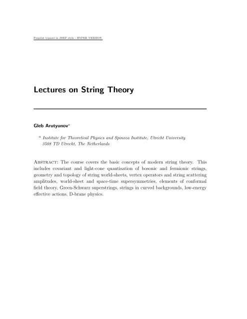
(P , X)<br />
Lm<br />
_<br />
L m<br />
_<br />
L m =0<br />
L m =0<br />
Fig. 1. The phase space of string. The Virasoro c<strong>on</strong>straints L m = 0 = ¯L m<br />
define a time-independent hypersurface <strong>on</strong> which the dynamics of string<br />
takes place. This hypersurface remains invariant under the acti<strong>on</strong> of L m ’s<br />
and ¯L m ’s.<br />
Even more generally, for any periodic functi<strong>on</strong> f we define<br />
L f =<br />
∫ 2π<br />
0<br />
dσf(σ + )T ++ .
– 23 –<br />
Then we see that<br />
0 =<br />
∫ 2π<br />
0<br />
( ) ∫ 2π ( )<br />
dσ∂ − f(σ + )T ++ = ∂ τ L f − dσ∂ σ f(σ + )T ++ .<br />
0<br />
Thus,<br />
∂ τ L f =<br />
∫ 2π<br />
0<br />
dσ∂ σ<br />
(<br />
f(σ + )T ++<br />
)<br />
= 0 .<br />
To summarize: we see that up<strong>on</strong> fixing c<strong>on</strong>formal gauge we are still left with<br />
gauge freedom. It corresp<strong>on</strong>ds to reparametrizati<strong>on</strong>s of the special type (soluti<strong>on</strong>s<br />
to the c<strong>on</strong>formal Killing equati<strong>on</strong>):<br />
σ + → ξ + (σ + ) , σ − → ξ − (σ − ) ,<br />
where ξ ± are two arbitrary functi<strong>on</strong>s periodic in σ.<br />
Finally, for the case of open string we define<br />
L m = 2T<br />
∫ π<br />
0<br />
)<br />
dσ<br />
(e imσ+ T ++ + e imσ− T −− . (3.40)<br />
The point is that there appears additi<strong>on</strong>al boundary terms which show that the old<br />
L m and ¯L m are not separately c<strong>on</strong>served. With our new definiti<strong>on</strong> of L m we obtain<br />
dL m<br />
dτ<br />
= 2T<br />
= 2T<br />
= 2T<br />
∫ π<br />
0<br />
∫ π<br />
0<br />
∫ π<br />
0<br />
)<br />
dσ<br />
(ime imσ+ T ++ + e imσ+ ∂ τ T ++ + ime imσ− T −− + e imσ− ∂ τ T −−<br />
)<br />
dσ<br />
(ime imσ+ T ++ + e imσ+ ∂ σ T ++ + ime imσ− T −− − e imσ− ∂ σ T −−<br />
)<br />
dσ<br />
(ime imσ+ T ++ − ∂ σ e imσ+ T ++ + ime imσ− T −− + ∂ σ e imσ− T −−<br />
)<br />
+ 2T e im(τ+π)( T ++ (π, τ) − e −2πim T −− (π, τ)<br />
( )<br />
− 2T e imτ T ++ (0, τ) − T −− (0, τ)<br />
The bulk term vanishes as before and we left with the boundary term<br />
dL m<br />
dτ<br />
) (<br />
)<br />
= 2T e<br />
(T im(τ+π) ++ (π, τ) − T −− (π, τ) − 2T e imτ T ++ (0, τ) − T −− (0, τ)<br />
Due to the open string boundary c<strong>on</strong>diti<strong>on</strong>s X ′µ (π, τ) = 0 = X ′µ (0, τ) we obviously<br />
have<br />
T ++ (π, τ) = T −− (π, τ) , T ++ (0, τ) = T −− (0, τ)<br />
Therefore, the boundary term vanishes and, therefore, L m are c<strong>on</strong>served quantities<br />
in the open string case.
– 24 –<br />
3.3.1 Soluti<strong>on</strong>s of the equati<strong>on</strong>s of moti<strong>on</strong><br />
Here we are going to discuss the soluti<strong>on</strong>s of the string equati<strong>on</strong>s off moti<strong>on</strong><br />
□X µ = 0<br />
which arises up<strong>on</strong> fixing the c<strong>on</strong>formal gauge.<br />
• Closed strings. We have<br />
X µ (σ, τ) = X µ L (τ + σ) + Xµ R<br />
(τ − σ)<br />
where<br />
X µ R (τ − σ) = 1 2 xµ + pµ<br />
(τ − σ) +<br />
i<br />
4πT<br />
∑<br />
√<br />
4πT<br />
n≠0<br />
n≠0<br />
1<br />
n αµ ne −in(τ−σ) (3.41)<br />
X µ L (τ + σ) = 1 2 xµ + pµ<br />
(τ + σ) +<br />
i ∑<br />
√ nᾱµ 1<br />
4πT<br />
ne −in(τ+σ) (3.42)<br />
4πT<br />
Since X µ (σ, τ) are real then (x µ , p µ ) are real as well and<br />
Let us define the zero modes as<br />
Oscillators obey the Poiss<strong>on</strong> relati<strong>on</strong>s<br />
α µ −n = (α µ n) † , ᾱ µ −n = (ᾱ µ n) †<br />
α µ 0 = ᾱ µ 0 = 1 √<br />
4πT<br />
p µ .<br />
{α µ m, α ν n} = {ᾱ µ m, ᾱ ν n} = −imδ m+n η µν ,<br />
{α µ m, ᾱ ν n} = 0 (3.43)<br />
{x µ , p ν } = η µν .<br />
The Virasoro c<strong>on</strong>straints become<br />
L m = 1 2<br />
∞∑<br />
n=−∞<br />
α µ m−nα nµ , ¯Lm = 1 2<br />
∞∑<br />
n=−∞<br />
ᾱ µ m−nᾱ nµ . (3.44)<br />
• Open strings Soluti<strong>on</strong> of the wave equati<strong>on</strong> with the open string boundary<br />
c<strong>on</strong>diti<strong>on</strong>s is<br />
X µ (σ, τ) = x µ + pµ<br />
πT τ +<br />
√ i ∑<br />
πT<br />
n≠0<br />
1<br />
n αµ ne −inτ cos nσ . (3.45)
– 25 –<br />
Oscillators obey the Poiss<strong>on</strong> algebra<br />
{α µ m, α ν n} = −imδ m+n η µν ,<br />
{x µ , p ν } = η µν . (3.46)<br />
If we define the zero mode as α µ 0 = 1 √<br />
πT<br />
p µ then the generators of the open<br />
string classical Virasoro algebra are realized as<br />
L m = 1 2<br />
∞∑<br />
n=−∞<br />
α µ m−nα nµ . (3.47)<br />
The hermiticity property of the n<strong>on</strong>-zero modes are α µ −n = (α µ n) † .<br />
3.3.2 Poincaré symmetry. <strong>String</strong> tensi<strong>on</strong>.<br />
The Noether currents of the Poincaré symmetry<br />
P α µ = −T √ −hh αβ ∂ β X µ (3.48)<br />
J µν<br />
α = −T √ −hh αβ (X µ ∂ β X ν − X ν ∂ β X µ ) (3.49)<br />
Here P α is a current corresp<strong>on</strong>ding to translati<strong>on</strong>al invariance X µ → X µ + a, where<br />
a is an arbitrary c<strong>on</strong>stant, and J µν is a current corresp<strong>on</strong>ding to Lorentz rotati<strong>on</strong>s<br />
X µ → Λ µ νX ν , where Λ µ ν is a (c<strong>on</strong>stant) matrix comprising the parameters of the<br />
Lorentz transformati<strong>on</strong>. We see that<br />
J µν<br />
α = X µ P α ν − X ν P α µ .<br />
Both currents are c<strong>on</strong>served due to equati<strong>on</strong>s of moti<strong>on</strong> of X µ and their τ-comp<strong>on</strong>ents<br />
integrated over σ define the c<strong>on</strong>served charges (for the open string case integrati<strong>on</strong><br />
rans from 0 to π)<br />
P µ =<br />
∫ 2π<br />
0<br />
dσP µ τ , J µν =<br />
∫ 2π<br />
0<br />
dσJ µν<br />
τ .<br />
Imposing the c<strong>on</strong>formal gauge and using the fundamental brackets for (X, P ) <strong>on</strong>e<br />
finds the following Poiss<strong>on</strong> algebra<br />
{P µ , P ν } = 0<br />
{P µ , J ρσ } = η µσ P ρ − η µρ P σ (3.50)<br />
{J µν , J ρσ } = η µρ J νσ + η νσ J µρ − η νρ J µσ − η µσ J νρ .<br />
Substituting soluti<strong>on</strong> for X µ <strong>on</strong>e finds<br />
P µ = T<br />
∫ 2π<br />
0<br />
dσẊµ = p µ ,
– 26 –<br />
i.e. the total mass momentum of string coincides with p µ .<br />
The total angular momentum of closed string in the c<strong>on</strong>formal gauge is is defined as<br />
J µν = T<br />
∫ 2π<br />
0<br />
Substituting the oscillator expansi<strong>on</strong> we get<br />
dσ(X µ Ẋ ν − X ν Ẋ µ ) . (3.51)<br />
where<br />
J µν = x µ p ν − x ν p µ<br />
} {{ }<br />
l µν +S µν + ¯S µν ,<br />
S µν = −i<br />
¯S µν = −i<br />
∞∑<br />
n=1<br />
∞∑<br />
n=1<br />
1 (<br />
α<br />
µ<br />
n<br />
−nαn ν − α−nα n) ν µ , (3.52)<br />
1 (ᾱµ<br />
n<br />
−nᾱn ν − ᾱ−nᾱ n) ν µ . (3.53)<br />
For the case of open string expressi<strong>on</strong>s are the same (again integrati<strong>on</strong> runs from 0 to<br />
π) except ¯S µν is absent. Here l µν is the angular momentum of string and S µν µν<br />
+ ¯S<br />
is its internal spin.<br />
Let us show that both P µ and J µν are invariant under the acti<strong>on</strong> of the Virasoro<br />
algebra. We have<br />
{L m , P µ } = {L m , p µ } = 0 (3.54)<br />
as L m does not c<strong>on</strong>tain x µ . Let us separate the zero mode part 6 of L m<br />
We first compute<br />
L m = α ρ 0α mρ + 1 2<br />
∑<br />
n≠0,m<br />
α ρ m−nα nρ .<br />
{L m , l µ } = {α ρ 0α mρ , x µ p ν − x ν p µ } = 1 √<br />
4πT<br />
α mρ {p ρ , x µ p ν − x ν p µ } =<br />
Sec<strong>on</strong>d, since S µν = − ∑ k≠0<br />
= α ν mα µ 0 − α µ mα ν 0 . (3.55)<br />
∑<br />
n,k≠0;n≠m<br />
i<br />
k αµ −k αν k<br />
we have<br />
{ 1 2 αρ m−nα nρ , − i k αµ −k αν k} = 0 ,<br />
∑<br />
{α0α ρ mρ , − i k αµ −k αν k} = α mα µ 0 ν − αmα ν µ 0 ,<br />
k≠0<br />
6 We assume here that m ≠ 0.
– 27 –<br />
therefore, {L m , l µν + S µν } = 0. Thus, Poincaré symmetry descends <strong>on</strong> the space of<br />
physical states. Physical states will be classified in terms of representati<strong>on</strong>s of the<br />
Poincaré group of d-dimensi<strong>on</strong>al Minkowski space.<br />
An important invariant of the Poincaré group is the square of the momentum P µ P µ .<br />
Indeed,<br />
{P µ P µ , P ν } = {P µ P µ , J ρλ } = 0 .<br />
It coincides with the mass: M 2 = −P µ P µ . Of course, P 2 is also invariant w.r.t. to<br />
the acti<strong>on</strong> of L m and ¯L m . C<strong>on</strong>sider now <strong>on</strong>e of the c<strong>on</strong>straints, L 0 = 0. Separating<br />
the zero mode<br />
we have<br />
L 0 = 1 2<br />
n=∞<br />
∑<br />
n=−∞<br />
From here we deduce the mass<br />
α n α −n = 1 2 α2 0 +<br />
p µ p µ + 8πT<br />
∞∑<br />
n=1<br />
α n α −n , α µ 0 = 1 √<br />
4πT<br />
p µ<br />
∞∑<br />
α n α −n = 0 .<br />
n=1<br />
M 2 = −p 2 = 8πT<br />
∞∑<br />
α n α −n .<br />
Mass is created due to internal excitati<strong>on</strong>s of string! From this expressi<strong>on</strong> it is not<br />
obvious that M 2 is n<strong>on</strong>-negative.<br />
n=1<br />
Another invariant of the Poincaré group is<br />
J 2 = 1 (<br />
J αβ J αβ + 2<br />
)<br />
2<br />
M P αJ αλ P β J 2 βλ .<br />
Checking Poincaré invariance of this expressi<strong>on</strong> is straightforward, as an intermediate step we note the relati<strong>on</strong>s<br />
{J µν , P ρ J ρσ } = η νσ J µρ P ρ − η µσ J νρ P ρ<br />
{P µ , J αβ J αβ } = −4J µρ P ρ .<br />
The terms J αβ J αβ and P αJ αλ P β J βλ separately Poiss<strong>on</strong> commute with J µν .<br />
C<strong>on</strong>sider an open string which has P i = p i = 0 for all i = 1, . . . , d − 1. By using reparametrizati<strong>on</strong> invariance fix the static<br />
gauge X 0 = τ. The angular moment l µν of this string is zero. Also P α J αλ P β J βλ = 0 and, therefore,<br />
J 2 = 1 2 J ij J ij ,<br />
where i, j = 1, . . . d − 1. We have<br />
J 2 = − 1 ∞X 1<br />
2 n,m=1 nm αi −n αj n − αj −n αi i<br />
n α −m αj m − <br />
αj −m αi m<br />
∞X 1<br />
=<br />
(α ∗ ∞X<br />
n<br />
n,m=1 nm<br />
αm)(α∗ m αn) − (α∗ n α∗ m )(αnαm) 1<br />
≤<br />
n,m=1 nm (α∗ n αm)(α∗ m αn) .
– 28 –<br />
It follows from the Schwarz inequality that<br />
(α ∗ n α m)(α ∗ m α n) = |(α ∗ n α m)| 2 ≤ (α ∗ n α n)(α ∗ m α m) ≤ nm(α ∗ n α n)(α ∗ m α m) .<br />
Therefore,<br />
∞X<br />
J 2 ≤<br />
n,m=1(α ∗ n α n)(α ∗ m α m) = 1 ∞X<br />
X ∞ 1<br />
α n α −n α m α −m =<br />
4<br />
n=−∞<br />
m=−∞<br />
(2πT ) 2 M 4<br />
because in the open string case<br />
∞X<br />
M 2 = πT α n α −n = 2πT X α n α −n .<br />
n=−∞ n>0<br />
Thus, for an open string moti<strong>on</strong> we found inequality<br />
J ≡<br />
pJ 2 ≤ 1<br />
2πT M 2 .<br />
Here the parameter<br />
α ′ = 1<br />
2πT<br />
is called a slope of the Regge trajectory. The functi<strong>on</strong> J = α ′ M 2 is a straight line in the (M 2 , J) plane whose slope is α ′ .<br />
C<strong>on</strong>sider a closed (pulsating) string soluti<strong>on</strong><br />
x = R cos σ cos τ , y = R sin σ cos τ , t = Rτ .<br />
We see that<br />
P 0 = 2πRT =⇒ T = P 0<br />
2πR ≡<br />
i.e. tensi<strong>on</strong> is energy per unit length.<br />
3.4 <strong>String</strong>s in physical gauge<br />
E<br />
2πR ,<br />
As we have seen up<strong>on</strong> fixing c<strong>on</strong>formal gauge we are still left with the gauge freedom.<br />
It corresp<strong>on</strong>ds to reparametrizati<strong>on</strong>s of the special type (soluti<strong>on</strong>s to the c<strong>on</strong>formal<br />
Killing equati<strong>on</strong>):<br />
σ + → ξ + (σ + ) , σ − → ξ − (σ − ) ,<br />
where ξ ± are two arbitrary functi<strong>on</strong>s (periodic in σ). This freedom can be further<br />
fixed leaving <strong>on</strong>ly physical excitati<strong>on</strong>s. This is achieved by imposing the so-called<br />
light-c<strong>on</strong>e gauge.<br />
3.4.1 First order formalism<br />
Introduce the light-c<strong>on</strong>e coordinates in the d-dimensi<strong>on</strong>al Minkowski space<br />
X ± = 1 √<br />
2<br />
(X 0 ± X d−1 ), X i , i = 1, . . . , d − 2 .<br />
C<strong>on</strong>sider the Polyakov acti<strong>on</strong> and introduce the light-c<strong>on</strong>e momenta c<strong>on</strong>jugate to<br />
the light-c<strong>on</strong>e coordinates<br />
P ± =<br />
∂L<br />
∂Ẋ± ,<br />
P i = ∂L<br />
∂Ẋi (3.56)
– 29 –<br />
Express now the velocities via the corresp<strong>on</strong>ding momenta<br />
Ẋ ± = 1<br />
T γ ττ (P ∓ − T γ τσ X ′± ) , Ẋ i = 1<br />
T γ ττ (−P i − T γ τσ X ′i ) .<br />
Note that the light-c<strong>on</strong>e indices are raised and lowered according to the rule<br />
P − = −P + , P + = −P − .<br />
Now we can c<strong>on</strong>struct the phase-space Lagrangian in the light-c<strong>on</strong>e coordinates:<br />
After explicit computati<strong>on</strong> we find<br />
L = P i Ẋ i + P + Ẋ + + P − Ẋ − + rest .<br />
L = P i Ẋ i + P + Ẋ + + P − Ẋ − + 1<br />
2T γ ττ (<br />
− 2P − P + + P i P i + T 2 X ′ iX ′i − 2T 2 X ′− X ′+ )<br />
+ γτσ<br />
γ ττ (<br />
P i X ′i + P − X ′− + P + X ′+ )<br />
. (3.57)<br />
The phase-space light-c<strong>on</strong>e gauge c<strong>on</strong>sists in imposing the following two c<strong>on</strong>diti<strong>on</strong>s<br />
1. Closed string<br />
2. Open string<br />
X + = p+<br />
2πT τ , P + = c<strong>on</strong>st ≡ 1<br />
2π p+ . (3.58)<br />
X + = p+<br />
πT τ , P + = c<strong>on</strong>st ≡ 1 π p+ . (3.59)<br />
This gauge choice is d<strong>on</strong>e to remove completely the gauge degrees of freedom (recall<br />
that in the c<strong>on</strong>formal gauge we still had a gauge freedom left which was generated<br />
by soluti<strong>on</strong>s of the c<strong>on</strong>formal Killing equati<strong>on</strong>).<br />
We further c<strong>on</strong>sider the closed string case in detail. We will derive and solve all<br />
the c<strong>on</strong>straints followed from the Lagrangian (3.57) in several steps.<br />
1. Varying the Lagrangian w.r.t. γ ττ and imposing the light-c<strong>on</strong>e gauge allows<br />
<strong>on</strong>e to solve for P − :<br />
P − = π (<br />
)<br />
P<br />
p + i P i + T 2 X iX ′ ′i . (3.60)<br />
Thus, equati<strong>on</strong> of moti<strong>on</strong> for γ ττ allows <strong>on</strong>e to determine P − .
– 30 –<br />
2. Varying w.r.t. γ τσ leads to determinati<strong>on</strong> of X ′− :<br />
X ′− = − 1<br />
P −<br />
P i X ′i = 2π<br />
p + P iX ′i . (3.61)<br />
If we integrate the last equati<strong>on</strong> over σ we obtain<br />
X − (2π) − X − (0) = 2π<br />
p + ∫ 2π<br />
0<br />
dσP i X ′i . (3.62)<br />
The closed string periodicity c<strong>on</strong>diti<strong>on</strong> requires the fulfillment of the following<br />
c<strong>on</strong>straint<br />
V =<br />
∫ 2π<br />
0<br />
dσP i X ′i = 0 . (3.63)<br />
This is the <strong>on</strong>ly c<strong>on</strong>straint which remains unsolved and it is known as the level<br />
matching c<strong>on</strong>diti<strong>on</strong>. We will impose it <strong>on</strong> physical states of the theory.<br />
3. Now we can determine the world-sheet metric γ αβ . Equati<strong>on</strong> of moti<strong>on</strong> for P +<br />
is<br />
0 = δL =<br />
δP Ẋ+ −<br />
P − γτσ<br />
+<br />
+ T γττ γ ττ X′+ ,<br />
which with our gauge choice gives<br />
γ ττ = −1 .<br />
4. Equati<strong>on</strong> of moti<strong>on</strong> for Ẋ− gives<br />
which gives<br />
0 = d δL δL<br />
−<br />
dt δẊ− δX = − d p +<br />
− dt 2π − δL δL<br />
=⇒<br />
δX− δX = 0 , −<br />
( ) γ<br />
τσ<br />
∂ σ<br />
γ P ττ − = 0 =⇒ ∂ σ γ τσ = 0 .<br />
For the closed string case this implies that γ τσ = γ τσ (τ) is an arbitrary functi<strong>on</strong><br />
of τ. The presence of this functi<strong>on</strong> signals a residual symmetry. Indeed, <strong>on</strong> the<br />
soluti<strong>on</strong>s of the level-matching c<strong>on</strong>straint V = 0 the ratio γτσ<br />
can be shifted by<br />
γ ττ<br />
an arbitrary functi<strong>on</strong> f(τ) of τ without affecting the Lagrangian.<br />
5. Varying w.r.t P − we find an evoluti<strong>on</strong> equati<strong>on</strong> for X − :<br />
0 = δL<br />
δP −<br />
= Ẋ− − P +<br />
T γ ττ = 0 =⇒ Ẋ− = π<br />
T p + (P iP i + T 2 X ′ iX ′i ) .
– 31 –<br />
Thus, the variable X − is not physical and can be solved from the following two<br />
equati<strong>on</strong>s we found above<br />
Ẋ − =<br />
These two equati<strong>on</strong>s can be rewritten as<br />
π<br />
T p + (P iP i + T 2 X ′ iX ′i ) (3.64)<br />
X ′− = 2π<br />
p + P iX ′i (3.65)<br />
∂ ± X − = 2πT<br />
p + (∂ ±X i ) 2 . (3.66)<br />
It is worth noting that two equati<strong>on</strong>s (3.64), (3.65) are compatible. Indeed, the<br />
σ-derivative of the first equati<strong>on</strong> must be equal the τ-derivative of the sec<strong>on</strong>d<br />
<strong>on</strong>e. One can see that this is indeed so due to equati<strong>on</strong>s of moti<strong>on</strong> for physical<br />
fields.<br />
Now we are ready to c<strong>on</strong>struct the gauge-fixed Lagrangian. Substituting soluti<strong>on</strong>s<br />
of all the c<strong>on</strong>straints and the gauge c<strong>on</strong>diti<strong>on</strong>s into eq.(3.57) we obtain the density<br />
L = P i Ẋ i − 1<br />
)<br />
2π p+ Ẋ − − p+<br />
2πT P − − γ τσ (τ)<br />
(P i X ′i − p+<br />
2π X′− . (3.67)<br />
Thus, the Lagrangian itself is<br />
L =<br />
∫ 2π<br />
0<br />
∫ 2π<br />
dσL = −p + ẋ − + dσ P i Ẋ i −H − γ τσ (τ)V . (3.68)<br />
0<br />
} {{ }<br />
defines Poiss<strong>on</strong> structure<br />
Here x − denotes the zero (c<strong>on</strong>stant) mode of the variable X − and the Hamilt<strong>on</strong>ian<br />
is<br />
H = 1 ∫ 2π<br />
)<br />
dσ<br />
(P i P i + T 2 X ′<br />
2T<br />
iX ′i .<br />
0<br />
We also see that γ τσ (τ) plays the role of the Lagrangian multiplier to the levelmatching<br />
c<strong>on</strong>straint V. Without loss of generality we will choose γ τσ = 0 which<br />
corresp<strong>on</strong>ds the c<strong>on</strong>formal gauge c<strong>on</strong>diti<strong>on</strong> discussed above.<br />
From the gauge-fixed Lagrangian we c<strong>on</strong>clude that our physical variables are (P i , X i ),<br />
where i = 1, . . . , d−2, and also (x − , p + ) and they have the following Poiss<strong>on</strong> brackets<br />
{X i (σ, τ), X j (σ ′ , τ)} = {P i (σ, τ), P j (σ ′ , τ)} = 0 ,<br />
{X i (σ, τ), P j (σ ′ , τ)} = δ ij δ(σ − σ ′ ) , (3.69)<br />
{p + , x − } = 1 .
– 32 –<br />
The physical Hamilt<strong>on</strong>ian and the Poiss<strong>on</strong> brackets look the same as the <strong>on</strong>es in the<br />
c<strong>on</strong>formal gauge, however, the important difference is that now they involve 2(d − 2)<br />
physical fields <strong>on</strong>ly plus two additi<strong>on</strong>al degrees of freedom (x − , p + ). First, from<br />
eq.(3.65) we find that the zero mode of X − evolves as<br />
ẋ − = 1<br />
p + H =⇒ x− (τ) = x − + H p + τ .<br />
It is this τ-independent mode x − which is c<strong>on</strong>jugate to p + . Sec<strong>on</strong>d, equati<strong>on</strong>s<br />
∂ ± X − = 2πT<br />
p + (∂ ±X i ) 2 (3.70)<br />
can be solved for the l<strong>on</strong>gitudinal oscillators αn − , ᾱn<br />
− with n ≠ 0 by substituting an<br />
expansi<strong>on</strong><br />
X − (τ, σ) = x − + p−<br />
}{{} 2πT<br />
τ + i<br />
p + H<br />
We find p − = 2πT<br />
p + H and<br />
√<br />
4πT<br />
∑<br />
n≠0<br />
1<br />
(<br />
αn − e −inσ− + ᾱn − e −inσ+) . (3.71)<br />
n<br />
α − n =<br />
ᾱ − n =<br />
√<br />
πT<br />
p +<br />
√<br />
πT<br />
p +<br />
∞<br />
∑<br />
m=−∞<br />
∑ ∞<br />
m=−∞<br />
α i n−mα i m , n ≠ 0, (3.72)<br />
ᾱ i n−mᾱ i m , n ≠ 0 . (3.73)<br />
These formulae give a complete soluti<strong>on</strong> for X − .<br />
Thus, the light-c<strong>on</strong>e gauge allows for the explicit soluti<strong>on</strong> of the Virasoro c<strong>on</strong>straints.<br />
The variables (P i , X i ) are physical excitati<strong>on</strong>s while X ± , P + were removed by the<br />
light-c<strong>on</strong>e gauge choice and by solving the c<strong>on</strong>straints. The variable P − plays the<br />
role of the Hamilt<strong>on</strong>ian for physical excitati<strong>on</strong>s! Equati<strong>on</strong>s of moti<strong>on</strong> for physical<br />
fields are the same as before<br />
Ẍ i − X ′′i = 0 , i = 1, . . . , d − 2.<br />
The variables (P i , X i ), where i = 1, . . . , d − 2, are called transversal, while X ± , P ±<br />
are l<strong>on</strong>gitudinal. The <strong>on</strong>ly c<strong>on</strong>straint which we were not able to solve explicitly is<br />
the level-matching c<strong>on</strong>straint V = 0. It is easy to check that<br />
{X i , V} = ∂ σ X i , {P i , V} = ∂ σ P i , (3.74)<br />
i.e. V generates the rigid σ-rotati<strong>on</strong>s. We also have the evoluti<strong>on</strong> equati<strong>on</strong>s<br />
{X i , H} = 1 T P i = ∂ τ X i , {P i , H} = T ∂ 2 σX i = ∂ τ P i . (3.75)
– 33 –<br />
One can also see that the τ- and σ-flows generated by H and V respectively commute<br />
with each other because<br />
{H, V} = 0 .<br />
Impositi<strong>on</strong> of the light-c<strong>on</strong>e gauge is possible because in the c<strong>on</strong>formal gauge the<br />
field X + satisfies the wave equati<strong>on</strong>: □X + = 0. The corresp<strong>on</strong>ding soluti<strong>on</strong> for X +<br />
is<br />
X + (τ, σ) = x + + p+<br />
2πT τ +<br />
√ i ∑<br />
4πT<br />
n≠0<br />
1<br />
(<br />
α n + e −inσ− + ᾱ n + e −inσ+) . (3.76)<br />
n<br />
Our gauge choice (3.58) is taken to be compatible with the form (3.76). Effectively,<br />
it means taken equal to zero all oscillators<br />
α + n = 0 = ᾱ + n , n ≠ 0<br />
and also x + = 0 or<br />
α + n = ᾱ + n = p+<br />
√<br />
4πT<br />
δ n,0 .<br />
One may w<strong>on</strong>der why <strong>on</strong>e cannot completely remove X + , i.e. to choose a gauge<br />
X + = 0. To understand this point <strong>on</strong>e has to remember that the infinitesimal<br />
c<strong>on</strong>formal transformati<strong>on</strong>s are of the form<br />
X → X + ∑ n<br />
a n e inσ− ∂ − X ,<br />
X → X + ∑ n<br />
ā n e inσ+ ∂ + X ,<br />
where a n , ā n are arbitrary c<strong>on</strong>stants. In other words these transformati<strong>on</strong>s can be<br />
written as<br />
X → X + ξ − (σ − ) , X → X + ξ + (σ + ) ,<br />
where ξ ± are arbitrary functi<strong>on</strong>s obeying <strong>on</strong>ly <strong>on</strong>e requirement: they must be periodic<br />
in σ. These functi<strong>on</strong>s can be used to remove all oscillator modes and the zero mode<br />
x + but they cannot remove<br />
p + τ = p+ 2 (τ − σ) + p+ 2<br />
(τ + σ)<br />
because the functi<strong>on</strong>s τ − σ and τ + σ are not periodic in σ.<br />
<strong>String</strong> in the light-c<strong>on</strong>e gauge can be treated in the standard framework of the Hamilt<strong>on</strong>ian reducti<strong>on</strong>.<br />
H = L 0 + ¯L 0 is invariant under the symmetry algebra <strong>on</strong> the surface L m = 0 = ¯L m :<br />
The Hamilt<strong>on</strong>ian<br />
{H, L m} = imL m , {H, ¯L m} = im ¯L m .<br />
The symmetry algebra itself is<br />
{L n, L m} = −i(m − n)L n+m , { ¯L n, ¯L m} = −i(m − n) ¯L n+m .
– 34 –<br />
Orbits of the Virasoro algebra<br />
+<br />
Gauge c<strong>on</strong>diti<strong>on</strong> for X<br />
C<strong>on</strong>strained surface<br />
_<br />
L m =L m =0<br />
Phase space (P,X)<br />
Fig. 2. The physical phase space is obtained by solving the Virasoro c<strong>on</strong>straints<br />
L m = 0 = ¯L m and reducing the acti<strong>on</strong> of the Virasoro algebra <strong>on</strong><br />
the c<strong>on</strong>strained surface by imposing the light-c<strong>on</strong>e gauge.<br />
One would like to reduce the dynamics of the system over the acti<strong>on</strong> of the symmetry algebra.<br />
Hamilt<strong>on</strong>ian reducti<strong>on</strong> c<strong>on</strong>diti<strong>on</strong>s<br />
L m = 0 = ¯L m<br />
In the framework of the<br />
corresp<strong>on</strong>d to fixing the moment map. The reduced phase space P is defined as a quotient space<br />
P = soluti<strong>on</strong>s of L m = 0 = ¯L m<br />
isotropy subalgebra<br />
,<br />
where the isotropy subalgebra is a subalgebra of the Virasoro algebra which leaves the surface L m = 0 = ¯L m invariant. In our present<br />
situati<strong>on</strong> this subalgebra coincides with the algebra itself and, therefore,<br />
P = soluti<strong>on</strong>s of Lm = 0 = ¯L m<br />
acti<strong>on</strong> of Virasoro<br />
.<br />
The acti<strong>on</strong> of the Virasoro algebra is factored out by imposing the light-c<strong>on</strong>e gauge, which simultaneously leads to solving the Virasoro<br />
c<strong>on</strong>straints. The transversal coordinates introduced above provide the descripti<strong>on</strong> of the reduced phase space.<br />
Mass of the string in the light-c<strong>on</strong>e gauge is computed as follows (recall that mass<br />
is a quadratic Casimir of the Poincaré group). Since we have found that p − = 2πT H<br />
p +<br />
we get for the mass<br />
The physical Hamilt<strong>on</strong>ian is<br />
H = 1 2<br />
Thus, we obtain<br />
M 2 = −p µ p µ = −(p i ) 2 + 2p + p − = −(p i ) 2 + 4πT H . (3.77)<br />
∞∑<br />
n=−∞<br />
(<br />
α<br />
i<br />
n α i −n + ᾱ i nᾱ i −n)<br />
=<br />
(p i ) 2<br />
4πT + ∞<br />
∑<br />
n=1<br />
( )<br />
α<br />
i<br />
n α−n i + ᾱnᾱ i −n<br />
i . (3.78)<br />
M 2 = 4πT<br />
∞∑<br />
n=1<br />
(<br />
α<br />
i<br />
n α i −n + ᾱ i nᾱ i −n)<br />
=<br />
2<br />
α ′<br />
∞<br />
∑<br />
n=1<br />
( )<br />
α<br />
i<br />
n α−n i + ᾱnᾱ i −n<br />
i . (3.79)<br />
This clearly shows positivity of M 2 , a property which was not obvious in the c<strong>on</strong>formal<br />
gauge.
– 35 –<br />
Finally, we can write the level-matching c<strong>on</strong>diti<strong>on</strong> in terms of transversal oscillators.<br />
We find<br />
V = 1 ∑ (<br />
)<br />
ᾱ i<br />
2T<br />
nᾱ−n i − αnα i −n<br />
i = 0 . (3.80)<br />
n≠0<br />
Thus, the level-matching c<strong>on</strong>diti<strong>on</strong> tells that the left- and right-moving oscillators<br />
c<strong>on</strong>tribute the same amount of energy.<br />
3.4.2 Poiss<strong>on</strong> structure of the light-c<strong>on</strong>e theory<br />
Using the Poiss<strong>on</strong> brackets of physical fields we can now establish the Poiss<strong>on</strong> relati<strong>on</strong>s<br />
between all quantities of interest. We first summarize the basic Poiss<strong>on</strong> relati<strong>on</strong>s<br />
for the closed string case<br />
{, } p + p − p j x j x − αm j αm<br />
−<br />
p + 0 0 0 0 1 0 0<br />
p − 0 0 0 − pi<br />
− p− 2πiT<br />
mα j 2πiT<br />
p + p + p + m mα − p + m<br />
p i 0 0 0 − δ ij 0 0 0<br />
x i 0<br />
x − − 1<br />
p i<br />
δ ij δ<br />
0 0 ij δ m<br />
p + 4πT<br />
p −<br />
0 0 0 0<br />
p +<br />
α i n 0 − 2πiT<br />
p + nα i n 0 − δij δ n<br />
αn − 0 − 2πiT nα − p + n 0 − αi n<br />
p +<br />
4πT<br />
0 − inδ ij δ n+m − i √ 4πT<br />
− α− n<br />
p +<br />
α i m<br />
p +<br />
α − m<br />
p +<br />
nα i p + n+m<br />
i √ 4πT<br />
p + mα i n+m {α − n , α − m}<br />
Tab. 1. Poiss<strong>on</strong> brackets of the light-c<strong>on</strong>e modes. The variable p − is<br />
essentially the Hamilt<strong>on</strong>ian: p − = 2πT H . The brackets involving ᾱ<br />
p +<br />
variables are the same.<br />
These relati<strong>on</strong>s are easy to derive. For instance,<br />
{p − , x − } = {2πT H p + , x− } = −2πT H 1<br />
(p + ) 2 {p+ , x − } = −2πT H<br />
(p + ) 2 = −p− p + .<br />
Also, <strong>on</strong>e has to remember that the variable α − n c<strong>on</strong>tains the zero mode α i 0<br />
α − n =<br />
√<br />
πT<br />
p +<br />
2αi 0α i n + . . . = pi α i n<br />
p + + . . .<br />
and, therefore,<br />
{x i , α − n } = 1<br />
p + {xi , p j α j n} = 1<br />
p + αi n .<br />
The most complicated bracket is {α − m, α − n }.
– 36 –<br />
Let us outline the computati<strong>on</strong> of this bracket.<br />
{α − m , α− n } = n p<br />
i α<br />
i<br />
m<br />
p +<br />
n p<br />
i α<br />
i<br />
m<br />
p +<br />
, pj α j o<br />
n<br />
p + +<br />
+ √<br />
πT<br />
p +<br />
√<br />
πT<br />
p +<br />
X<br />
k≠m,0<br />
α i m−k αi k , pj α j n<br />
p +<br />
n p<br />
i α<br />
i<br />
m<br />
p + , X<br />
α j o<br />
n−l αj −<br />
l<br />
l≠n,0<br />
√<br />
πT<br />
+ 2πT<br />
−im pi p i<br />
(p + ) 2 δ n+m −2i(m − n)<br />
(p + ) 2 pi α i n+m<br />
| {z } | {z }<br />
first bracket sec<strong>on</strong>d and third brackets<br />
√<br />
πT<br />
+ X<br />
p + α j o<br />
n−l αj =<br />
l<br />
l≠n,0<br />
√<br />
πT n p<br />
i α<br />
i<br />
n<br />
p + p + , X<br />
α j o<br />
m−l αj + πT n X<br />
l<br />
(p<br />
l≠m,0<br />
) 2 α i m−k αi k ,<br />
X<br />
α j o<br />
n−l αj l<br />
k≠m,0<br />
l≠n,0<br />
0<br />
1<br />
X<br />
@−i(m<br />
(p + ) 2 − n)<br />
α i n+m−k αi A<br />
k .<br />
k≠m+n,0<br />
(3.81)<br />
| {z }<br />
forth bracket<br />
Thus, we are getting<br />
0<br />
1<br />
{α − m , α− n } = −im pi p i<br />
(p + ) 2 δ n+m + 2πT<br />
∞X<br />
@−i(m<br />
(p + ) 2 − n) α i n+m−k αi A<br />
k ,<br />
k=−∞<br />
where due to α i 0 = √ pi we combined the sec<strong>on</strong>d and a third terms into <strong>on</strong>e sum. If m + n ≠ 0 then the first term vanishes and we<br />
4πT<br />
can rewrite the last formula as<br />
{α − m , α− n } = √<br />
4πT<br />
p +<br />
<br />
−i(m − n)α − <br />
m+n .<br />
If n = −m then in eq.(3.81) c<strong>on</strong>tributi<strong>on</strong> from the sec<strong>on</strong>d and the third term vanishes and we get<br />
0<br />
1<br />
{α − m , α− −m } = −im pi p i<br />
(p + ) 2 + 2πT @−2im X √ 0 √<br />
(p + ) 2 α i 4πT πT h p i ! 2<br />
−k αi A<br />
k ≡ −2im @<br />
p<br />
k≠0<br />
+ p + √ + X α i k −ki 1<br />
αi A .<br />
4πT<br />
k≠0<br />
Therefore,<br />
√ 0 √<br />
{α − 4πT πT<br />
m , α− −m } = −2im @<br />
p + p +<br />
1<br />
X ∞ α i k αi A<br />
−k .<br />
k=−∞<br />
It is therefore natural to define<br />
α − 0<br />
≡ √<br />
πT<br />
p +<br />
∞ X<br />
k=−∞<br />
α i k αi −k .<br />
With this definiti<strong>on</strong> we obtained a universal formula (valid for all indices m and n):<br />
{α − m , α− n } = √<br />
4πT<br />
p +<br />
<br />
−i(m − n)α − <br />
m+n .<br />
Also we c<strong>on</strong>clude that with this definiti<strong>on</strong><br />
p − = √ πT (α − 0 + ᾱ− 0 ) .<br />
Thus, <strong>on</strong>e finds the following result<br />
{α − m, α − n } =<br />
√<br />
4πT<br />
p + (<br />
−i(m − n)α<br />
−<br />
m+n<br />
)<br />
.<br />
If we introduce<br />
L n = p+<br />
√<br />
4πT<br />
α − n .<br />
we therefore find<br />
{L n , L m } = −i(n − m)L n+m<br />
which is the classical Virasoro algebra! Thus, in the light-c<strong>on</strong>e gauge the Virasoro<br />
algebra is carried over by the l<strong>on</strong>gitudinal oscillators α − n .
– 37 –<br />
3.4.3 Lorentz symmetry<br />
The light-c<strong>on</strong>e gauge manifestly breaks the d-dimensi<strong>on</strong>al Lorentz invariance of the<br />
theory. We have the generators of the Lorentz algebra which in terms of transversal<br />
oscillators become realized n<strong>on</strong>-linearly. For instance, the generator<br />
∞∑<br />
J i− = x i p − − x − p<br />
} {{ }<br />
i −i<br />
l i−<br />
n=1<br />
1 ( ∑ ∞<br />
α<br />
i<br />
n −n αn − − α−nαn) − i − i<br />
n=1<br />
1 (ᾱi<br />
n −n ᾱn − − ᾱ−nᾱn)<br />
− i<br />
is not anymore quadratic in oscillators because p − and α − are n<strong>on</strong>-trivial functi<strong>on</strong><br />
of the transversal oscillators.<br />
In spite of rather n<strong>on</strong>-linear realizati<strong>on</strong> <strong>on</strong>e can check that all the Poiss<strong>on</strong> relati<strong>on</strong>s<br />
involving J i− are still satisfied (this is also c<strong>on</strong>sequence of the fact that<br />
{L m , J µν } = 0 = {¯L m , J µν } , which means that the Poiss<strong>on</strong> bracket of J µν admits a<br />
reducti<strong>on</strong> <strong>on</strong> the c<strong>on</strong>straint surface L m = 0 = ¯L m ). In particular, from the Poincaré<br />
algebra we must have<br />
{J i− , J j− } = 0 .<br />
Let us check this explicitly. First we have<br />
{l i− , l j− } = {x i p − − x − p i , x j p − − x − p j } =<br />
= {x i p − , x j p − } − {x − p i , x j p − } − {x i p − , x − p j } + {x − p i , x − p j } .<br />
By using the Poiss<strong>on</strong> brackets from Table 1 we obtain<br />
{l i− , l j− } = pi<br />
p + p− x j − pj<br />
p + p− x i −p i x j p−<br />
p + + x− p − δ ij<br />
| {z }<br />
first bracket<br />
| {z }<br />
sec<strong>on</strong>d bracket<br />
+p j x i p−<br />
p + − x− p − δ ij<br />
| {z }<br />
third bracket<br />
.<br />
and the forth bracket vanishes. Thus,<br />
{l i− , l j− } = 0 .<br />
C<strong>on</strong>sider the Poiss<strong>on</strong> bracket of the internal spin comp<strong>on</strong>ents<br />
{S i− , S j− } = − X 1<br />
nm {αi −n α− n , αj −m α− m } =<br />
n,m≠0<br />
= − X 1 <br />
{α i <br />
−n<br />
nm<br />
, αj −m }α− n α− m + {αi −n , α− m }α− n αj −m + {α− n , αj −m }αi −n α− m + {α− n , α− m }αi −n αj −m<br />
=<br />
n,m≠0<br />
= iδ ij X α − √<br />
n α− −n 4πT X<br />
<br />
+ i<br />
n p<br />
n≠0<br />
+<br />
− 1 m αi −n+m αj −m α− n + 1 n αi −n αj n−m α− m + n − m<br />
<br />
nm<br />
αi −n αj −m α− m+n .<br />
m,n≠0<br />
Here the first first sum is zero (proved by changing n for −n). In the sec<strong>on</strong>d and the third summ<strong>on</strong>ds <strong>on</strong>e makes the change of<br />
summati<strong>on</strong> indices, n → n + m and m → m + n respectively. After this change these terms cancel exactly against the last <strong>on</strong>e.<br />
However, there are terms which are still left, these are the terms in the sec<strong>on</strong>d and third summ<strong>on</strong>ds c<strong>on</strong>taining zero modes, i.e. terms<br />
for which −n + m = 0 and also the term of the last summ<strong>on</strong>d for which m + n = 0 . Thus,<br />
{S i− , S j− } = − i<br />
√<br />
X 1 <br />
p + p i α j −n<br />
n<br />
− pj α i −n<br />
α − 4πT<br />
n + 2i X 1<br />
p<br />
n≠0<br />
+ α− 0<br />
n αi n αj −n . (3.82)<br />
n≠0<br />
Analogously, we will get the following c<strong>on</strong>tributi<strong>on</strong> from the left-moving modes Then we compute<br />
{l i− , S j− } = −i X 1<br />
n {xi p − − x − p i , α j −n<br />
| {z } | {z }<br />
α− n } = −i X 1<br />
n B<br />
α j n≠0<br />
n≠0 @<br />
−n p− αin<br />
p + + xi − 2πiT<br />
p + nαj −n α− n + 2πiT<br />
<br />
p + nαj −n α− n<br />
A B<br />
| {z }<br />
from A<br />
0<br />
− p i α j α − n<br />
−n<br />
p +<br />
| {z }<br />
from B<br />
1<br />
.<br />
C<br />
A
– 38 –<br />
Thus, we arrive at<br />
{l i− , S j− } + {S i− , l j− } = −2i p− X 1<br />
p + n αi n αj −n +<br />
i X 1 <br />
p<br />
n≠0<br />
+ p i α j −n<br />
n<br />
− pj α i <br />
−n α − n . (3.83)<br />
n≠0<br />
Now summing up equati<strong>on</strong>s (3.82) and (3.83) we obtain<br />
{l i− , S j− } + {S i− , l j− } + {S i− , S j− } = i 4√ πT<br />
p +<br />
<br />
α − 0 − α− 0 + ᾱ− X<br />
0<br />
2<br />
n≠0<br />
1<br />
n αi n αj −n . (3.84)<br />
At first glance this expressi<strong>on</strong> is n<strong>on</strong>-zero and it can not be compensated by the c<strong>on</strong>tributi<strong>on</strong> of left-moving modes<br />
{l i− , ¯S j− } + { ¯S i− , l j− } + { ¯S i− , ¯S j− } = i 4√ πT<br />
p +<br />
<br />
ᾱ − 0 − α− 0 + ᾱ− X<br />
0<br />
2<br />
n≠0<br />
1<br />
n ᾱi nᾱj −n . (3.85)<br />
However, we have to invoke the level-matching c<strong>on</strong>straint which simply tells that α − 0 = ᾱ− 0<br />
and makes both eqs.(3.84) and (3.85)<br />
separately vanish. Thus, we have indeed shown that the most n<strong>on</strong>-trivial relati<strong>on</strong> {J i− , J j− } = 0 is indeed satisfied.<br />
4. Quantizati<strong>on</strong> of bos<strong>on</strong>ic string<br />
4.1 Remarks <strong>on</strong> can<strong>on</strong>ical quantizati<strong>on</strong><br />
According to the standard principles of quantum mechanics can<strong>on</strong>ical quantizati<strong>on</strong><br />
c<strong>on</strong>sists in replacing the Poiss<strong>on</strong> brackets of the fundamental phase space variables<br />
by commutators<br />
{ , } → 1<br />
i [ , ] ,<br />
where is the Plank c<strong>on</strong>stant. Thus, we c<strong>on</strong>sider now X(σ, τ) and P (σ, τ) as the<br />
quantum mechanical operators which obey the following commutati<strong>on</strong> relati<strong>on</strong>s 7<br />
[X µ (σ, τ), X ν (σ ′ , τ)] = [P µ (σ, τ), P ν (σ ′ , τ)] = 0 ,<br />
[X µ (σ, τ), P ν (σ ′ , τ)] = iη µν δ(σ − σ ′ ) , (4.1)<br />
These commutati<strong>on</strong> relati<strong>on</strong>s induce the commutati<strong>on</strong> relati<strong>on</strong>s <strong>on</strong> the Fourier coefficients<br />
[α µ m, α ν n] = [ᾱ µ m, ᾱ ν n] = mδ m+n η µν ,<br />
[α µ m, ᾱ ν n] = 0 , (4.2)<br />
[x µ , p ν ] = iη µν .<br />
For the case of open string the modes ᾱ n are absent. In what follows we will work<br />
in units in which = 1, so that the commutati<strong>on</strong> relati<strong>on</strong>s read as<br />
[α µ m, α ν n] = [ᾱ µ m, ᾱ ν n] = mδ m+n η µν ,<br />
[α µ m, ᾱ ν n] = 0 , (4.3)<br />
[x µ , p ν ] = iη µν .<br />
7 Here the indices µ, ν run from 0 to d − 1.
– 39 –<br />
To restore , <strong>on</strong>e has to simply rescale the modes as α → 1 √<br />
~<br />
α, ᾱ → 1 √<br />
~ ᾱ.<br />
Let us take m > 0 and rescale a m = 1 √ m<br />
α m . Then using the hermiticity property<br />
the commutati<strong>on</strong> relati<strong>on</strong>s can be rewritten as<br />
[a µ n, a †ν<br />
m] = η µν δ n,m<br />
[ā µ n, ā †ν<br />
m] = η µν δ n,m<br />
which are the standard commutati<strong>on</strong> relati<strong>on</strong>s of two infinite sets of independent<br />
quantum harm<strong>on</strong>ic oscillators.<br />
Introduce the number operator for m’s mode<br />
Then we see that for m > 0<br />
From here we c<strong>on</strong>clude that<br />
N m =: α µ mα −m,µ :<br />
[N m , α m ] = −mα m ,<br />
[N m , α −m ] = mα −m .<br />
• Modes with m > 0 should be identified with the lowering operators<br />
• Modes with m < 0 should be identified with the raising operators<br />
C<strong>on</strong>structi<strong>on</strong> of the representati<strong>on</strong> of the can<strong>on</strong>ical commutati<strong>on</strong> relati<strong>on</strong>s is completed<br />
by introducing the ground state which satisfies the following properties<br />
α µ m|p ν 〉 = 0 ,<br />
ˆp µ |p ν 〉 = p µ |p ν 〉 . (4.4)<br />
The whole infinite-dimensi<strong>on</strong>al (Hilbert) space of states is obtained by acting <strong>on</strong> the<br />
ground state with creati<strong>on</strong> operators.<br />
This c<strong>on</strong>structi<strong>on</strong> brings us to the major problem of can<strong>on</strong>ical quantizati<strong>on</strong>.<br />
C<strong>on</strong>sider for m positive the following commutator<br />
[α 0 m, α 0 −m] = [α 0 m, (α 0 m) † ] = mη 00 = −m .<br />
Thus, we induce from here (let even a ground state carries zero momentum p µ )<br />
〈0|[α 0 m, (α 0 m) † ]|0〉 = 〈0|α 0 m (α 0 m) † |0〉 = ||(α 0 m) † |0〉|| 2 = −m < 0 .<br />
Thus, Minkowskian type of the target-space metric leads to the existence in the<br />
Hilbert space the states with negative norm. States with negative norm are sometimes<br />
called “ghosts” and they do not allow for probability interpretati<strong>on</strong> of the<br />
corresp<strong>on</strong>ding quantum-mechanical system.
– 40 –<br />
One can correctly anticipate that the problem with negative norm states arose<br />
because we did not take into account the Virasoro c<strong>on</strong>straints. The covariant approach<br />
to quantizati<strong>on</strong> c<strong>on</strong>sists in defining the subspace of physical states in the<br />
original Hilbert space which obey the Virasoro c<strong>on</strong>straints. One can further show<br />
that in a special dimensi<strong>on</strong> of space-time (d = 26) the negative norm states decouple<br />
from the physical Hilbert space.<br />
In the classical theory we have the c<strong>on</strong>straints L m = 0 = ¯L m . However, in<br />
quantum theory expressi<strong>on</strong>s for L m and ¯L m are quadratic in oscillators and might<br />
involve operators (quantum oscillators) which do not commute with each other! From<br />
all L m a c<strong>on</strong>straint which suffers from ordering ambiguity is L 0 as<br />
L 0 = 1 2<br />
∞∑<br />
n=−∞<br />
α µ nα −n,µ (4.5)<br />
and oscillators α n µ and α µ −n do not commute with each other. The standard way<br />
to deal with this ambiguity in quantum field theory is to use the normal ordering<br />
prescripti<strong>on</strong><br />
L m = 1 2<br />
∞∑<br />
n=−∞<br />
The normal ordering prescripti<strong>on</strong> means that<br />
: α m1 . . . α mk := α n1 . . . α np<br />
} {{ }<br />
all creati<strong>on</strong><br />
: α µ m−nα n,µ : . (4.6)<br />
α s1 . . . α sr<br />
} {{ }<br />
all annihilati<strong>on</strong><br />
in the operators are ordered in such a fashi<strong>on</strong> that all annihilati<strong>on</strong> operators are<br />
put <strong>on</strong> the right from all the creati<strong>on</strong> operators. The order of the creati<strong>on</strong> (or<br />
annihilati<strong>on</strong>) operators between themselves does not matter because these operators<br />
commute between themselves and therefore their expressi<strong>on</strong> does not have ordering<br />
ambiguity. In particular, for L 0 we have<br />
L 0 = 1 2 α2 0 +<br />
∞∑<br />
α −nα µ n,µ − a , (4.7)<br />
n=1<br />
where we include a so far unknown normal ordering c<strong>on</strong>stant a. As to the zero modes,<br />
the normal-ordering prescripti<strong>on</strong> here is<br />
: p µ x ν := x ν p µ .<br />
Since the ground state obeys ˆp µ |p〉 = p µ |p〉 it can be regarded as the usual quantummechanical<br />
eigenstate of the momentum operator ˆp µ = −i ∂<br />
∂x µ<br />
which is in the momentum<br />
representati<strong>on</strong> has the form of the plane-wave<br />
|p〉 ≡ e ipµ x µ<br />
|0〉 ,
– 41 –<br />
where <strong>on</strong> the r.h.s. p µ is not an operator and |0〉 denotes the zero-momentum ground<br />
state. Plane-waves are not square-integrable functi<strong>on</strong>s but they form a basis of a<br />
generalized Hilbert space and they are assumed to be normalized as<br />
〈p|p ′ 〉 = δ(p − p ′ ) .<br />
4.1.1 Virasoro algebra<br />
Let us now investigate the algebra of the operators L m in the quantum case. We<br />
first assume that the normal ordering c<strong>on</strong>stant a = 0. We start by computing<br />
∞∑<br />
∞∑<br />
)<br />
[α m, µ L n ] = 1 [α µ 2 m, : αpα ν n−p,ν :] =<br />
(mδ 1 2<br />
m+p α µ n−p + mα pδ µ m+n−p = mα µ n+m .<br />
Then we have<br />
p=−∞<br />
[L m , L n ] = 1 2<br />
p=−∞<br />
∞∑<br />
[: α pα µ m−p,µ :, L n ] .<br />
p=−∞<br />
We write down the normal ordering explicitly (to simplify the notati<strong>on</strong> we write the<br />
Lorentz summati<strong>on</strong> index <strong>on</strong> the same level)<br />
[L m , L n ] = 1 2<br />
= 1 2<br />
+ 1 2<br />
0∑<br />
[α pα µ m−p, µ L n ] + 1 2<br />
p=−∞<br />
0∑<br />
p=−∞<br />
∞∑<br />
p=1<br />
pα µ p+nα µ m−p<br />
} {{ }<br />
p=q−n<br />
∞∑<br />
[α m−pα µ p, µ L n ] =<br />
p=1<br />
+(m − p)α µ pα µ m−p+n<br />
(m − p)α µ m−p+nα µ p + pα µ m−pα µ n+p<br />
} {{ }<br />
p=q−n<br />
In the underbraced terms we make a change of summati<strong>on</strong> index p = q − n and get<br />
[L m , L n ] = 1 ( 0∑<br />
(m − p)α µ<br />
2<br />
pα µ m+n−p +<br />
+<br />
p=−∞<br />
∞∑<br />
(m − p)α m+n−pα µ p µ +<br />
p=1<br />
n∑<br />
(q − n)α q µ α µ m+n−q<br />
q=−∞<br />
+∞∑<br />
q=n+1<br />
(q − n)α µ m+n−qα µ q<br />
Without loss of generality we assume that n > 0. then we have<br />
[L m , L n ] = 1 ( 0∑<br />
(m − n)α µ<br />
2<br />
pα µ m+n−p +<br />
+<br />
p=−∞<br />
∞∑<br />
p=n+1<br />
(m − n)α µ m+n−pα µ p +<br />
n∑<br />
q=1<br />
q=1<br />
(q − n) α µ q α µ m+n−q<br />
} {{ }<br />
.<br />
not ordered!<br />
)<br />
.<br />
n∑<br />
)<br />
(m − q)α m+n−qα µ q<br />
µ .
– 42 –<br />
Using α µ q α µ m+n−q = α µ m+n−qα µ q + qδ m+n δ µ µ = α µ m+n−qα µ q + qdδ m+n , where d is the<br />
dimensi<strong>on</strong> of the Minkowskian space-time where string propagates. Thus, the algebra<br />
relati<strong>on</strong> is<br />
[L m , L n ] = 1 2<br />
∞∑<br />
(m − n) : α pα µ µ m+n−p : + d 2 δ n+m<br />
p=−∞<br />
n∑<br />
(q 2 − nq) .<br />
q=1<br />
Since<br />
n∑<br />
q=1<br />
q 2 = 1 n∑<br />
n(n + 1)(2n + 1) ,<br />
6<br />
q=1<br />
q = 1 n(n + 1) .<br />
2<br />
<strong>on</strong>e finds the final result<br />
[L m , L n ] = (m − n)L m+n + d 12 m(m2 − 1)δ m+n<br />
which is the famous Virasoro algebra. We see that it is different from the classical<br />
Virasoro (Wit) algebra by the presence of the central term.<br />
In a more general setting the algebra is written as<br />
[L m , L n ] = (m − n)L m+n + c<br />
12 m(m2 − 1)δ m+n ,<br />
where the c<strong>on</strong>stant term c is known as the central charge.<br />
If we introduce a normal ordering c<strong>on</strong>stant a by shifting the definiti<strong>on</strong> of L m as<br />
L m → L m − δ m,0 then the linear term in m in the central term changes<br />
[L m , L n ] = (m − n)L m+n +<br />
( c<br />
12 m3 + ( 2a − c ) )<br />
m δ m+n .<br />
12<br />
We see that the central term has an invariant meaning and cannot be removed for<br />
all L m by adjusting the normal ordering c<strong>on</strong>stant a.<br />
Finally, we comment <strong>on</strong> the relati<strong>on</strong> to semiclassics. If we restore the Plank the<br />
algebra relati<strong>on</strong>s take the form<br />
[L m , L n ] = (m − n)L m+n + 2 c<br />
12 m(m2 − 1)δ m+n .<br />
We see that <strong>on</strong>e can define the Poiss<strong>on</strong> bracket<br />
1<br />
{L m , L n } = lim<br />
~→0 i [L m, L n ] = −i(m − n)L m+n ,<br />
which coincides with the Wit algebra. The central term obviously vanishes in the<br />
semi-classical limit.
– 43 –<br />
4.1.2 Virasoro c<strong>on</strong>straints in quantum theory<br />
At first sight it seems that the natural analog of the classical equati<strong>on</strong>s L n = 0 = ¯L n<br />
in quantum theory is to require that a physical state should be annihilated by all<br />
Virasoro generators:<br />
L n |Φ〉 = 0 = ¯L n |Φ〉 , n ∈ Z .<br />
Due to the normal-ordering ambiguity in the definiti<strong>on</strong> of L 0 in quantum theory the<br />
classical c<strong>on</strong>diti<strong>on</strong>s L 0 = 0 = ¯L 0 are replaced now by<br />
(L 0 − a)|Φ〉 = 0 , (¯L 0 − ā)|Φ〉 = 0 , (4.8)<br />
where in fact the normal-orderings c<strong>on</strong>stants a and ā must be equal to each other 8 and<br />
L 0 , ¯L 0 are understood as the normal-ordered generators. It is easy to see, however,<br />
that eqs.(4.8) cannot be c<strong>on</strong>sistently imposed for all m. Indeed, if eqs.(4.8) would<br />
be satisfied for all m we would have<br />
[L n , L −n ]|Φ〉 = 2nL 0 |Φ〉 + d 12 n(n2 − 1)|Φ〉 ,<br />
i.e.<br />
0 =<br />
(<br />
2na + d )<br />
12 n(n2 − 1) |Φ〉 for any n .<br />
This is obviously not possible to satisfy unless |Φ〉 = 0. The physical reas<strong>on</strong> for<br />
impossibility to impose in quantum theory the same set of c<strong>on</strong>straints as in the<br />
classical <strong>on</strong>e is an anomaly. Because of the anomaly term the first-class Virasoro<br />
c<strong>on</strong>strains of the classical theory turn up<strong>on</strong> quantizati<strong>on</strong> into the c<strong>on</strong>straints of the<br />
sec<strong>on</strong>d class!<br />
From the experience with the quantum electrodynamics <strong>on</strong>e can try to impose <strong>on</strong>ly<br />
“half” of the c<strong>on</strong>straints, i.e.<br />
(L 0 − a)|Φ〉 = 0 ,<br />
L n |Φ〉 = 0 , n > 0 . (4.9)<br />
The c<strong>on</strong>jugate state then obeys 〈Φ|L −n = 0 for n > 0 and we see that 〈Φ|L n |Φ〉 for<br />
all n ≠ 0, i.e. expectati<strong>on</strong> values of L n vanish for all n<strong>on</strong>negative n.<br />
Let us recall that the mass operator is obtained from the c<strong>on</strong>straint L 0 − a = 0, We<br />
have<br />
∞∑<br />
M 2 = −p 2 = 4πT (−a + N) , N = α −nα µ n,µ .<br />
8 This follows from the c<strong>on</strong>straint (L 0 − ¯L 0 )|Φ〉 = 0.<br />
n=1
– 44 –<br />
Here N is the number operator. It turns out that all eigenvalues of the number<br />
operator N are n<strong>on</strong>-negative. Indeed,<br />
N =<br />
∞∑ (<br />
∑d−1<br />
− α−nα 0 n 0 +<br />
n=1<br />
i=1<br />
α i −nα i n<br />
We see the “-” sign coming from the time-like oscillators. However, the time-like<br />
oscillators themselves provide <strong>on</strong>ly n<strong>on</strong>-negative c<strong>on</strong>tributi<strong>on</strong> to N, because for any<br />
m > 0<br />
∞∑<br />
∞∑<br />
[N, a 0 −m] = − [α−nα 0 n, 0 a 0 −m] = − α−n[α 0 n, 0 a 0 −m] = mα−m<br />
0<br />
n=1<br />
since commutator of two time-like oscillators c<strong>on</strong>tributes with the negative sign.<br />
Thus, time-like creati<strong>on</strong> operators c<strong>on</strong>tribute positively to N.<br />
n=1<br />
)<br />
.<br />
Virasoro primaries, descendents and physical states<br />
Let us introduce the following useful definiti<strong>on</strong>s.<br />
1. States which are annihilated by all positively moded Virasoro operators and<br />
are eigenstates of the operator L 0 with an eigenvalue a are called Virasoro<br />
primaries. Number a is called a weight of the Virasoro primary.<br />
2. A Virasoro descendent of a given primary is a state that can be written as a<br />
finite linear combinati<strong>on</strong> of products of negatively moded Virasoro operators<br />
acting <strong>on</strong> the primary state.<br />
3. A state which is both primary and descendent is called a null state.<br />
If |Φ〉 is a primary state then L −1 |Φ〉 is its descendent. If N|Φ〉 = N Φ |Φ〉 then<br />
NL −1 |Φ〉 = (N Φ + 1)L −1 |Φ〉.<br />
There are two basis descendents with the number N Φ + 2, namely L −2 |Φ〉 and<br />
L −1 L −1 |Φ〉. The counting of descendents changes at N Φ + 3. Here the candidate<br />
descendents are<br />
L −3 |Φ〉 , L −2 L −1 |Φ〉 , L −1 L −2 |Φ〉 , L 3 −1|Φ〉 .<br />
The sec<strong>on</strong>d and the third states are not identical because the Virasoro operators do<br />
not commute. However, due to the Virasoro algebra there is <strong>on</strong>e relati<strong>on</strong> between<br />
the above states<br />
L −1 L −2 = [L −1 , L −2 ] + L −2 L −1 = L −3 + L −2 L −1 .<br />
Thus, there are <strong>on</strong>ly three descendents with number N Φ + 3.
– 45 –<br />
In general, for any fixed level N Φ + n, <strong>on</strong>e can choose an independent basis of<br />
descendents of the form<br />
L −n1 L −n2 · · · L −nk |Φ〉 , where n 1 ≥ n 2 ≥ . . . ≥ n k and<br />
k∑<br />
n i = n .(4.10)<br />
i=1<br />
It is a c<strong>on</strong>venti<strong>on</strong>al ordering of the Virasoro operators. Note that the number of<br />
descendents in this basis is equal to a number of partiti<strong>on</strong>s of integer n.<br />
For any given primary, there can be a linear combinati<strong>on</strong> of descendents (4.10)<br />
which vanishes. The vanishing of such combinati<strong>on</strong>s happens not due to the Virasoro<br />
algebra relati<strong>on</strong>s but rather due to specific properties of the primary state |Φ〉. For<br />
instance, <strong>on</strong>e can realize that for the zero-momentum ground (primary) state |0〉 the<br />
descendent L −1 |0〉 vanishes identically.<br />
An important property of the descendents is that they are all orthog<strong>on</strong>al to any<br />
primary. Indeed, a descendent |des〉 can be written as L −ni |χ〉 for some n i > 0 and<br />
some state |χ〉. Then for any primary state<br />
〈des|prime〉 = 〈χ|L ni |prime〉 = 0 ,<br />
since a primary |prime〉 is annihilated by all positively moded oscillators.<br />
Null states, which are both primary and descendents, corresp<strong>on</strong>d to pure gauge<br />
degrees of freedom. Any null state has a vanishing norm and it is orthog<strong>on</strong>al to any<br />
primary and to any descendent. If we alter a primary state by adding a null state,<br />
then the new primary state has the same inner products with all primary states as the<br />
original <strong>on</strong>e. Adding null states to primaries cannot change any physical expectati<strong>on</strong><br />
value. This motivates the following definiti<strong>on</strong> of a physical state:<br />
A physical state is an equivalence class of a primary<br />
state with the weight a = 1 modulo the null states.<br />
The choice a = 1 will be motivated by studying the quantizati<strong>on</strong> of strings in the<br />
physical (light-c<strong>on</strong>e) gauge. Note that here we talk about equivalent classes precisely<br />
because of the ambiguity created by the null states. Primary states which differ by a<br />
null state are physically indistinguishable. In the next secti<strong>on</strong> studying the spectrum<br />
of open string we will see that the null states are indeed resp<strong>on</strong>sible for the gauge<br />
degrees of freedom.<br />
4.1.3 The spectrum<br />
The classical strings cannot provide a reas<strong>on</strong>able particle physics because the masses<br />
of string states take c<strong>on</strong>tinuous values. Only the ground state is massless in the<br />
classical open string theory but because it carries no spin we are not able to identify<br />
it with phot<strong>on</strong>. Quantizati<strong>on</strong> procedure – this is what alters the nature of the classical
– 46 –<br />
string spectrum and makes it discrete. Simultaneously, states to be identified with<br />
phot<strong>on</strong> emerge in the quantum spectrum because of the downward shift of the M 2<br />
producing thereby the massless states with a proper spin labels.<br />
C<strong>on</strong>sider open strings. The Hamilt<strong>on</strong>ian is<br />
The basis vectors of the Hilbert space are<br />
H = L 0 − 1 = α ′ p 2 + N − 1 .<br />
|ψ〉 =<br />
∞∏ ∏25<br />
n=1 µ=0<br />
(α µ†<br />
n ) λ n,µ<br />
|p〉 ,<br />
are n<strong>on</strong>-negative integers. Generic state |ψ〉 is not physical. A physical state is a<br />
state which obeys the Virasoro c<strong>on</strong>straints (4.9) and is not a descendent.<br />
Let us look for some examples of physical states. The first <strong>on</strong>e is the ground state<br />
|p〉. The <strong>on</strong>ly n<strong>on</strong>-trivial c<strong>on</strong>straint is<br />
(L 0 − a)|p〉 = (α ′ p 2 − a)|p〉 = 0 .<br />
Since p 2 = −M 2 we get that the <strong>on</strong>-shell c<strong>on</strong>diti<strong>on</strong> for this state is M 2 = − a α ′ . Later<br />
<strong>on</strong> studying the light-c<strong>on</strong>e quantizati<strong>on</strong> we find that the normal-ordering c<strong>on</strong>stant<br />
a must be equal to <strong>on</strong>e. Thus, the mass-squared of the ground state is negative:<br />
M 2 = − 1 α ′ . The corresp<strong>on</strong>ding hypothetic particle moving faster than light is called<br />
tachy<strong>on</strong>.<br />
The next state to c<strong>on</strong>sider is ζ µ α µ −1|p〉. We have<br />
(L 0 − 1)ζ µ α µ −1|p〉 = (α ′ p 2 + N − 1)ζ µ α µ −1|p〉 = α ′ p 2 ζ µ α µ −1|p〉 = 0<br />
from which we deduce the <strong>on</strong>-shell c<strong>on</strong>diti<strong>on</strong> p 2 = 0, i.e. the corresp<strong>on</strong>ding particle<br />
is massless. Further c<strong>on</strong>diti<strong>on</strong> gives<br />
L 1 ζ µ α µ −1|p〉 = (α 0 α 1 + α −1 α 2 + · · · )ζ µ α µ −1|p〉 = √ 2α ′ ζ µ p µ |p〉 = 0 .<br />
Thus, for a physical state the momentum p µ and the polarizati<strong>on</strong> vector ζ µ must be<br />
related as ζ µ p µ = 0 which is nothing else as the Lorentz gauge c<strong>on</strong>diti<strong>on</strong>. All higher<br />
Virasoro modes L n , n ≥ 2 are automatically annihilate the state. We, however, have<br />
not described the physical state completely. The massless vector particle which is<br />
phot<strong>on</strong> must have d−2 independent polarizati<strong>on</strong>s while the Lorentz gauge lives d−1<br />
polarizati<strong>on</strong>s <strong>on</strong>ly. We should now recall that physical states are defined modulo the<br />
null states.<br />
C<strong>on</strong>sider a state (κ is any c<strong>on</strong>stant)<br />
|d〉 =<br />
κ √<br />
2α<br />
′ L −1|p〉 = κp µ α µ −1|p〉 , p 2 = 0 .
– 47 –<br />
This state has the same form as before with ζ µ = κp µ (l<strong>on</strong>gitudinally polarized<br />
phot<strong>on</strong>s). It is physical, because ζ µ p µ = κp 2 = 0. On the other hand, it is null as it<br />
appears to be a descendent of L −1 . Thus, the states<br />
ζ µ and ζ µ + κp µ<br />
should be identified. The reas<strong>on</strong> for this identificati<strong>on</strong> can be understood as follows.<br />
If ζ µ p µ = 0 then (ζ µ + κp µ )p µ = 0 as well, because p 2 = 0. As the result, this<br />
identificati<strong>on</strong> reduces the number of independent polarizati<strong>on</strong>s to d − 2, as it should<br />
be for a massless phot<strong>on</strong>. Indeed, for any vector ζ µ obeying ζ µ p µ = 0, <strong>on</strong>e can use<br />
the shift freedom ζ µ → ζ µ + κp µ to put, e.g., <strong>on</strong>e of the comp<strong>on</strong>ents of ζ µ to zero.<br />
4.1.4 Propagators<br />
Here we introduce the c<strong>on</strong>cept of propagator or, equivalently, the two-point Green<br />
functi<strong>on</strong>.<br />
C<strong>on</strong>sider first the right-moving fields of the closed string. Their propagator is<br />
defined as<br />
〈X R (τ, σ)X R (τ ′ , σ ′ )〉 = T ( X R (τ, σ)X R (τ ′ , σ ′ ) ) − : X R (τ, σ)X R (τ ′ , σ ′ ) : , (4.11)<br />
where T means time-ordering prescripti<strong>on</strong>. Thus,<br />
T ( X R (τ, σ)X R (τ ′ , σ ′ ) ) =<br />
{<br />
XR (τ, σ)X R (τ ′ , σ ′ ) , for τ > τ ′ ,<br />
X R (τ ′ , σ ′ )X R (τ, σ) , for τ < τ ′ .<br />
For τ > τ ′ we have<br />
〈X R (τ, σ)X R (τ ′ , σ ′ )〉 =<br />
1<br />
=<br />
2 xµ + pµ<br />
i X 1<br />
(τ − σ) + √<br />
4πT 4πT n αµ n e−in(τ−σ) 1<br />
2 xν + pν<br />
4πT (τ ′ − σ ′ i X 1<br />
) + √<br />
n≠0<br />
4πT m αµ m e−im(τ′ −σ ′ ) <br />
m≠0<br />
1<br />
− :<br />
2 xµ + pµ<br />
i X 1<br />
(τ − σ) + √<br />
4πT 4πT n αµ n e−in(τ−σ) 1<br />
n≠0<br />
Most of the terms cancelled and we are left with<br />
Thus,<br />
2 xν + pν<br />
4πT (τ ′ − σ ′ ) +<br />
〈X R (τ, σ)X R (τ ′ , σ ′ )〉 = 1<br />
8πT xµ p ν (τ ′ − σ ′ ) + 1<br />
8πT pµ x ν (τ − σ)<br />
i<br />
√<br />
4πT<br />
− 1<br />
8πT : xµ p ν : (τ ′ − σ ′ ) − 1<br />
8πT : pµ x ν : (τ − σ)<br />
− 1 X X 1<br />
4πT<br />
nm (αµ n αν m − : αµ n αν m :)e−in(τ−σ) e −im(τ′ −σ ′ ) .<br />
n≠0 m≠0<br />
X 1<br />
m αµ m e−im(τ′ −σ ′ ) : .<br />
m≠0<br />
〈X R (τ, σ)X R (τ ′ , σ ′ )〉 = 1<br />
8πT [pµ , x ν ](τ − σ) − 1 X X 1<br />
4πT n>0 m
– 48 –<br />
Thus, for τ > τ ′ <strong>on</strong>e obtains the propagators 9<br />
〈X R (τ, σ)X R (τ ′ , σ ′ )〉 = ηµν<br />
8πT<br />
〈X L (τ, σ)X L (τ ′ , σ ′ )〉 = ηµν<br />
8πT<br />
〈X R (τ, σ)X L (τ ′ , σ ′ )〉 = − ηµν<br />
8πT ln z ,<br />
where we made an identificati<strong>on</strong><br />
ln z −<br />
ηµν<br />
4πT ln(z − z′ ) ,<br />
ln ¯z −<br />
ηµν<br />
4πT ln(¯z − ¯z′ ) ,<br />
z = e i(τ−σ) , ¯z = e i(τ+σ) .<br />
Computati<strong>on</strong> for the case of open string is similar. For τ > τ ′ we have<br />
〈X(τ, σ)X(τ ′ , σ ′ )〉 = −i ηµν<br />
πT τ + 1<br />
πT<br />
Performing the sum <strong>on</strong>e finds<br />
[ (<br />
〈X(τ, σ)X(τ ′ , σ ′ )〉 = − ηµν<br />
log<br />
4πT<br />
+ log<br />
∞∑<br />
n=1<br />
e iτ − e −i(σ−σ′) e iτ ′) + log<br />
(<br />
e iτ − e −i(σ+σ′) e iτ ′) + log<br />
1<br />
n e−inτ+inτ ′ cos nσ cos nσ ′ .<br />
4.1.5 Vertex operators. Tachy<strong>on</strong> scattering amplitude<br />
(e iτ − e i(σ−σ′) iτ ′)<br />
e<br />
(<br />
e iτ − e i(σ+σ′) e iτ ′)] .<br />
Here we approach for the first time the questi<strong>on</strong> about string interacti<strong>on</strong>s. It is<br />
important to realize that the situati<strong>on</strong> here is different to what <strong>on</strong>e usually accounters<br />
in QFT. The interacti<strong>on</strong> of strings cannot be introduced by adding n<strong>on</strong>-linear terms<br />
to the string Lagrangian; in the latter case <strong>on</strong>e would obtain n<strong>on</strong>-linear interacting<br />
theory but still of a single string.<br />
Out<br />
split string<br />
<strong>on</strong> a mass−shell<br />
Out<br />
V<br />
Inserti<strong>on</strong><br />
of a local operator<br />
emmiting a particle<br />
In<br />
In<br />
Fig. 3. Open (closed) strings interact by means of joining and splitting.<br />
Emissi<strong>on</strong> of a point particle <strong>on</strong> mass-shell is represented by inserti<strong>on</strong> of a<br />
local vertex operator.<br />
9 Rigorous justificati<strong>on</strong> of these formulae requires an introducti<strong>on</strong> of an IR regularizati<strong>on</strong>, because<br />
correlati<strong>on</strong> functi<strong>on</strong>s of the massless field in two-dimensi<strong>on</strong>s suffer from IR divergencies.
– 49 –<br />
<strong>String</strong> interacti<strong>on</strong>s are introduced by allowing a topology of a wold-sheet to change.<br />
If a split string is <strong>on</strong>-shell it can be thought as an infinite collecti<strong>on</strong> of particles<br />
which form its spectrum. In the limiting case of single emitted particle the process<br />
of scattering can be viewed as applicati<strong>on</strong> to an initial state |In〉 of a local vertex<br />
operator V ≡ V (τ, σ) which depends <strong>on</strong> the emitted state and transforms |In〉 into<br />
the outgoing state |Out〉:<br />
|Out〉 = V |In〉 .<br />
Thus, to any physical state |Φ〉 from the spectrum <strong>on</strong>e can put in corresp<strong>on</strong>dence a<br />
local vertex operator V Φ .<br />
C<strong>on</strong>formal operators<br />
Operator A(τ) is called c<strong>on</strong>formal with the c<strong>on</strong>formal dimensi<strong>on</strong> ∆ if 10<br />
A ′ (τ ′ ) =<br />
( dτ<br />
dτ ′ ) ∆A(τ)<br />
.<br />
Under infinitezimal variati<strong>on</strong> τ → τ ′ = τ + ɛ(τ) <strong>on</strong>e gets<br />
With ɛ = −ie imτ<br />
δA(τ) = −ɛ dA<br />
dτ<br />
− ∆A<br />
dɛ<br />
dτ<br />
[L m , A(τ)] = e imτ (−i∂ τ + m∆)A(τ)<br />
If the operator A is expandable as A(τ) = ∑ A n e −inτ , for its Fourier modes the last<br />
relati<strong>on</strong> implies<br />
[L m , A n ] = (m(∆ − 1) − n)A n+m<br />
Thus, if A has c<strong>on</strong>formal weight ∆ = 1 then it’s zero mode commutes with all L m .<br />
Therefore, A 0 maps physical states into physical states:<br />
|Φ ′ 〉 = A 0 |Φ〉 .<br />
An alternative way to understand this is to notice that for ∆ = 1 we have<br />
[L m , A(τ)] = e imτ (−i∂ τ + m∆)| ∆=1 A(τ) = −i ∂ ( )<br />
e imτ A(τ) ,<br />
∂τ<br />
i.e. the r.h.s. is the total derivative. Thus, A 0 = ∫ dτA(τ) will transform as<br />
∫<br />
[L m , A 0 ] = −i dτ ∂ ( )<br />
e imτ A(τ) ,<br />
∂τ<br />
10 This transformati<strong>on</strong> law can be written as<br />
A(τ ′ )(dτ ′ ) ∆ = A(τ)(dτ) ∆ .<br />
For ∆ = 1 this implies that A(τ)dτ is a <strong>on</strong>e-form.
where the expressi<strong>on</strong> <strong>on</strong> the r.h.s. is specified by the periodicity/boundary properties<br />
of A(τ).<br />
Explicit example of a vertex operator<br />
C<strong>on</strong>sider the following operator acting in the Hilbert space of open string<br />
√<br />
V (k, τ, σ) = e 1 P ∞<br />
kµα µ −n<br />
πT n=1 e n inτ cos nσ e ik µ(x µ + pµ<br />
πT τ) e − √ 1 P ∞ kµα µ n<br />
πT n=1 n e−inτ cos nσ .<br />
At σ = 0 this simplifies to<br />
V (k, τ) = e 1 √<br />
πT<br />
P ∞<br />
n=1<br />
kµα µ −n<br />
e n<br />
inτ<br />
e ikµ(xµ + pµ<br />
πT<br />
} {{ τ)<br />
} e − 1 P<br />
√ ∞ kµα µ n<br />
πT n=1 n<br />
} {{ e−inτ<br />
} .<br />
V − V 0 V +<br />
} {{ }<br />
This operator is “almost” normal-ordered and can be c<strong>on</strong>cisely written as<br />
V (k, τ) = V − V 0 V +<br />
Here <strong>on</strong>ly zero modes entering V 0 are not normal-ordered. Indeed, according to our<br />
c<strong>on</strong>venti<strong>on</strong>s : p µ x ν := x ν p µ , the operator p µ should be always <strong>on</strong> the right from x µ<br />
which is not the case for V 0 .<br />
The normal-ordering of V 0 can be achieved with the help of the Baker-Campbell-<br />
Hausdorff formula 11<br />
Thus, we have<br />
: e ik µx µ e i k µp µ<br />
πT τ := e ik µx µ e i k µp µ<br />
e A e B = e A+B+ 1 2 [A,B]<br />
πT τ = e ik µx µ +i k µp µ<br />
πT<br />
Recalling that [x µ , p ν ] = iη µν we therefore find that<br />
τ− τ<br />
2πT k µk ν [x µ ,p ν ]<br />
e ik µx µ +i k µp µ<br />
πT τ = e iα′ k 2 τ<br />
: e ik µx µ e i k µp µ<br />
πT τ := e iα′ k 2 τ<br />
: V 0 :<br />
Thus, we obtain completely normal-ordered vertex operator<br />
V = e iα′ k 2τ V − : V 0 : V +<br />
We would like to investigate the transformati<strong>on</strong> properties of this operator under<br />
c<strong>on</strong>formal transformati<strong>on</strong>s. To this end we need to compute by using the Leibnitz<br />
rule<br />
e −iα′ k 2τ [L m , V ] = [L m , V − ] : V 0 : V + + V − [L m , : V 0 :]V + + V − : V 0 : [L m , V + ] .<br />
11 Suppose you forgot an exact coefficient in fr<strong>on</strong>t of the commutator term. Write the operator<br />
identity in the form e A e B = e A+B+α[A,B] with the forgotten coefficient α. Rescale A and B with a<br />
small parameter ɛ to get e ɛA e ɛB = e ɛA+ɛB+ɛ2 α[A,B] . Now expand both sides up to order ɛ 2 keeping<br />
the order of operators. You will find that fulfilment of the operator relati<strong>on</strong> at order ɛ 2 will require<br />
to fix α = 1 2 . – 50 –
– 51 –<br />
Assuming for definiteness that m > 0 it is not difficult to find 12<br />
[L m , V − ] = 1<br />
2 √ πT<br />
∞∑<br />
p=1<br />
[L m , : V 0 :] =: V 0 : (α mk)<br />
√<br />
πT<br />
[L m , V + ] = 1<br />
2 √ πT<br />
∑−1<br />
p=−∞<br />
e ipτ [<br />
V − (kα m−p ) + (kα m−p )V −<br />
]<br />
e ipτ [<br />
V + (kα m−p ) + (kα m−p )V +<br />
]<br />
=<br />
∞∑<br />
p=1<br />
e −ipτ<br />
√<br />
πT<br />
: V + (kα m+p ) :<br />
Here the first commutator is of particular importance because it still c<strong>on</strong>tains the<br />
terms which are not normal-ordered. Indeed, it can be written in the form<br />
[L m , V − ] = 1 √<br />
πT<br />
∞<br />
∑<br />
p=1,p≠m<br />
e ipτ : (kα m−p )V − :<br />
+ 1 √<br />
πT<br />
e imτ V − (kα 0 ) + 1<br />
2 √ πT<br />
m−1<br />
∑<br />
p=1<br />
e ipτ [kα m−p , V − ] .<br />
Further we get<br />
[kα m−p , V − ] =<br />
k2<br />
√<br />
πT<br />
e i(m−p)τ V −<br />
This leads to<br />
[L m , V − ] = 1 √<br />
πT<br />
∞<br />
∑<br />
p=1,p≠m<br />
e ipτ : (kα m−p )V − :<br />
+ 1 √<br />
πT<br />
e imτ V − (kα 0 ) + k2<br />
2πT<br />
m−1<br />
∑<br />
e imτ V − .<br />
p=1<br />
} {{ }<br />
(m−1)e imτ V −<br />
12 The calculati<strong>on</strong> is as follows:<br />
[L m, V − ] = 1 +∞ X<br />
[α µ m−n<br />
2<br />
αn,µ, V −] = 1 +∞ X<br />
[α µ m−n<br />
n=−∞<br />
2<br />
, V −]α n,µ + α µ m−n [αn,µ, V −] .<br />
n=−∞<br />
The two terms <strong>on</strong> the r.h.s. are computed separately, for instance<br />
1<br />
+∞ X<br />
[α µ m−n<br />
2<br />
, V −]α n,µ = 1 m−1 X<br />
[α µ 1 P<br />
m−n<br />
n=−∞<br />
2<br />
, e √ ∞p=1<br />
kν α ν −p<br />
e πT p<br />
ipτ 1<br />
∞X m−1<br />
]α n,µ =<br />
n=−∞<br />
2 √ X<br />
[α µ m−n<br />
πT<br />
, αν −p ]<br />
k ν<br />
p=1 n=−∞ | {z } p eipτ V − α n,µ<br />
n=m−p<br />
=<br />
1<br />
∞X<br />
2 √ e ipτ V − (k µ α m−p,µ ) .<br />
πT p=1<br />
The other terms are computed in a similar way.
– 52 –<br />
Plugging everything together we find<br />
e −iα′ k 2τ [L m , V ] =<br />
∞∑<br />
p=1,p≠m<br />
e ipτ<br />
√<br />
πT<br />
: (kα m−p )V − V 0 V + :<br />
} {{ }<br />
+ √ eimτ<br />
: V − V 0 (kα 0 )V + : + √ eimτ<br />
: V − [kα 0 , V 0 ]V + : +α ′ k 2 (m − 1)e imτ : V − V 0 V + :<br />
} πT<br />
{{ } πT<br />
+ √ 1<br />
∞∑ e −ipτ<br />
: V − V 0 V + (kα m ) : + √ : V − V 0 V + (kα m+p ) :<br />
} πT<br />
{{ } p=1 πT<br />
} {{ }<br />
Here the underlined terms are nicely combined with a single sum 13 with the range of<br />
summati<strong>on</strong> variable p form −∞ to +∞ and if we further take into account that<br />
we will get<br />
It remains to note that<br />
[kα 0 , V 0 ] =<br />
[L m , V ] = e imτ e iα′ k 2 τ<br />
∞∑<br />
p=−∞<br />
k2<br />
√<br />
πT<br />
V 0<br />
e −ipτ<br />
√<br />
πT<br />
: V − V 0 V + (kα p ) :<br />
+ α ′ k 2 (m + 1)e imτ e iα′ k 2τ : V − V 0 V + :<br />
} {{ }<br />
V<br />
−i∂ τ V = α ′ k 2 V + e iα′ k 2 τ<br />
∞∑<br />
p=−∞<br />
e −ipτ<br />
√<br />
πT<br />
: V − V 0 V + (kα p ) :<br />
With the account of this formula we obtain<br />
( )<br />
[L m , V ] = e imτ − i∂ τ + α ′ k 2 m V<br />
and, therefore, we c<strong>on</strong>clude that the operator V has the following c<strong>on</strong>formal dimensi<strong>on</strong><br />
∆:<br />
∆ = α ′ k 2 .<br />
In particular, for k 2 = 1 the c<strong>on</strong>formal dimensi<strong>on</strong> ∆ = 1 and the vertex operator<br />
α ′<br />
we discuss corresp<strong>on</strong>ds to emissi<strong>on</strong> of the tachy<strong>on</strong> with the mass m 2 = − 1 .<br />
α ′<br />
We also see that <strong>on</strong> the zero-momentum ground state<br />
V (k, 0)|0〉 = V − e ik µx µ |0〉 .<br />
13 It is c<strong>on</strong>venient to shift the summati<strong>on</strong> variable p for p → p − m.
– 53 –<br />
As we will discuss later <strong>on</strong>, <strong>on</strong>e can perform an analytic c<strong>on</strong>tinuati<strong>on</strong> τ → −iτ under<br />
which the exp<strong>on</strong>ent entering the vertex operator V − will transform as e iτ → e τ . Then<br />
in the limit τ → −∞ we see that V − → 1 and in the Euclidean picture<br />
lim V (k, 0)|0〉 =<br />
τ→−∞ eik µx µ |0〉 ,<br />
i.e. at τ → −∞ this vertex operator creates a particle with the momentum k µ .<br />
Normal-ordering the product of exp<strong>on</strong>ents<br />
C<strong>on</strong>sider the normal product : e X :: e Y :, where X and Y are two operators with the<br />
propagator 〈XY 〉. Clearly <strong>on</strong>e gets<br />
: e X :: e Y :=<br />
∞∑<br />
n,m=0<br />
: X n : : Y m :<br />
.<br />
n! m!<br />
To apply the Wick theorem we first calculate the number of ways we can pick up k<br />
X’s from X n n!<br />
, which is obviously . Analogously, the number of ways to pick<br />
k!(n−k)!<br />
up k Y ’s from Y m m!<br />
is . Now we have to pair (i.e. to form propagators) k fields<br />
k!(m−k)!<br />
X with k fields Y<br />
: X } .{{ . . X}<br />
:: Y } .{{ . . Y}<br />
: .<br />
k<br />
k<br />
The are k! ways to pair all the terms in the last expressi<strong>on</strong>. Thus, applicati<strong>on</strong> of the<br />
Wick theorem gives<br />
: e X :: e Y :=<br />
=<br />
∞∑<br />
n,m=0<br />
min(n,m)<br />
∑<br />
k=0<br />
Thus, we find<br />
∞∑<br />
n,m=0<br />
:<br />
min(n,m)<br />
∑<br />
k=0<br />
X n−k<br />
: Xn−k<br />
n!<br />
Y m−k<br />
(n − k)! (m − k)!<br />
Y m−k<br />
m!<br />
:<br />
:<br />
〈XY 〉k<br />
k!<br />
n! m!<br />
k!(n − k)! k!(m − k)! k! 〈XY 〉k =<br />
=<br />
∞∑ 〈XY 〉 k<br />
k=0<br />
: e X :: e Y :=: e 〈XY 〉+X+Y :<br />
k!<br />
∞∑<br />
n,m=k<br />
:<br />
X n−k<br />
Y m−k<br />
(n − k)! (m − k)! :<br />
It is now easy to see that the last formula can be generalized for the case of several<br />
vertex operators as follows<br />
∏<br />
: e X i<br />
:= e P i
– 54 –<br />
where we assume that τ 1 > τ 2 . By using the formula (4.12) we find<br />
〈V (k 1 , τ 1 )V (k 2 , τ 2 )〉 = e iα′ k 2 1 τ 1+iα ′ k 2 2 τ 2<br />
e k 1 k 2<br />
πT log(eiτ 1−e iτ 2) 〈0| : V (k 1 , τ 1 )V (k 2 , τ 2 ) : |0〉 .<br />
The vacuum expectati<strong>on</strong> value of the normal-ordered expressi<strong>on</strong> <strong>on</strong> the right hand<br />
side reduces to the c<strong>on</strong>tributi<strong>on</strong> of the zero modes <strong>on</strong>ly and we get<br />
〈V (k 1 , τ 1 )V (k 2 , τ 2 )〉 = e iα′ k1 2τ 1+iα ′ k2 2τ 2<br />
e 2α′ k 1 k 2 log(e iτ 1−e iτ2) 〈0|e i(kµ 1 +kµ 2 )x µ<br />
|0〉 .<br />
} {{ }<br />
δ(k 1 +k 2 )<br />
Thus, the two-point functi<strong>on</strong> is n<strong>on</strong>-zero <strong>on</strong>ly if k 1 = k = −k 2 . In this case we get<br />
We thus find that<br />
Four-tachy<strong>on</strong> scattering amplitude<br />
〈V (k, τ 1 )V (−k, τ 2 )〉 = eiα′ k 2 (τ 1 +τ 2 )<br />
(e iτ 1 − e<br />
iτ 2) 2α ′ k 2 .<br />
〈V (k, τ 1 )V (−k, τ 2 )〉 = ei∆(τ 1+τ 2 )<br />
(e iτ 1 − e<br />
iτ 2) 2∆ .<br />
Here we compute the scattering amplitude of four tachy<strong>on</strong>ic particles. This is the<br />
famous Veneziano amplitude which subsequently led to discovery of string theory.<br />
The amplitude is defines as<br />
A =<br />
∫ ∞<br />
0<br />
dτ 〈k 4 |V (k 3 , τ)V (k 2 , 0)|k 1 〉<br />
Here 〈k 4 | is understood in an unusual way 〈k 4 | = 〈0|e ikµ 4 x µ<br />
. Using the definiti<strong>on</strong> of<br />
the tachy<strong>on</strong>ic vertex operators and the formula (4.12) <strong>on</strong>e finds<br />
V (k 3 , τ)V (k 2 , 0) = e iα′ k 2 3 τ : V (k 3 , τ) :: V (k 2 , 0) :<br />
= e iα′ k 2 3 τ e −kµ 3 kν 2 〈X µ(τ)X ν (0)〉 : V (k 3 , τ)V (k 2 , 0) :<br />
Recalling the open string propagator at σ = σ ′ = 0:<br />
( )<br />
〈X(τ)X(0)〉 = − ηµν<br />
πT log e iτ − 1 .<br />
Thus we find<br />
A =<br />
∫ ∞<br />
Further simplificati<strong>on</strong> gives<br />
A =<br />
=<br />
=<br />
0<br />
∫ ∞<br />
0<br />
∫ ∞<br />
0<br />
∫ ∞<br />
0<br />
dτ e iα′ k 2 3 τ e 2α′ (k 2 k 3 ) log(e iτ −1) 〈k 4 |e i(kµ 2 +kµ 3 )x µ<br />
e i2α′ k µ 3 p µτ |k 1 〉<br />
dτ e iα′ k3 2τ (e iτ − 1) 2α′ (k 2 k 3 ) e 2iα′ (k 3 k 1 )τ δ ( ∑<br />
4 )<br />
k i<br />
i=1<br />
dτ e iα′ k3 2τ e 2iα′ (k 1 +k 2 )k 3 τ (1 − e −iτ ) 2α′ (k 2 k 3 ) δ ( ∑<br />
4 )<br />
k i<br />
i=1<br />
dτ e −iα′ k3 2τ e −2iα′ (k 3 k 4 )τ (1 − e −iτ ) 2α′ (k 2 k 3 ) δ ( ∑<br />
4 )<br />
k i .<br />
i=1
– 55 –<br />
Recall that for tachy<strong>on</strong>s <strong>on</strong> shell we have ki 2 = 1 . Performing now the Wick rotati<strong>on</strong><br />
α ′<br />
τ → −iτ and changing the integrati<strong>on</strong> variable τ for x = e −τ we find<br />
A =<br />
∫ 1<br />
0<br />
dx x 2α′ k 3 k 4<br />
(1 − x) 2α′ k 2 k 3<br />
,<br />
where for the sake of simplicity we omitted the δ-functi<strong>on</strong> which encodes the c<strong>on</strong>servati<strong>on</strong><br />
law of the momenta. Introducing the Mandelstam variables s = (k 1 + k 2 ) 2<br />
and t = (k 2 + k 3 ) 2 the last formula can be cast in the form<br />
A =<br />
∫ 1<br />
0<br />
dx x α′ s−2 (1 − x) α′ t−2 = Γ(α′ s − 1)Γ(α ′ t − 1)<br />
Γ(α ′ (s + t) − 2)<br />
In fact this functi<strong>on</strong> is known as the Euler beta-functi<strong>on</strong>. One of the interesting<br />
properties of the representati<strong>on</strong> of A in terms of the Euler beta-functi<strong>on</strong> is that the<br />
latter is explicitly symmetric under the interchange of s and t. Search of amplitudes<br />
with this symmetry property led Veneziano in 1960’s to this amplitude which was<br />
the starting point of modern string theory.<br />
It is interesting to analyze the Veneziano formula in more detail. The Γ-functi<strong>on</strong> has<br />
poles at n<strong>on</strong>-positive integers with residues<br />
Γ(x) → (−1)n<br />
n!<br />
1<br />
x + n<br />
as x → −n , n ≥ 0 .<br />
Thus, when α ′ s → 1 − n, n = 0, 1, . . . the amplitude behaves as<br />
A(s, t) → (−1)n<br />
n!<br />
1 Γ(α ′ t − 1)<br />
α ′ s − 1 + n Γ(α ′ t − 1 − n)<br />
Here the dependents of the variable t is polynomial because for n > 0 we have<br />
Γ(α ′ t − 1) Γ(w + n)<br />
Γ(α ′ = = (w + n − 1) · · · (w + 1)w<br />
}<br />
t −<br />
{{<br />
1 − n<br />
}<br />
) Γ(w)<br />
w<br />
= (α ′ t − 2)(α ′ t − 3) · · · (α ′ t − n − 1) ≡ P n (α ′ t) ,<br />
i.e. the r.h.s. is a polynomial of degree n. Thus, the scattering amplitude can be<br />
essentially written as<br />
∞∑ (−1) n P n (α ′ t)<br />
A(s, t) =<br />
n! n − 1 + α ′ s , P 0(α t) = 1 .<br />
n=0<br />
In scattering theory res<strong>on</strong>ances (or simply poles) of the scattering amplitude are<br />
interpreted as an exchange by intermediate particles whose masses are obtained from<br />
the c<strong>on</strong>diti<strong>on</strong> of having poles. In our case we see that the poles arise due to exchange<br />
by hypothetical particles whose masses are quantized as<br />
Mn 2 = −s = 1 (n − 1) .<br />
α<br />
′<br />
.
– 56 –<br />
It also follows from the scattering theory that appearance of a polynomial of degree<br />
n as the residue of the amplitude signals that the exchanged particles of the mass<br />
M 2 n carry spin up to the maximal value J max = n. Our later analysis of string in the<br />
physical gauge will reveal that the exchanged particles delivering the res<strong>on</strong>ances of<br />
the Veneziano amplitude are those from the spectrum of open string!<br />
Operator Product Expansi<strong>on</strong><br />
C<strong>on</strong>siderati<strong>on</strong> of the Veneziano amplitude shows that the object of primary interest<br />
in string perturbati<strong>on</strong> theory is a correletati<strong>on</strong> functi<strong>on</strong> of local operators<br />
〈O i1 (x 1 )O i2 (x 2 ) . . . O in (x n )〉 ,<br />
where O i (x) is a local operator. Here x ≡ (τ, σ) is a point <strong>on</strong> the two-dimensi<strong>on</strong>al<br />
world-sheet. It is important to understand the behavior of the correlati<strong>on</strong> functi<strong>on</strong><br />
when two operators are taken to approach each other. The technique to describe this<br />
limit in known as the Operator product Expansi<strong>on</strong> or OPE for short. The Operator<br />
Product Expansi<strong>on</strong> states that a product of two local operators can be approximated<br />
to arbitrary accuracy by a sum of local operators<br />
O i (x)O j (y) = ∑ k<br />
C k ij(x − y, ∂ y )O k (y) .<br />
Let us take as a local operator the stress tensor and try to work out the corresp<strong>on</strong>ding<br />
OPE. Introduce the short-hand notati<strong>on</strong> T ≡ T ++ and X µ ≡ X µ L . C<strong>on</strong>sider<br />
the comp<strong>on</strong>ent T −− of the stress tensor normalized as<br />
T ≡ T −− = 1 α ′ : ∂ − X µ ∂ − X µ := 1 α ′ : ∂ − X ν L∂ − X Lν : .<br />
We will also use the c<strong>on</strong>cise notati<strong>on</strong> z = e i(τ−σ) and w = e i(τ ′ −σ ′) .<br />
In what follows we c<strong>on</strong>sider the product of two stress tensors evaluated at two different<br />
points<br />
T (τ, σ)T (τ ′ , σ ′ ) = 1<br />
α ′2 : ∂ −X µ (z)∂ + X µ (z) :: ∂ − X ν (w)∂ + X ν (w) :<br />
and try to expand it over a basis of local operators. By using the Wick theorem, we get<br />
T (τ, σ)T (τ ′ , σ ′ ) = 1<br />
α ′2 : ∂ −X µ (z)∂ − X µ (z)∂ − X ν (w)∂ − X ν (w) :<br />
+ 4<br />
α ′2 〈∂ −X µ (z)∂ − X ν (w)〉 : ∂ − X µ (z)∂ − X ν (w) :<br />
+ 2<br />
α ′2 〈∂ −X µ (z)∂ − X ν (w)〉 〈∂ − X µ (z)∂ − X ν (w)〉 .
– 57 –<br />
We can now rewrite the r.h.s. by using the propagators introduces above<br />
T (τ, σ)T (τ ′ , σ ′ ) = 1<br />
α ′2 : ∂ −X µ (z)∂ − X µ (z)∂ − X ν (w)∂ − X ν (w) :<br />
+ 4<br />
α ′2 ∂x −∂ y − 〈Xµ (z)X ν (w)〉 : ∂ − X µ (z)∂ − X ν (w) :<br />
+ 2<br />
α ′2 ∂z −∂ w −〈X µ (z)X ν (w)〉 ∂ z −∂ w −〈X µ (z)X ν (w)〉 .<br />
A little computati<strong>on</strong> gives<br />
T (τ, σ)T (τ ′ , σ ′ ) = 1<br />
α ′2 : ∂ −X µ (z)∂ − X µ (z)∂ − X ν (w)∂ − X ν (w) :<br />
− 2 zw<br />
α ′ (z − w) 2 : ∂ −X µ (z)∂ − X µ (w) :<br />
+ ηµν η µν<br />
2<br />
z 2 w 2<br />
(z − w) 4 .<br />
It is further c<strong>on</strong>venient to redefine the stress tensor as follows<br />
so that<br />
Since<br />
we have ∂ ∂z = 1<br />
iz<br />
T (z) =<br />
T (τ, σ)<br />
z 2<br />
1<br />
T (z)T (w) = =<br />
α ′2 z 2 w : ∂ −X µ (z)∂ 2 − X µ (z)∂ − X ν (w)∂ − X ν (w) :<br />
− 2 1<br />
α ′ zw (z − w) : ∂ −X µ (z)∂ 2 − X µ (w) :<br />
+ ηµν η µν 1<br />
2 (z − w) . 4<br />
∂<br />
∂z<br />
∂ − = 1 ( ∂<br />
2 ∂τ − ∂ )<br />
= 1 ( ∂z<br />
∂σ 2 ∂τ − ∂z ) ∂<br />
∂σ ∂z = iz ∂ ∂z ,<br />
and, therefore, the last formula can be written as<br />
T (z)T (w) = = 1<br />
α ′2 : ∂ zX µ (z)∂ z X µ (z)∂ w X ν (w)∂ w X ν (w) :<br />
+ 2 1<br />
α ′ (z − w) : ∂ zX µ (z)∂ 2 w X µ (w) : + ηµν η µν<br />
2<br />
1<br />
(z − w) 4 .<br />
Expanding the r.h.s. around the point w = z, we will find the following most singular<br />
z → w c<strong>on</strong>tributi<strong>on</strong><br />
T (z)T (w) = d/2<br />
(z − w) 4 + 2<br />
(z − w) 2 T (w) + 1<br />
z − w ∂ wT (w) + . . . (4.13)<br />
The first term here reflects the appearance of the c<strong>on</strong>formal anomaly (a purely quantum<br />
mechanical effect). In the general setting the coefficient of this term is c/2,<br />
where c is the central charge. The coefficients 2 of the sec<strong>on</strong>d term coincides with<br />
the c<strong>on</strong>formal dimensi<strong>on</strong> of T .
– 58 –<br />
4.2 Quantizati<strong>on</strong> in the physical gauge<br />
Quantizati<strong>on</strong> of strings in the physical (light-c<strong>on</strong>e) gauge is perhaps the most straightforward<br />
way to obtain a restricti<strong>on</strong> <strong>on</strong> the space-time dimensi<strong>on</strong> as well as to understand<br />
the spectrum of physical excitati<strong>on</strong>s.<br />
Using the Poiss<strong>on</strong> brackets and the basic quantizati<strong>on</strong> rules we can easily get the<br />
table of the basic commutator relati<strong>on</strong>s of the light-c<strong>on</strong>e string theory.<br />
[ , ] p + p − p j x j x − αm j αm<br />
−<br />
p + 0 0 0 0 i 0 0<br />
p − 0 0 0 − i pi<br />
p + − i p−<br />
p + − 2πT mα j p + m − 2πT mα − p + m<br />
p i 0 0 0 − iδ ij 0 0 0<br />
x i 0 i pi<br />
iδ ij 0 0 i δij δ m<br />
p + 4πT<br />
x − − i i p−<br />
0 0 0 0 i α− p + m<br />
p +<br />
αn i 2πT<br />
0 nα i p + n 0 − i δij δ n<br />
0 nδ ij √<br />
δ 4πT<br />
4πT n+m p +<br />
αn − 2πT<br />
0 nα − p + n 0 − i αi n<br />
p +<br />
− i α− n<br />
p +<br />
i αi m<br />
p +<br />
nα i n+m<br />
− √ 4πT<br />
p + mα i n+m [α − n , α − m]<br />
Tab. 2. Can<strong>on</strong>ical structure of the light-c<strong>on</strong>e modes. The variable<br />
p − is essentially the Hamilt<strong>on</strong>ian: p − = 2πT H . The commutators<br />
p +<br />
involving ᾱ variables are the same.<br />
We would like to point out the following commutator<br />
√<br />
4πT<br />
[αn, i αm] − =<br />
p + nαi n+m .<br />
One of the most important commutators of the light-c<strong>on</strong>e theory is [αm, − αn − ]. It can<br />
be computed precisely in the same way as [L m , L n ] of the previous secti<strong>on</strong>. We find<br />
the same result as before except we have now <strong>on</strong>ly d − 2 transversal fields which<br />
c<strong>on</strong>tribute to the central charge term with the factor d − 2 instead of d<br />
[α − m, α − n ] =<br />
√<br />
4πT<br />
p +<br />
The normal ordering ambiguity<br />
(m − n)α− m+n + 4πT<br />
(p + ) 2 d − 2<br />
12 m(m2 − 1)δ m+n . (4.14)<br />
α − n → α − n −<br />
√<br />
4πT<br />
p + aδ n,0<br />
leads to the change as<br />
√<br />
4πT<br />
[αm, − αn − ] =<br />
p (m − + n)α− m+n + 4πT ( d − 2<br />
(p + ) 2 12 m3 + 2am − d − 2 )<br />
12 m δ m+n .
– 59 –<br />
4.2.1 Lorentz symmetry and critical dimensi<strong>on</strong><br />
Studying the classical string in the light-c<strong>on</strong>e gauge we realized that the generators<br />
J i− of the Lorentz symmetry become rather complicated functi<strong>on</strong>s of transversal<br />
oscillators<br />
J i− = x i p − − x − p i − i<br />
∞∑<br />
n=1<br />
1 ( ∑ ∞<br />
α<br />
i<br />
n −n αn − − α−nαn) − i 1 (ᾱi )<br />
− i<br />
n −n ᾱn − − ᾱ−nᾱ − n<br />
i .<br />
n=1<br />
We would like to ask a questi<strong>on</strong> whether we can use this expressi<strong>on</strong> in quantum<br />
theory regarding α n and ᾱ n as operators to define the quantum Lorentz generators?<br />
Due to the unusual can<strong>on</strong>ical structure of the light-c<strong>on</strong>e theory it is not obvious that<br />
c<strong>on</strong>sistent Lorentz generators should exist.<br />
In quantum theory we want to realize a unitary representati<strong>on</strong> of the Poincaré<br />
group and therefore, we require the Lorentz generators to be hermitian, i.e.<br />
(J µν ) † = J µν ,<br />
where we treat J µν as an operator acting in the Hilbert space. Also the Lorentz<br />
generators must be normal-ordered to have the well-defined acti<strong>on</strong> <strong>on</strong> the vacuum<br />
state. C<strong>on</strong>sider the following ansatz for the Lorentz generators J i− , which are the<br />
most intricate generators to be defined in quantum theory,<br />
J i− = 1 ∞∑<br />
2 (xi p − + p − x i ) − x − p i −i<br />
} {{ } n=1<br />
l i−<br />
1 ( ∑ ∞<br />
α<br />
i<br />
n −n αn − − α−nαn) − i − i<br />
n=1<br />
1 (ᾱi )<br />
n −n ᾱn − − ᾱ−nᾱ − n<br />
i .<br />
One can see that these generators are hermitian and normal-ordered so they can<br />
be c<strong>on</strong>sidered as candidates to realize the Lorentz algebra symmetry. The latter<br />
requirement is equivalent to<br />
[J i− , J j− ] = 0 .<br />
This is an equati<strong>on</strong> we would like to prove.<br />
First we discuss the orbital part. We have<br />
[l i− , l j− ] = [ 1 2 (xi p − + p − x i ) − x − p i , 1 2 (xj p − + p − x j ) − x − p j ]<br />
= 1 4 [xi p − , x j p − ] → i 4 (xj p i − x i p j ) p−<br />
p +<br />
+ 1 4 [xi p − , p − x j ] → i 4 (pi x j − x i p j ) p−<br />
p +<br />
−<br />
1 2 [xi p − , x − p j ] → − i 2 (x− p − δ ij − x i p j p−<br />
p + )<br />
+ 1 4 [p− x i , x j p − ] → −<br />
4<br />
i p −<br />
p + (pj x i − x j p i )<br />
+<br />
4 1 [p− x i , x − p j ] → −<br />
4<br />
i p −<br />
p + (pj x i − p i x j )<br />
−<br />
−<br />
−<br />
1 2 [p− x i , x − p j ] → i 2 ( p−<br />
p + pj x i − p − x − δ ij )<br />
1<br />
2 [x− p i , x j p − ] → − i 2 (xj p i p−<br />
p + − x− p − δ ij )<br />
1<br />
2 [x− p i , p − x j ] → − i 2 ( p−<br />
p + xj p i − x − p − δ ij ) .
– 60 –<br />
Here by arrow we indicated the explicit expressi<strong>on</strong> for the corresp<strong>on</strong>ding commutator. Reducing similar terms we get<br />
[l i− , l j− ] =<br />
4 i [pi , x j ] p−<br />
p + + 4<br />
i p −<br />
p + [pi , x j ] +<br />
2 i [x− , p − ]δ ij = 0 .<br />
Thus, the generators of the orbital part of the total momentum have vanishing commutator. Next we compute<br />
[l i− , S j− ] + [S i− , l j− ] = −2 p− X ∞ 1<br />
p +<br />
n=1 n α[i −n αj] n + (4.15)<br />
+ 1<br />
p +<br />
∞ X<br />
1<br />
n=1 n<br />
h<br />
− (α j −n α− n − α− −n αj n )pi + (α i −n α− n − α− −n αi n )pj i .<br />
Here and below we use the c<strong>on</strong>cise notati<strong>on</strong> α [i −n αj] n = α i −n αj n − αj −n αi n .<br />
Now we are in a positi<strong>on</strong> to study the most difficult commutator [S i− , S j− ]. We will do further analysis in several steps.<br />
1. First we c<strong>on</strong>sider the following commutator<br />
Therefore,<br />
This further gives<br />
[S i− , α − ∞ m ] = −i X 1<br />
n n [αi −n α− n − α− −n αi n , α− m ] (4.16)<br />
√ √<br />
∞X 1 4πT<br />
= −i −<br />
n=1 n p + nαi m−n α− n + αi −n [α− n , α− m ] −[α − 4πT<br />
<br />
−n , α− m ]αi n − p + nα− −n αi n+m .<br />
| {z }<br />
A<br />
[S i− , α − m ] = −i √<br />
4πT<br />
p +<br />
− i f(m)<br />
m αi m .<br />
X ∞ 1 <br />
− nα i <br />
m−n<br />
n=1 n<br />
α− n + αi −n (n − m)α− m+n + (n + m)α− m−n αi n − nα− −n αi n+m<br />
[S i− , α − m ] = −i √<br />
4πT<br />
+ i<br />
p +<br />
√<br />
4πT<br />
p +<br />
X ∞ <br />
α i −n α− m+n − αi m−n α− n + α − m−n αi n −α − <br />
−n αi n+m<br />
n=1<br />
| {z } | {z }<br />
A<br />
B<br />
X ∞ m<br />
n=1 n<br />
<br />
α i <br />
−n α− m+n − α− m−n αi n − i f(m)<br />
m αi m .<br />
The terms in the first line of the last equati<strong>on</strong> can be partially cancelled up<strong>on</strong> changing the summati<strong>on</strong> index and we find<br />
that<br />
[S i− , α − m ] = −i √<br />
4πT<br />
+ i<br />
p +<br />
√<br />
4πT<br />
p +<br />
m X<br />
n=1<br />
X ∞ m<br />
n=1 n<br />
<br />
− α i m−n α− n<br />
| {z }<br />
A<br />
+ α − m−n αi n<br />
| {z }<br />
B<br />
<br />
α i <br />
−n α− m+n − α− m−n αi n − i f(m)<br />
m αi m .<br />
<br />
Since we have<br />
mX<br />
α − m−n αi n =<br />
X 0 α − m−1<br />
k αi m−k ≡ X<br />
α − n αi m−n<br />
n=1<br />
k=m−1<br />
n=0<br />
we see that<br />
mX <br />
− α i mX<br />
m−n α− n + α− m−n αi n = − α i m−1<br />
m−n α− n + X<br />
α − n αi m−n<br />
n=1<br />
n=1<br />
n=0<br />
= α − m−1<br />
0 αi n − αi 0 α− m + X<br />
[α − n , αi m−n ]<br />
n=1<br />
Using the fact that P m−1<br />
n=1 (m − n) = 1 m(m − 1) we obtain<br />
2<br />
√ √<br />
[S i− , α − 4πT<br />
4πT<br />
m ] = i p + (αi 0 α− m − α− 0 αi m ) + i X ∞ m <br />
p +<br />
α i <br />
−n<br />
n=1 n<br />
α− m+n − α− m−n αi n<br />
4πT m(m − 1)<br />
+ i<br />
(p + ) 2 − f(m)<br />
!<br />
α i m<br />
2<br />
m<br />
. (4.17)<br />
Thus, under the acti<strong>on</strong> of the Virasoro operators α − m the spin comp<strong>on</strong>ents Si− transform in a n<strong>on</strong>trivial manner. Note that<br />
the r.h.s. of eq.(4.17) is normal-ordered.
– 61 –<br />
2. Analogously, we compute (m > 0)<br />
√ √<br />
[S i− , α − 4πT<br />
4πT<br />
−m ] = i p + (α− −m αi 0 − αi −m α− 0 ) − i X ∞ m <br />
p +<br />
α i <br />
−n<br />
n=1 n<br />
α− n−m − α− −m−n αi n<br />
4πT m(m − 1)<br />
+ i<br />
(p + ) 2 − f(m)<br />
!<br />
α i −m<br />
2<br />
m<br />
.<br />
In fact these formula is also obtained from eq.(4.17) by simply substituting m → −m.<br />
3. The next step c<strong>on</strong>sists in finding the commutator<br />
[S i− , α j −m ] = −i ∞ X<br />
= −i<br />
1 <br />
n=1 n<br />
√<br />
4πT<br />
p +<br />
α i −n [α− n , αj −m ] − [α− −n , αj −m ]αi n − α− −n δij δ n−m<br />
| {z }<br />
0 as i≠j<br />
X ∞ m<br />
n=1 n<br />
<br />
α i <br />
−n αj n−m − αj −n−m αi n .<br />
<br />
4. Finally we compute the commutator<br />
[S i− , α j m ] = i √<br />
4πT<br />
p +<br />
X ∞ m<br />
n=1 n<br />
<br />
α i <br />
−n αj m+n − αj m−n αi n .<br />
Substituting all our findings into the commutator [S i− , S j− ] we obtain<br />
[S i− , S j− ] =<br />
√<br />
4πT<br />
p +<br />
∞ X<br />
1<br />
n=1 n<br />
∞X<br />
−<br />
n=1<br />
√<br />
4πT X ∞ 1<br />
+<br />
p +<br />
m,n=1 n<br />
<br />
− α j <br />
−n α− 0 αi n + αj −n αi 0 α− n + αi −n α− 0 αj n − α− −n αi 0 αj n<br />
4πT n − 1<br />
(p + ) 2 − f(n)<br />
!<br />
2 n 2 α [i −n αj] n<br />
<br />
α j −m (αi −n α− m+n − α− m−n αi n ) − (αi −n αj n−m − αj −m−n αi n )α− m<br />
+ (α i −n α− n−m − α− −n−m αi n )αj m − α− −m (αi −n αj m+n − αj m−n αi n ) <br />
.<br />
We first analyze the last two lines of the equati<strong>on</strong> above, which we write as follows<br />
I ij =<br />
√<br />
4πT X ∞ 1 <br />
p +<br />
α j −m<br />
m,n=1 n<br />
αi −n α− m+n −(α i −n αj n−m<br />
−α j −m−n αi n )α− m<br />
| {z } | {z }<br />
A<br />
A<br />
+ α i −n α− n−m αj m − αj −m α− m−n αi n − α− −n−m αi n αj m −α − −m (αi −n αj m+n<br />
| {z } | {z }<br />
B<br />
B<br />
−α j m−n αi n ) <br />
.<br />
Up<strong>on</strong> changing the summati<strong>on</strong> variables the A-terms can be partially cancelled, the same is for the B-terms. We therefore obtain<br />
I ij =<br />
+<br />
√<br />
4πT X ∞ nX 1<br />
n<br />
p + −<br />
n=1 m=1 n αi −n αj n−m α− m +<br />
X 1<br />
<br />
m=1 n α− −m αj m−n αi n<br />
√<br />
4πT X ∞ <br />
p +<br />
α j <br />
−m−n αi n α− m + αi −n α− n−m αj m − αj −m α− m−n αi n − α− −m αi −n αj m+n<br />
.<br />
n,m=1<br />
One can recognize that in the sec<strong>on</strong>d line of the equati<strong>on</strong> above the first and the last terms are not normal-ordered. We c<strong>on</strong>sider the<br />
first sum, which is not normal-ordered, and try to bring it to the normal-ordered form:<br />
∞X 1<br />
∞<br />
n,m=1 n αj −m−n αi n α− m = X 1<br />
∞<br />
n,m=1 n αj −m−n α− m αi n +<br />
X 1<br />
n,m=1 n αj −m−n [αi n , α− m ]<br />
√<br />
∞X 1<br />
4πT<br />
=<br />
n,m=1 n αj −m−n α− m αi n + X ∞<br />
p +<br />
α j −m−n αi n+m<br />
n,m=1<br />
√<br />
∞X 1<br />
4πT<br />
=<br />
n,m=1 n αj −m−n α− m αi n + X ∞<br />
p + (k − 1)α j −k αi k ,<br />
k=2<br />
where in the last sum we made a substituti<strong>on</strong> k = m + n and then summed over m, n with the c<strong>on</strong>diti<strong>on</strong> m + n = k kept fixed; this<br />
resulted in the factor k − 1. Analogously, we achieve the normal-ordering of the sec<strong>on</strong>d sum<br />
∞X 1<br />
∞ √<br />
n,m=1 n α− −m αi −n αj m+n =<br />
X 1<br />
4πT<br />
n,m=1 n αi −n α− −m αj m+n + X ∞<br />
p + (k − 1)α i −k αj k .<br />
k=2
– 62 –<br />
Thus, our commutator takes the form<br />
I ij =<br />
+<br />
−<br />
√<br />
4πT X ∞ nX 1<br />
n<br />
p + −<br />
n=1 m=1 n αi −n αj n−m α− m +<br />
X 1<br />
<br />
m=1 n α− −m αj m−n αi n<br />
√<br />
4πT X ∞ 1 <br />
p +<br />
α j −m−n<br />
n,m=1 n<br />
α− m αi n + α i −n α− n−m αj m − α j −m α− m−n αi n − α i <br />
−n α− −m αj m+n<br />
| {z } | {z } | {z } | {z }<br />
A<br />
B<br />
A<br />
B<br />
4πT X ∞<br />
(p + ) 2 (n − 1)α [i −n αj] n .<br />
n=1<br />
Again we see that up<strong>on</strong> change of the summati<strong>on</strong> index the A-terms partially cancel (the same is for the B-terms) and we arrive at<br />
I ij =<br />
+<br />
−<br />
√<br />
4πT<br />
p +<br />
√<br />
4πT<br />
p +<br />
X ∞ nX 1 <br />
− α i <br />
−n<br />
n=1 m=1 n<br />
αj n−m α− m + α− −m αj m−n αi n<br />
∞ X<br />
n−1 X<br />
1<br />
n=1 m=0 n<br />
4πT X ∞<br />
(p + ) 2 (n − 1)α [i −n αj] n .<br />
n=1<br />
<br />
− α j <br />
m−n α− −m αi n + αi −n α− m αj n−m<br />
From here we find<br />
I ij =<br />
−<br />
√<br />
4πT X ∞ nX 1 <br />
p +<br />
− α i <br />
−n<br />
n=1 m=1 n<br />
αj 0 α− n + α− −n αj 0 αi n − αj −n α− 0 αi n + αi −n α− 0 αj n<br />
0<br />
1<br />
4πT X ∞ n−1 X n − m<br />
@<br />
A<br />
(p + ) 2 α [i −n<br />
n=1 m=1 n<br />
αj] n −<br />
4πT X ∞<br />
(p + ) 2 (n − 1)α [i −n αj] n .<br />
n=1<br />
| {z }<br />
1<br />
2 (n−1)<br />
Thus, the commutator of the internal spin comp<strong>on</strong>ents we are interested in acquires the form<br />
[S i− , S j− ] =<br />
√<br />
4πT<br />
p +<br />
∞X<br />
−<br />
n=1<br />
X ∞ 1 <br />
− α j −n<br />
n=1 n<br />
α− 0 αi n + αj −n αi 0 α− n + αi −n α− 0 αj n − α− −n αi 0 αj n<br />
− α i <br />
−n αj 0 α− n + α− −n αj 0 αi n − αj −n α− 0 αi n + αi −n α− 0 αj n<br />
!<br />
4πT<br />
f(n)<br />
(p + 2(n − 1) −<br />
) 2 n 2 α [i −n αj] n .<br />
The final step c<strong>on</strong>sists in commuting the factor α − 0<br />
We thus find<br />
[S i− , S j− ] = 2 2√ πT α − 0<br />
p +<br />
+ 1<br />
p +<br />
−<br />
∞∑<br />
n=1<br />
∞<br />
∑<br />
n=1<br />
1<br />
n<br />
<strong>on</strong> the left to compare with eq.(4.15).<br />
∞<br />
∑<br />
1<br />
n α[i −nαn j] +<br />
n=1<br />
]<br />
[(α −nα j n − − α−nα − n)p j i − (α−nα i n − − α−nα − n)p i j<br />
( )<br />
4πT f(n)<br />
2n − α<br />
(p + )<br />
2<br />
n<br />
−nα [i j]<br />
2 n .<br />
Finally, adding this expressi<strong>on</strong> to eq.(4.15) we arrive at<br />
(<br />
[J i− , J j− ] = 2 p − − 2 √ ) 1<br />
πT α0<br />
−<br />
+ 4πT<br />
(p + ) 2 ∞<br />
∑<br />
n=1<br />
∞<br />
∑<br />
p +<br />
n=1<br />
( [d − 2<br />
12 − 2 ]n + 1 n<br />
1<br />
n α[i −nα j]<br />
n +<br />
[<br />
2a − d − 2<br />
12<br />
] ) α [i −nα j]<br />
n + (α n → ᾱ n ).
– 63 –<br />
As for the case of classical string the first term here vanishes due to the level matching<br />
c<strong>on</strong>diti<strong>on</strong> α 0 = ᾱ 0 , while the sec<strong>on</strong>d sum is an anomaly which appears due to n<strong>on</strong>commutativity<br />
of the oscillators in quantum theory. Thus, for general values of a<br />
and d the theory is not Lorentz invariant: the quantum effects destroy the Lorentz<br />
invariance which was present at the classical level. However, for special values<br />
d = 26 , a = 1<br />
the anomaly term vanishes and the Lorentz invariance is restored!<br />
4.2.2 The spectrum<br />
In the light-c<strong>on</strong>e gauge the spectrum is generated by acting with transversal oscillators<br />
<strong>on</strong> the vacuum state. We first discuss the spectrum of open strings.<br />
The mass operator is the light-c<strong>on</strong>e gauge for open strings is<br />
M 2 = 1 α ′<br />
∞<br />
∑<br />
n=1<br />
( )<br />
α−nα i n i − a ,<br />
where, as was discussed in the previous chapter, the normal-ordering c<strong>on</strong>stant a<br />
should be equal to 1 in order to guarantee the Lorentz invariance of the light-c<strong>on</strong>e<br />
theory.<br />
The ground state |p i 〉 carries no oscillators and it has a mass<br />
α ′ M 2 |p i 〉 = −|p i 〉 =⇒ α ′ M 2 = −1.<br />
This is a tachy<strong>on</strong>.<br />
The first excited state is α i −1|p j 〉. It is a d − 2 comp<strong>on</strong>ent vector which transforms<br />
irreducibly under the transverse group SO(24). We see that<br />
α ′ M 2 (α i −1|p i 〉) = (1 − a)α i −1|p i 〉 = 0 ,<br />
i.e. this vector is massless.
– 64 –<br />
level α ′ mass 2 rep of SO(24) little rep of little<br />
group group<br />
0 −1 |0〉<br />
}{{}<br />
1<br />
1 0 α−1|0〉<br />
i<br />
} {{ }<br />
24<br />
SO(1, 24) 1<br />
SO(24) 24<br />
2 +1 α−2|0〉<br />
i<br />
} {{ }<br />
24<br />
α i −1α j −1|0〉<br />
} {{ }<br />
299 s +1<br />
SO(25)<br />
324 s<br />
3 +2 α−3|0〉<br />
i<br />
} {{ }<br />
24<br />
α i −2α j −1|0〉<br />
} {{ }<br />
276 a +299 s +1<br />
α i −1α j −1α k −1|0〉<br />
} {{ }<br />
2576 s +24<br />
SO(25)<br />
2900 s + 300 a<br />
Tab. 3. The spectrum of open bos<strong>on</strong>ic string up to level 3.<br />
In general, the Lorentz invariance requires that physical states transform irreducibly<br />
under the little Lorentz group which is<br />
• SO(d − 2) for massless particles<br />
• SO(d − 1) for massive particles (for tachy<strong>on</strong> SO(1, d − 2))<br />
For tachy<strong>on</strong> the little Lorentz group is n<strong>on</strong>-compact. Unitary representati<strong>on</strong>s of<br />
n<strong>on</strong>-compact groups are either trivial (i.e. <strong>on</strong>e-dimensi<strong>on</strong>al) or infinite-dimensi<strong>on</strong>al.<br />
Tachy<strong>on</strong> realizes the <strong>on</strong>e-dimensi<strong>on</strong>al representati<strong>on</strong>.<br />
Further analysis reveals that all states corresp<strong>on</strong>ding to higher levels are massive<br />
and that being the tensors of SO(24) they combine at any given mass level to representati<strong>on</strong>s<br />
of SO(25), the latter is the little Lorentz group for massive states. This<br />
is highly n<strong>on</strong>-trivial implicati<strong>on</strong> of the Lorentz invariance and it occurs <strong>on</strong>ly in the<br />
critical dimensi<strong>on</strong> and for a = 1!<br />
At level n the mass of the corresp<strong>on</strong>ding states is α ′ M 2 = n − 1. Am<strong>on</strong>g them there<br />
is always a symmetric traceless tensor of rank n. This is a state with maximal spin<br />
J max = n and, therefore, we have J max = n = α ′ M 2 + 1. In general states obey the<br />
inequality<br />
J ≤ α ′ M 2 + 1 .
– 65 –<br />
The values of J and M 2 are quantized and the last inequality implies that the states<br />
lie <strong>on</strong> the Regge trajectories.<br />
level α ′ mass 2 rep of SO(24) little rep of little<br />
group<br />
group<br />
0 −4 |0〉<br />
}{{}<br />
1<br />
SO(1, 24) 1<br />
1 0 α−1ᾱ i −1|0〉<br />
j<br />
} {{ }<br />
299 s+276 a+1<br />
SO(24) 299 s + 276 a + 1<br />
α i −2ᾱ j −2|0〉<br />
} {{ }<br />
299 s +276 a +1<br />
α i −1α j −1ᾱ k −1ᾱ l −1|0〉<br />
} {{ }<br />
299 s +1+299 s +1<br />
20150 s + 32175<br />
2 +4 SO(25)<br />
α i −2ᾱ j −1ᾱ k 1|0〉<br />
} {{ }<br />
(24)×(299+1)<br />
α i −1α j −1ᾱ k −2|0〉<br />
} {{ }<br />
(299+1)×(24)<br />
52026 + 324 s + 300 a + 1<br />
Tab. 4. The spectrum of closed bos<strong>on</strong>ic string up to level 2.<br />
Now we discuss the spectrum of closed strings. The mass operator for closed<br />
strings is<br />
M 2 = 2 ( ∑ ∞ ∞∑<br />
)<br />
α i<br />
α<br />
−nα i ′ n + ᾱ−nᾱ i n i − 2a<br />
n=1<br />
n=1<br />
In additi<strong>on</strong> <strong>on</strong>e has to impose the level-matching c<strong>on</strong>diti<strong>on</strong><br />
V =<br />
∞∑<br />
α−nα i n i −<br />
n=1<br />
∞∑<br />
ᾱ−nᾱ i n i = 0 ,<br />
which simply means that the excitati<strong>on</strong> (level) number of α-oscillators should be<br />
equal to the excitati<strong>on</strong> number of ᾱ-oscillators.<br />
The ground state is a tachy<strong>on</strong> which is scalar particle with α ′ M 2 = −4. The<br />
first excited state α−1ᾱ i −1|0〉 j is massless. It can be decomposed into irreducible<br />
n=1
– 66 –<br />
representati<strong>on</strong>s of the transversal (and simultaneously little) Lorentz group SO(24)<br />
as follows<br />
(<br />
α−1ᾱ i −1|0〉 j = α −1ᾱ [i −1|0〉<br />
j] + α<br />
} {{ }<br />
−1ᾱ (i j)<br />
−1 − 1 )<br />
24 δij α−1ᾱ k −1<br />
k |0〉 + 1<br />
} {{ } 24 δij α−1ᾱ k −1|0〉<br />
k .<br />
} {{ }<br />
276<br />
299<br />
singlet<br />
The massless excitati<strong>on</strong> of spin two transforming in representati<strong>on</strong> 299 of SO(24)<br />
was proposed to be identified with a gravit<strong>on</strong>, the quantum of the gravitati<strong>on</strong>al<br />
interacti<strong>on</strong>. To make this identificati<strong>on</strong> <strong>on</strong>e has to relate the string scale α ′ with the<br />
Planck scale G = M −2<br />
P<br />
, where G is the Newt<strong>on</strong> c<strong>on</strong>stant and M P is the Planck mass:<br />
α ′ = M −2<br />
P .<br />
Since the masses of the massive string modes are proporti<strong>on</strong>al to 1/α ′ = MP 2, these<br />
string excitati<strong>on</strong>s are extremely heavy due to the large value of MP 2 and, by this<br />
reas<strong>on</strong>, they do not show up at the energy scales of the Standard Model.<br />
As in the opens string case the higher massive states of closed string are combined<br />
at a given mass level into representati<strong>on</strong>s of the little Lorentz group SO(25). The<br />
relati<strong>on</strong> between maximal spin and the mass is now<br />
4.3 BRST quantizati<strong>on</strong><br />
J max = α′<br />
2 M 2 + 2 .<br />
The path integral approach proved to be a very useful tool for quantizing the theories<br />
with local (gauge) symmetries. The starting point is the Polyakov acti<strong>on</strong> and a new<br />
BRST (Becchi-Rouet-Stora-Tyutin) symmetry. We know that the induced metric<br />
Γ αβ = ∂ α X µ ∂ β X µ and the intrinsic metric h αβ are related classically through the<br />
c<strong>on</strong>diti<strong>on</strong> T αβ = 0. However, quantum-mechanically this is not the case.<br />
The basic idea is to define the path integral using the Polykov acti<strong>on</strong> and integrate<br />
over<br />
h αβ , X µ<br />
being c<strong>on</strong>sidered as independent variables:<br />
∫<br />
Z = Dh αβ (σ, τ)DX µ (σ, τ)e iSp[X,h]<br />
Due to the gauge invariance the last integral is ill-defined. This occurs because we<br />
integrate infinitely many times over physically equivalent, i.e. related to each other<br />
by gauge transformati<strong>on</strong>s, c<strong>on</strong>figurati<strong>on</strong>s. This can be understood looking at a much<br />
simpler example of the two-dimensi<strong>on</strong>al integral<br />
Z =<br />
∫ +∞ ∫ +∞<br />
−∞<br />
−∞<br />
dxdy e −(x−y)2 .
– 67 –<br />
It is divergent since the integrand depends <strong>on</strong> x − y <strong>on</strong>ly. Also <strong>on</strong>e sees that the<br />
group of translati<strong>on</strong>s<br />
x → x + a, y → y + a<br />
leaves the measure invariant.<br />
x<br />
Orbits x−y=c<strong>on</strong>st<br />
y<br />
x+y=0<br />
gauge slice<br />
intersect each orbit<br />
at <strong>on</strong>e point<br />
Fig. 4. Divergence caused by a presence of the translati<strong>on</strong>al symmetry. One<br />
integrates over the orbits of the gauge group while both the measure and<br />
the integrand are translati<strong>on</strong> invariant.<br />
Let us split the coordinates (x, y) as<br />
( x − y<br />
(x, y) = , y − x )<br />
} 2 {{ 2 }<br />
x−y<br />
2 + y−x<br />
2 =0 +<br />
( x + y<br />
, x + y )<br />
} 2 {{ 2 }<br />
shift by (a,a),<br />
a= x+y<br />
2<br />
This suggests to introduce new coordinates “al<strong>on</strong>g” the gauge orbit and “orthog<strong>on</strong>al”<br />
to it:<br />
(x, y) → (u, v) u = x − y, v = x + y,<br />
i.e. x = u+v and y = u−v . Then the integral takes the form<br />
2 2<br />
Z = 1 ∫ +∞<br />
(∫ +∞<br />
) √ ∫ π +∞<br />
e −u2 du dv = d(x + y) = √ π<br />
2 −∞ −∞<br />
2 −∞<br />
} {{ }<br />
√ π<br />
∫ +∞<br />
−∞<br />
da .<br />
} {{ }<br />
volume<br />
This example illustrates the basic idea to define the path integral – <strong>on</strong>e has to divide<br />
the original Z by the infinite volume of a symmetry group. Thus, our discussi<strong>on</strong><br />
suggests that a proper definiti<strong>on</strong> of the path integral in string theory should be<br />
∫<br />
1<br />
Z =<br />
Dh αβ (σ, τ)DX µ (σ, τ)e iSp[X,h] ,<br />
V Diff V Weyl<br />
where we divided over the infinite volumes of the reparametrizati<strong>on</strong> and Weyl groups.
– 68 –<br />
Let us illustrate this procedure <strong>on</strong> our simplified example. The integral can be rewritten by using the δ-functi<strong>on</strong>:<br />
Z +∞<br />
Z +∞<br />
Z = da e −(x−y)2 <br />
Z +∞<br />
Z +∞<br />
dxdy 2δ(x + y) = da e −z2 dz .<br />
−∞ −∞<br />
−∞ −∞<br />
Here inserti<strong>on</strong> of the δ-functi<strong>on</strong> can be regarded as the gauge-fixing c<strong>on</strong>diti<strong>on</strong>; it selects a single representative from each gauge orbit.<br />
What happens if we change the gauge fixing c<strong>on</strong>diti<strong>on</strong>? Suppose we take another slice “orthog<strong>on</strong>al” to the gauge orbits. Let s will be<br />
a free <strong>on</strong>e-dimensi<strong>on</strong>al parameter <strong>on</strong> this slice<br />
s : f(x, y) = 0 =⇒ (x(s), y(s))<br />
Chose now new coordinates<br />
Then<br />
where x − y = x ′ − y ′ and<br />
(x, y) = (x ′ , y ′ ) +(a, a)<br />
| {z }<br />
al<strong>on</strong>g s<br />
Z +∞<br />
Z +∞<br />
Z +∞<br />
Z +∞<br />
Z =<br />
e −(x−y)2 dxdy =<br />
e −(x′ −y ′ ) 2 dsda|J| ,<br />
−∞ −∞<br />
−∞ −∞<br />
∂(x, y)<br />
J =<br />
∂(s, a)<br />
is the Jacobian. Since x = x ′ + a and y = y ′ + a we have<br />
J =<br />
!<br />
∂x<br />
∂s<br />
∂y<br />
∂x<br />
∂a<br />
∂y =<br />
∂s ∂a<br />
!<br />
∂x<br />
∂s<br />
1<br />
∂y<br />
∂s 1 = ∂x<br />
∂s − ∂y<br />
∂s = ∂ ∂s (x′ − y ′ ) .<br />
Al<strong>on</strong>g s<br />
0 = ∂f ∂x<br />
∂x ∂s + ∂f ∂y<br />
∂y ∂s = ∂f ∂x ′<br />
∂x ∂s<br />
+ ∂f ∂y ′<br />
∂y ∂s ,<br />
which allows for a soluti<strong>on</strong> ∂y′<br />
∂s<br />
= − ∂f and ∂x′<br />
∂x ∂s = ∂f<br />
∂y ′ and, therefore,<br />
J =<br />
∂ ∂s (x′ − y ′ ) = ∂f<br />
∂x + ∂f<br />
∂y .<br />
The integral can be now written as<br />
Z +∞<br />
Z +∞<br />
Z = da ds e −(x′ −y ′ ) 2 ∂f<br />
<br />
−∞ −∞<br />
∂x ′ + ∂f ,<br />
∂y ′<br />
Here the integral over s is <strong>on</strong>e-dimensi<strong>on</strong>al, the functi<strong>on</strong>s x ′ and y ′ are the functi<strong>on</strong>s of s and it is independent of a. One can c<strong>on</strong>vert<br />
this <strong>on</strong>e-dimensi<strong>on</strong>al integral into a two-dimensi<strong>on</strong>al <strong>on</strong>e by substituting the δ-functi<strong>on</strong> with the gauge c<strong>on</strong>diti<strong>on</strong><br />
Z +∞<br />
da e −(x′ −y ′ ) 2 ∂f<br />
<br />
−∞<br />
∂x ′ + ∂f Z<br />
+∞<br />
=<br />
∂y ′ dxdy δ(f(x, y))e −(x−y)2 ∂f<br />
<br />
−∞<br />
∂x + ∂f<br />
.<br />
∂y<br />
The infinite volume arising up<strong>on</strong> integrating over a can be factored out and taking into account that<br />
<br />
∂f<br />
∂f<br />
∂a | a=0 =<br />
∂x + ∂f <br />
| a=0<br />
∂y<br />
we obtain the final and finite expressi<strong>on</strong><br />
Z +∞<br />
Z finite = dxdy δ(f(x, y)) ∂f<br />
e −(x−y)2<br />
−∞<br />
∂a a=0 Here ∂f<br />
∂a is known as the Faddeev-Popov determinant.<br />
a=0<br />
The first problem in realizing this approach for string theory is to find a measure<br />
for functi<strong>on</strong>al integrati<strong>on</strong> that preserves all symmetries of the classical theory<br />
(reparametrizati<strong>on</strong>s + Weyl symmetry).<br />
∫<br />
(δh, δh) =<br />
∫<br />
(δX, δX) =<br />
d 2 σ √ hh αβ h γδ δh αγ δh βδ<br />
d 2 σ √ hh αβ δX µ δX µ
– 69 –<br />
These scalar products define natural reparametrizati<strong>on</strong>-invariant and Poincaré invariant<br />
measures, however n<strong>on</strong>e of them is Weyl invariant.<br />
Let us first assume the simplifying situati<strong>on</strong> when all metric <strong>on</strong> a world-sheet M<br />
with a given topology are c<strong>on</strong>formally equivalent (i.e. they are related to each other<br />
by diffeomorphism and Weyl rescalings; this is the case when operator P † does not<br />
have zero modes). In this case by using reparametrizati<strong>on</strong>s we can bring the metric<br />
to the form<br />
h αβ = e 2φ g αβ ,<br />
where g αβ is a fiducial (reference) metric. Under reparametrizati<strong>on</strong>s and the Weyl<br />
rescalings the variati<strong>on</strong> of the metric can be decomposed as<br />
where P is the following operator<br />
δh αβ = (P ξ) αβ + 2˜Λh αβ , ˜Λ = Λ +<br />
1<br />
2 ∇ γξ γ ,<br />
(P ξ) αβ = ∇ α ξ β + ∇ β ξ α − ∇ γ ξ γ h αβ ,<br />
which maps vectors into traceless symmetric tensors. Then the integrati<strong>on</strong> measure<br />
can be written as follows<br />
∂(P ξ,<br />
Dh = D(P ξ)D(˜Λ) = D(ξ)D(Λ)<br />
˜Λ)<br />
,<br />
∣ ∂(ξ, Λ) ∣<br />
} {{ }<br />
Jacobian<br />
where in the last formula we changed the variables<br />
(P ξ, ˜Λ) → (ξ, Λ)<br />
for the price of getting a n<strong>on</strong>-trivial Jacobian. Here D(ξ) is the measure which gives<br />
up<strong>on</strong> integrati<strong>on</strong> an infinite volume of the diffeomorphism group and<br />
∂(P ξ, ˜Λ)<br />
∣ ∣ ∣∣∣∣ ∂(P ξ) ∂(P ξ)<br />
∣∣∣∣ ∂(P ξ)<br />
∣ ∂(ξ, Λ) ∣ = ∂ξ ∂Λ<br />
∂ ˜Λ<br />
∣ = 0<br />
∂ξ ∂ ˜Λ<br />
∣ = |detP |<br />
∂ξ<br />
∂ ˜Λ<br />
∂Λ<br />
∂ξ<br />
1<br />
In fact, we have<br />
δ(P ξ) αβ (σ)<br />
δξ γ (σ ′ )<br />
=<br />
(δ γ β ∇ α + δ γ α∇ β − h αβ ∇ γ )<br />
δ(σ − σ ′ )<br />
Thus,<br />
∫<br />
|detP | =<br />
DbDc e −i T 2 2 R )<br />
d 2 σd 2 σ ′√ h b αβ (σ)<br />
(δ γ β ∇ α+δα∇ γ β −h αβ ∇ γ σ δ(σ−σ′ )c γ (σ ′) .
– 70 –<br />
Here c α is called a ghost field, while b αβ is traceless and symmetric, it is called<br />
antighost field. The ghost c α corresp<strong>on</strong>ds to infinitezimal reparametrizati<strong>on</strong>s while<br />
b aβ corresp<strong>on</strong>ds to variati<strong>on</strong>s perpendicular to the gauge orbits. Both the ghost and<br />
the antighost fields are real. The last formula can be now written as<br />
∫<br />
|detP | = DbDc e − i R<br />
πα ′ d 2 σ √ h b αβ ∇ α c β .<br />
Thus, the total acti<strong>on</strong> is given now by the sum of the Polyakov acti<strong>on</strong> and the ghost<br />
acti<strong>on</strong>:<br />
S = − T ∫ (<br />
)<br />
d 2 σγ αβ ∂ α X µ ∂ β X µ + 4ib βγ ∇ α c γ<br />
2<br />
There are several subtle issues we have not touched so far<br />
• C<strong>on</strong>formal anomaly, i.e. possible dependence of the thrown away volume of<br />
the diffeomorphism group <strong>on</strong> the Weyl (scale) degree of freedom φ.<br />
• Reparametrizati<strong>on</strong>s which satisfy P ξ = 0, i.e. c<strong>on</strong>formal Killing vectors. We<br />
see that equati<strong>on</strong>s of moti<strong>on</strong> for c α are just c<strong>on</strong>formal Killing equati<strong>on</strong>s. Therefore,<br />
in order not to overcount the c<strong>on</strong>figurati<strong>on</strong>s which are related by a c<strong>on</strong>formal<br />
transformati<strong>on</strong> <strong>on</strong>e has to exclude integrati<strong>on</strong> over the zero modes of c α<br />
ghosts.<br />
• So far we assumed that all symmetric traceless deformati<strong>on</strong>s of the metric can<br />
be generated by reparametrizati<strong>on</strong>s. This is however not the case if P † has zero<br />
modes. These zero modes corresp<strong>on</strong>d to zero modes of the b ghosts.<br />
We can define the stress-energy tensor of the ghost fields<br />
∫<br />
δS gh = T d 2 σ √ −h T αβ δh αβ .<br />
Performing the variati<strong>on</strong> <strong>on</strong>e finds<br />
T gh<br />
αβ = i(b αγ∇ β c γ + b βγ ∇ α c γ − c γ ∇ γ b αβ − h αβ b γδ ∇ γ c δ ) .<br />
Here the last term vanishes <strong>on</strong> shell. In the deriving this expressi<strong>on</strong> we also used<br />
the tracelessness of b αβ . One can verify that this tensor is covariantly c<strong>on</strong>served<br />
∇ α T αβ = 0.<br />
In the world-sheet light-c<strong>on</strong>e coordinates σ ± the n<strong>on</strong>-vanishing comp<strong>on</strong>ents of<br />
the stress-tensor are<br />
T ++ = i ( 2b ++ ∂ + c + + (∂ + b ++ )c +) ,<br />
T −− = i ( 2b −− ∂ − c − + (∂ − b −− )c −) .
– 71 –<br />
Equati<strong>on</strong>s of moti<strong>on</strong> are<br />
This equati<strong>on</strong>s are supplemented by<br />
∂ − b ++ = ∂ + b −− = 0 ,<br />
∂ + c − = ∂ − c + = 0 .<br />
• by periodicity c<strong>on</strong>diti<strong>on</strong> for the closed closed string case<br />
b(σ + 2π) = b(σ) , c(σ + 2π) = c(σ) ;<br />
• by boundary c<strong>on</strong>diti<strong>on</strong>s for the open string case<br />
b ++ (σ) = b −− (σ) , c + (σ) = c − (σ) for σ = 0, π ,<br />
which follow by requiring the vanishing of the boundary terms arising up<strong>on</strong><br />
deriving equati<strong>on</strong>s of moti<strong>on</strong>.<br />
Note that for the closed string case b ++ and c + are left-moving waves, while b −− and<br />
c − are the right-moving <strong>on</strong>es. The can<strong>on</strong>ical anti-commutati<strong>on</strong> relati<strong>on</strong>s are<br />
{b ++ (σ, τ), c + (σ ′ , τ)} = 2πδ(σ − σ ′ ) ,<br />
{b −− (σ, τ), c − (σ ′ , τ)} = 2πδ(σ − σ ′ ) .<br />
For the closed string case the Fourier mode expansi<strong>on</strong>s look as<br />
c + (σ, τ) =<br />
c − (σ, τ) =<br />
b ++ (σ, τ) =<br />
b −− (σ, τ) =<br />
+∞∑<br />
n=−∞<br />
+∞∑<br />
n=−∞<br />
+∞∑<br />
n=−∞<br />
+∞∑<br />
n=−∞<br />
For the anti-commutati<strong>on</strong> relati<strong>on</strong>s this becomes<br />
{b m , c n } = δ m+n ,<br />
¯c n e −in(τ+σ) ,<br />
c n e −in(τ−σ) ,<br />
¯bn e −in(τ+σ) ,<br />
b n e −in(τ−σ) .<br />
{b m , b n } = {c m , c n } = 0<br />
and the same for the barred oscillators. The Virasoro generators are<br />
∞∑<br />
L gh<br />
m = (m − n) : b m+n c −n :<br />
¯L gh<br />
m =<br />
n=−∞<br />
∞∑<br />
n=−∞<br />
(m − n) : ¯b m+n¯c −n :
– 72 –<br />
The ghosts and anti-ghosts are c<strong>on</strong>formal fields. Indeed, it is easy to compute<br />
[L gh<br />
m , b n ] = (m − n)b m+n ,<br />
[L gh<br />
m , c n ] = −(2m + n)c m+n .<br />
Comparing this with the transformati<strong>on</strong> rule of the modes of a c<strong>on</strong>formal operator<br />
of dimensi<strong>on</strong> ∆<br />
[L m , A n ] = ( m(∆ − 1) − n ) A m+n<br />
we c<strong>on</strong>clude that b and c are indeed the c<strong>on</strong>formal fields of the c<strong>on</strong>formal dimensi<strong>on</strong><br />
∆ = 2 and ∆ = −1 respectively.<br />
Using the explicit expressi<strong>on</strong>s for the ghost generators L gh it is not difficult to<br />
compute the algebra<br />
where the central charge appears to be<br />
[L gh<br />
m , L gh<br />
n ] = (m − n)L gh<br />
m+n + c gh (m)δ m+n ,<br />
c gh (m) = 1<br />
12 (2m − 26m3 ) .<br />
Now if we introduce the total Virasoro generator as<br />
then it will satisfy the Virasoro algebra<br />
L m = L X m + L gh<br />
m − aδ m,0<br />
[L m , L n ] = (m − n)L m+n + c(m)δ m+n<br />
with<br />
c = d 12 (m3 − m) + 1 12 (2m − 26m3 ) + 2am .<br />
We see that the total central charge vanishes for d = 26 and a = 1. We again<br />
found the same values for the critical dimensi<strong>on</strong> and the normal-ordering c<strong>on</strong>stant<br />
as followed from the light-c<strong>on</strong>e approach! Here these c<strong>on</strong>diti<strong>on</strong>s <strong>on</strong> the theory follow<br />
from the requirement of vanishing of the total central charge.<br />
BRST operator<br />
The c<strong>on</strong>cept of the BRST operator is very general. In fact, the BRST operator can<br />
be associated to any Lie algebra and it is a useful tool to compute the Lie algebra<br />
cohomologies.<br />
C<strong>on</strong>sider a Lie algebra with generators K i satisfying the relati<strong>on</strong>s<br />
[K i , K j ] = f k ijK k .<br />
Introduce ghost and anti-ghost fields c i and b i satisfying the anti-commutati<strong>on</strong> relati<strong>on</strong>s<br />
{c i , b j } = δ i j , i = 1, . . . , dimK
– 73 –<br />
Introduce the ghost number operator U:<br />
U = ∑ i<br />
c i b i .<br />
The eigenvalues of this operator are integers ranging from 0 up to dimK.<br />
The BRST operator is defined as<br />
Q = c i K i − 1f k 2 ijc i c j b k . (4.18)<br />
First we compute a commutator<br />
[Q, U] = [c i K i − 1f k 2 ijc i c j b k , c m b m ]<br />
= −c m {c i , b m }K i − c m 1f k 2 ij{c i c j , b m }b k − 1f k 2 ijc i c j {b k , c m }b m<br />
= −c i K i + fijc k i c j b k − 1f k 2 ijc i c j b k = −Q .<br />
Thus, the BRST operator has the following commutator with U:<br />
[U, Q] = Q<br />
and as the result it increases the ghost number by <strong>on</strong>e:<br />
UQ|χ〉 = (QU + Q)|χ〉 = (N gh + 1)Q|χ〉 .<br />
Sec<strong>on</strong>d, compute the anticommutator<br />
{Q, Q} = {c i K i − 1 2 f k ijc i c j b k , c s K s − 1 2 f p mnc m c n b p }<br />
= c i c s K i K s − c s c i K s K i − 1 2 f k ijc i c j {b k , c s }K s − 1 2 f p mnc m c n {c i , b p }K i<br />
+ 1 4 f k ijf p mn{c i c j b k , c m c n b p } .<br />
It is easy to find<br />
f k ijf p mn{c i c j b k , c m c n b p } = 4f k ijf p km ci c j c m b p .<br />
Therefore, the expressi<strong>on</strong> we are interested in reduces to<br />
{Q, Q} = c i c j [K i , K j ] − 1 2 f k ijc i c j K k − 1 2 f k ijc i c j K k + f k ijf p km ci c j c m b p .<br />
Due to the algebra relati<strong>on</strong> [K i , K j ] = f k ijK k the first three terms in the last expressi<strong>on</strong><br />
cancel out and we are left with<br />
{Q, Q} = f k ijf p km ci c j c m b p .<br />
Due to the anti-commuting property of the ghosts the last expressi<strong>on</strong> can be rewritten<br />
as<br />
{Q, Q} = 1 3 (f k ijf p km + f k mif p kj + f k jmf p ki )ci c j c m b p .
– 74 –<br />
The expressi<strong>on</strong> in the bracket vanishes because this is the Jacobi identity written for<br />
structure c<strong>on</strong>stants of the Lie algebra<br />
f k ijf p km + f k mif p kj + f k jmf p ki = 0 .<br />
Thus, we found that the BRST operator is nilpotent, i.e. it its square is zero<br />
Q 2 = 1 {Q, Q} = 0 .<br />
2<br />
This is the fundamental property of the BRST operator. We also assume that Q is<br />
hermitian, i.e. Q † = Q.<br />
Let H k will be a Hilbert space of states with fixed ghost number U = k. An element<br />
|χ〉 ∈ H k is called BRST-invariant if<br />
Qχ = 0 (4.19)<br />
Clearly, any state of the form Q|λ〉, where |λ〉 is any state with the ghost number 14<br />
k − 1, is BRST-invariant because<br />
The state Q|λ〉 has zero norm because<br />
Q(Q|λ〉) = Q 2 |λ〉 = 0 .<br />
〈λ|Q † Q|λ〉 = 〈λ|Q 2 |λ〉 = 0 .<br />
The most important BRST-invariant states are those which can not be written in<br />
the form |χ〉 = Q|λ〉. We will regard two soluti<strong>on</strong>s of equati<strong>on</strong> (4.19) equivalent if<br />
for some λ.<br />
|χ ′ 〉 − |χ〉 = Q|λ〉<br />
In fact, we recognize that the BRST-operator mimics all the properties of the de-Rahm operator d which acts <strong>on</strong> the space of external<br />
(differential) forms <strong>on</strong> a manifold M. Indeed, it has a property that d 2 = 0. A differential form ω is called closed if dω = 0 and it is<br />
called exact if there is another form θ such that ω = dθ. The factor-space of all closed forms over all exact forms of a given degree n<br />
H n closed forms<br />
(M) =<br />
exact forms<br />
is called n-th cohomology group of the manifold M. In our present case the operator Q takes values in the Lie algebra and it defines<br />
cohomologies with values in an given representati<strong>on</strong> of the Lie algebra.<br />
Furthermore, the states with zero ghost charge are of special importance. Such<br />
a state must be annihilated by all b k . For such states the BRST operator reduces to<br />
Q|χ〉 = c i K i |χ〉 = 0 .<br />
14 As we found the BRST-operator increases the ghost number by <strong>on</strong>e.
– 75 –<br />
Thus, Q|χ〉 = 0 is equivalent to the c<strong>on</strong>diti<strong>on</strong> that K i |χ〉 = 0, i.e. it is invariant under<br />
the acti<strong>on</strong> of the Lie algebra. On the other hand, this state cannot be represented as<br />
|χ〉 = Q|λ〉 for some |λ〉 because the ghost number of |λ〉 should be equal −1 which<br />
is impossible.<br />
Let us apply this general c<strong>on</strong>structi<strong>on</strong> to the string case. The Lie algebra in this<br />
case is the Virasoro algebra and we supply it with the ghosts c m and ant-ghosts b m .<br />
The BRST operator is now<br />
Q =<br />
+∞∑<br />
−∞<br />
L X −mc m − 1 2<br />
∞∑<br />
(m − n) : c −m c −n b m+n : −ac 0 ,<br />
−∞<br />
where a is the normal-ordering ambiguity c<strong>on</strong>stant for L 0 . It turns out that this<br />
expressi<strong>on</strong> can be written as<br />
Q =<br />
+∞∑<br />
−∞<br />
:<br />
(<br />
L X −m + 1 2 Lgh −m − aδ m,0<br />
)c m :<br />
The ghost-number operator is<br />
U =<br />
+∞∑<br />
−∞<br />
: c −m b m :<br />
We would like to investigate the fulfilment of the relati<strong>on</strong> Q 2 = 0 in quantum theory.<br />
We find<br />
Q 2 = 1 +∞<br />
{Q, Q} =<br />
2<br />
∑<br />
n,m=−∞<br />
([L m , L n ] − (m − n)L m+n<br />
)<br />
c −m c −n .<br />
Here L m = L X m + L gh<br />
m − aδ m,0 is a total Virasoro operator. Thus, Q 2 = 0 for d = 26<br />
and a = 1 as the c<strong>on</strong>sequence of vanishing of the total central charge!<br />
Inverse statement is also true: from Q 2 = 0 it follows that the central charge of<br />
the Virasoro algebra vanishes. Indeed, we first note that<br />
From here<br />
L m = {Q, b m }<br />
[L m , Q] = [{Q, b m }, Q] = (Qb m + b m Q)Q − Q(Qb m + b m Q) = [b m , Q 2 ] = 0<br />
as Q 2 = 0. Therefore, we see that<br />
[L m , L n ] = [L m , {Q, b n }] = {[L m , Q], b n }<br />
} {{ }<br />
=0<br />
+ {Q, [L m , b n ]} = (m − n){Q, b m+n } = (m − n)b m+n .
– 76 –<br />
One can check that these objects are charges which corresp<strong>on</strong>d to new c<strong>on</strong>served<br />
currents<br />
J B + = 2c + (T X ++ + 1 2 T gh<br />
++)<br />
J + = c + b ++ .<br />
There is new and more fundamental fermi<strong>on</strong>ic symmetry present – it is BRST<br />
symmetry. Let λ be a grassman (anticomuting) parameter. The BRST transformati<strong>on</strong><br />
is defined as<br />
δY = [λQ, Y ]<br />
It is given by<br />
δX µ = λc + ∂ + X µ + λc − ∂ − X µ ,<br />
δc + = λc + ∂ + c + ,<br />
δb ++ = 2iλT ++ ,<br />
δT ++ = 0 .<br />
The ghost number operator<br />
U = 1 2 (c 0b 0 − b 0 c 0 ) +<br />
∞∑<br />
(c −n b n − b −n c n )<br />
n=1<br />
Here c n , b n for n > 0 are annihilati<strong>on</strong> operators.<br />
Zero-modes require special treatment. We have<br />
c 2 0 = b 2 0 = 0 , {c 0 , b 0 } = 1<br />
There is a two-dimensi<strong>on</strong>al representati<strong>on</strong> of this relati<strong>on</strong>s:<br />
c 0 | ↓〉 = | ↑〉 , b 0 | ↑〉 = | ↓〉<br />
c 0 | ↑〉 = 0 , b 0 | ↓〉 = 0 .<br />
The ghost numbers are U ↓ = −1/2 and U ↑ = 1/2.<br />
Physical states should have the ghost number −1/2. They are annihilated by b 0 .<br />
Indeed, c<strong>on</strong>sider<br />
c n |χ〉 = b n |χ〉 = 0 , n > 0 and b 0 |χ〉 = 0 .<br />
The c<strong>on</strong>diti<strong>on</strong> of the BRST invariance reduces to<br />
(<br />
0 = Q|χ〉 = c 0 (L 0 − 1) + ∑ c −n L n<br />
)|χ〉 .<br />
n>0<br />
We thus reproduced the c<strong>on</strong>diti<strong>on</strong>s for a physical state obtained in the old covariant<br />
quantizati<strong>on</strong> approach. Physical states of bos<strong>on</strong>ic string are cohomology classes of<br />
the BRST operator with the ghost number −1/2.
– 77 –<br />
5. Geometry and topology of string world-sheet<br />
5.1 From Lorentzian to Euclidean world-sheets<br />
<strong>String</strong> world-sheets and the target space both have Lorentzian signature. The c<strong>on</strong>necti<strong>on</strong><br />
to the theory of Riemann surfaces can be made by performing the Wick<br />
rotati<strong>on</strong> of both world-sheet and the target space metrics. In particular, for the<br />
world-sheet time τ this means τ → −iτ. Thus, <strong>on</strong> the string-world sheet this Euclidean<br />
c<strong>on</strong>tinuati<strong>on</strong> corresp<strong>on</strong>ds to<br />
σ ± = τ ± σ → −i(τ ± iσ) . (5.1)<br />
A word of cauti<strong>on</strong> is needed here: One cannot really prove that the theory of the<br />
Lorentzian world-sheets is equivalent to the theory of the Euclidean <strong>on</strong>es. However,<br />
treating the world-sheets as Euclidean provides by itself a c<strong>on</strong>sistent theory of interacting<br />
strings. The Euclidean versi<strong>on</strong> can be then used to learn as much as possible<br />
about its Lorentzian counterpart.<br />
We start with c<strong>on</strong>sidering a single closed string whose world-sheet has topology<br />
of a cylinder. Formula (5.1) suggests to introduce the complex coordinates<br />
w = τ + iσ , ¯w = τ − iσ .<br />
The Euclidean closed string covers <strong>on</strong>ly a finite interval of σ <strong>on</strong> the complex plane<br />
0 ≤ σ ≤ 2π and, therefore, <strong>on</strong>ly a strip of the 2dim plane.<br />
w<br />
Fig. 5. Mapping the cylinder (τ, σ) to a strip (w, ¯w) <strong>on</strong> the complex w-plane.<br />
One can further map the strip to the whole complex plane by using the c<strong>on</strong>formal<br />
map<br />
z = e w = e τ+iσ .<br />
Lines of c<strong>on</strong>stant τ are mapped into circles <strong>on</strong> the z plane and the operati<strong>on</strong> of time<br />
translati<strong>on</strong> τ → τ + a becomes the dilatati<strong>on</strong><br />
z → e a z .<br />
A procedure of identifying dilatati<strong>on</strong>s with the Hamilt<strong>on</strong>ian and circles about the<br />
origin with equal-time surfaces is called sometimes radial quantizati<strong>on</strong>. Mapping
¡<br />
¡<br />
£¢<br />
¢<br />
– 78 –<br />
from the cylinder to the plane cannot change the physical c<strong>on</strong>tent of the theory<br />
if the theory is c<strong>on</strong>formally invariant, which is the case of string theory in critical<br />
dimensi<strong>on</strong>.<br />
We note that the plane is a n<strong>on</strong>-compact manifold. However, <strong>on</strong>e can compactify<br />
it by adding a point at infinity. The corresp<strong>on</strong>ding compact surface arising in this<br />
way is the Riemann sphere. A metric <strong>on</strong> a plane can be transformed to a metric <strong>on</strong><br />
a sphere by a suitable choice of the c<strong>on</strong>formal prefactor. For instance <strong>on</strong>e can pick<br />
up the metric<br />
ds 2 =<br />
4dzd¯z<br />
(1 + |z| 2 ) 2<br />
The formula z = cot θ 2 eiφ defines a stereographic projecti<strong>on</strong> of the sphere <strong>on</strong>to the<br />
plane and under this projecti<strong>on</strong> the metric takes the form<br />
ds 2 = dθ 2 + sin 2 θdφ 2 ,<br />
i.e. it is the standard round metric <strong>on</strong> a sphere.<br />
north pole (outgoing string)<br />
¦¥¦¥¦¥¦¥¦¥¦¥¦¥¦¥¦¥¦¥¦¥¦¥¦<br />
¤¥¤¥¤¥¤¥¤¥¤¥¤¥¤¥¤¥¤¥¤¥¤¥¤<br />
¦¥¦¥¦¥¦¥¦¥¦¥¦¥¦¥¦¥¦¥¦¥¦¥¦<br />
¤¥¤¥¤¥¤¥¤¥¤¥¤¥¤¥¤¥¤¥¤¥¤¥¤<br />
¦¥¦¥¦¥¦¥¦¥¦¥¦¥¦¥¦¥¦¥¦¥¦¥¦<br />
§¥§¥§ ¨¥¨¥¨ ¤¥¤¥¤¥¤¥¤¥¤¥¤¥¤¥¤¥¤¥¤¥¤¥¤<br />
z−plane<br />
south pole (incoming string)<br />
¤¥¤¥¤¥¤¥¤¥¤¥¤¥¤¥¤¥¤¥¤¥¤¥¤<br />
¤¥¤¥¤¥¤¥¤¥¤¥¤¥¤¥¤¥¤¥¤¥¤¥¤<br />
¤¥¤¥¤¥¤¥¤¥¤¥¤¥¤¥¤¥¤¥¤¥¤¥¤<br />
¦¥¦¥¦¥¦¥¦¥¦¥¦¥¦¥¦¥¦¥¦¥¦¥¦<br />
¦¥¦¥¦¥¦¥¦¥¦¥¦¥¦¥¦¥¦¥¦¥¦¥¦<br />
¦¥¦¥¦¥¦¥¦¥¦¥¦¥¦¥¦¥¦¥¦¥¦¥¦<br />
¦¥¦¥¦¥¦¥¦¥¦¥¦¥¦¥¦¥¦¥¦¥¦¥¦<br />
§¥§¥§ ¨¥¨¥¨<br />
¤¥¤¥¤¥¤¥¤¥¤¥¤¥¤¥¤¥¤¥¤¥¤¥¤<br />
¦¥¦¥¦¥¦¥¦¥¦¥¦¥¦¥¦¥¦¥¦¥¦¥¦<br />
¦¥¦¥¦¥¦¥¦¥¦¥¦¥¦¥¦¥¦¥¦¥¦¥¦<br />
§¥§¥§ ¨¥¨¥¨ ¤¥¤¥¤¥¤¥¤¥¤¥¤¥¤¥¤¥¤¥¤¥¤¥¤<br />
¦¥¦¥¦¥¦¥¦¥¦¥¦¥¦¥¦¥¦¥¦¥¦¥¦<br />
§¥§¥§ ¨¥¨¥¨ ¤¥¤¥¤¥¤¥¤¥¤¥¤¥¤¥¤¥¤¥¤¥¤¥¤<br />
¦¥¦¥¦¥¦¥¦¥¦¥¦¥¦¥¦¥¦¥¦¥¦¥¦<br />
§¥§¥§ ¨¥¨¥¨ ¤¥¤¥¤¥¤¥¤¥¤¥¤¥¤¥¤¥¤¥¤¥¤¥¤<br />
¤¥¤¥¤¥¤¥¤¥¤¥¤¥¤¥¤¥¤¥¤¥¤¥¤<br />
¦¥¦¥¦¥¦¥¦¥¦¥¦¥¦¥¦¥¦¥¦¥¦¥¦<br />
£<br />
¦¥¦¥¦¥¦¥¦¥¦¥¦¥¦¥¦¥¦¥¦¥¦¥¦<br />
¤¥¤¥¤¥¤¥¤¥¤¥¤¥¤¥¤¥¤¥¤¥¤¥¤<br />
¤¥¤¥¤¥¤¥¤¥¤¥¤¥¤¥¤¥¤¥¤¥¤¥¤<br />
Fig. 6. Stereographic projecti<strong>on</strong> of a sphere <strong>on</strong>to z-plane. Asymptotic<br />
incoming and outgoing strings are mapped to the south and the north poles<br />
of the sphere respectively.<br />
Since cot π = 0 and cot(0) = ∞ the incoming and outgoing strings are mapped to<br />
2<br />
the south and the north poles of the sphere respectively.<br />
The example above can be generalized to general world-sheets corresp<strong>on</strong>ding<br />
to interacting strings. The crucial observati<strong>on</strong> is that c<strong>on</strong>formal invariance allows<br />
to c<strong>on</strong>sider compact world-sheets instead of surfaces with boundaries corresp<strong>on</strong>ding<br />
incoming and outgoing strings. The string boundaries are mapped to punctures <strong>on</strong> a<br />
compact Riemann surface.<br />
Under the Euclidean c<strong>on</strong>tinuati<strong>on</strong> the basic equati<strong>on</strong> □X = 0 transforms into<br />
with a general soluti<strong>on</strong><br />
∂ z ∂¯z X = 0<br />
X(z, ¯z) = X(z) + ¯X(¯z) ,<br />
i.e. the left and right-moving excitati<strong>on</strong> corresp<strong>on</strong>d now to analytic and anti-analytic<br />
fields <strong>on</strong> the complex z-plane.
– 79 –<br />
5.2 Riemann surfaces<br />
On a two-dimensi<strong>on</strong>al real manifold M the metric can be locally (i.e. in a given<br />
coordinate chart) defined by the line element<br />
Introducing the complex coordinates<br />
ds 2 = h 11 dx 2 + 2h 12 dxdy + h 22 dy 2<br />
z = x + iy ,<br />
¯z = x − iy<br />
the line element can be written as<br />
ds 2 = 2e φ |dz + µd¯z| 2<br />
with the following identificati<strong>on</strong>s<br />
(<br />
√<br />
)<br />
e φ = 1 h<br />
8 11 + h 22 + 2 h 11 h 22 − h 2 h 11 − h 22 + 2ih 12<br />
12 , µ =<br />
h 11 + h 22 + 2 √ .<br />
h 11 h 22 − h 2 12<br />
If h 11 = h 12 and h 12 = 0 then µ = 0 and the metric takes in this coordinate chart<br />
the form<br />
ds 2 = 2e φ |dz| 2 = 2e φ (dx 2 + dy 2 ) .<br />
The corresp<strong>on</strong>ding coordinate system is called isothermal or c<strong>on</strong>formal and the coordinates<br />
(x, y) define a c<strong>on</strong>formal map of a coordinate chart of a manifold to the<br />
Euclidean plane.<br />
A theorem of Gauss<br />
For any real two-dimensi<strong>on</strong>al orientable surface with a positive definite metric there<br />
always exists a system of isothermal coordinates (the theorem of Gauss). It is unique<br />
up to c<strong>on</strong>formal transformati<strong>on</strong>s. First, assume that we have already found a system<br />
of isothermal coordinates, i.e. the metric is locally in the form<br />
ds 2 = 2e φ |dz| 2 .<br />
Performing the coordinate transformati<strong>on</strong> with an analytic functi<strong>on</strong> of z:<br />
we get<br />
z → f(z)<br />
ds 2 → ds 2 = 2e φ |f(z)| 2 |dz| 2 ,<br />
i.e. we get a c<strong>on</strong>formally equivalent metric and, therefore, a new system of the<br />
isothermal coordinates.
– 80 –<br />
coordinate chart<br />
¡ ¢¡¢¡¢<br />
¡ ¢¡¢¡¢<br />
Fig. 6. Covering the Riemann surface with coordinate patches. Every patch<br />
is homeomorphic to an open domain of the Euclidean plane.<br />
Sec<strong>on</strong>d, in order to prove that isothermal coordinates exist, c<strong>on</strong>sider the so-called<br />
Beltrami equati<strong>on</strong><br />
∂w<br />
= µ(z, ¯z)∂w<br />
∂¯z ∂z .<br />
Suppose we solve this equati<strong>on</strong>, then<br />
Thus,<br />
|dw| 2 = |∂ z w + ∂¯z w| 2 = |∂ z w| 2 |dz + µd¯z| 2 = |∂ zw| 2<br />
2e φ ds2 .<br />
ds 2 =<br />
2eφ<br />
|∂ z w| 2 |dw|2 ≡ λ|dw| 2 ,<br />
i.e. w defines a system of isothermal coordinates. It is a mathematical theorem that<br />
for a sufficiently small coordinate patch and a differentiable metric a soluti<strong>on</strong> of the<br />
Beltrami equati<strong>on</strong> with ∂ z w ≠ 0 always exists.<br />
If two metrics are related by a diffeomorphism and a Weyl rescaling they are said<br />
to define the same c<strong>on</strong>formal structure. If a manifold M is covered by a system of<br />
c<strong>on</strong>formal (isothermal) coordinate patches U α , then <strong>on</strong> the overlaps the metrics are<br />
c<strong>on</strong>formally related, i.e. the transiti<strong>on</strong> functi<strong>on</strong>s <strong>on</strong> the overlaps U α ∩U β are analytic<br />
and the complex coordinates are globally defined. A system of analytic coordinate<br />
patches is called a complex structure and it is the same as a c<strong>on</strong>formal structure.<br />
A two-dimensi<strong>on</strong>al topological manifold endowed with a complex structure is<br />
called a Riemann surface. Thus, a Riemann surface is a complex manifold.<br />
Another way to understand that Riemann surface is a complex manifold is to<br />
note that in two dimensi<strong>on</strong>s the metric provides a globally-defined integrable complex<br />
structure<br />
I α β = √ hh αγ ɛ γβ<br />
such that I 2 = −1. The c<strong>on</strong>formal structure is c<strong>on</strong>formally-invariant and globally<br />
well-defined. The existence of an integrable complex structure is necessary and sufficient<br />
for an even-dimensi<strong>on</strong>al manifold to be complex.
– 81 –<br />
Recall the fundamental result from the theory of two-dimensi<strong>on</strong>al (real) manifolds.<br />
Any compact orientable c<strong>on</strong>nected two-dimensi<strong>on</strong>al manifold is homeomorphic to<br />
a sphere with handles. The number of handles, g, is called the genus, a topological<br />
invariant. Thus, every compact Riemann surface, being a compact orientable<br />
c<strong>on</strong>nected <strong>on</strong>e-dimensi<strong>on</strong>al manifold, has an associated genus.<br />
Gauss-B<strong>on</strong>net theorem<br />
Let M is a compact orientable two-dimensi<strong>on</strong>al manifold of genus g with a metric<br />
h αβ . Then<br />
∫<br />
1 √<br />
hR = χ(M) = 2 − 2g (5.2)<br />
4π M<br />
is a topological invariant and it coincides with the Euler characteristic<br />
χ(M) = 2 − 2g .<br />
Here we briefly discuss <strong>on</strong>e way to prove the Gauss-B<strong>on</strong>net theorem. Recall that<br />
in two dimensi<strong>on</strong>s the Riemann tensor has <strong>on</strong>ly <strong>on</strong>e independent comp<strong>on</strong>ent which<br />
is the scalar curvature:<br />
R αβγδ = R 2 (h αγh βδ − h αδ h βγ ) .<br />
Let us choose a system of isothermal coordinates. In this coordinate system the line<br />
element is ds 2 = 2e φ dzd¯z and, therefore, the metric has two comp<strong>on</strong>ents h z¯z = h¯zz =<br />
e φ . The Riemann tensor simplifies to<br />
R z¯zz¯z = −h z¯z R z¯z = − 1 2 (h z¯z) 2 R = e φ ∂ ¯∂φ .<br />
The scalar curvature is<br />
R = −2e −φ ∂ ¯∂φ =⇒ √ hR = −4∂ ¯∂φ = −△φ ,<br />
where △ is two-dimensi<strong>on</strong>al Laplacian (the Euclidean analogue of the □ operator).<br />
It is also useful to rewrite the integrati<strong>on</strong> measure in the complex coordinates<br />
dx ∧ dy = i dz ∧ d¯z ,<br />
2<br />
i.e. we get<br />
√<br />
hR d 2 x = −4 ∂2 φ<br />
∂z∂¯z dx ∧ dy = −2i ∂2 φ<br />
(d¯z<br />
∂z∂¯z dz ∧ d¯z = 2i ∂ )<br />
dz ∂φ<br />
∂¯z ∂z .
– 82 –<br />
The last formula can be understood in the sense of calculus of exterior differential<br />
forms ∂f = ∂f and ¯∂f = ∂f<br />
∂<br />
. In particular, the de Rahm operator d = dx + dy ∂ ∂z ∂¯z ∂x ∂y<br />
can be written as<br />
d = ∂ + ¯∂ ≡ dz ∂ ∂z + d¯z ∂ ∂¯z .<br />
Also <strong>on</strong>e has ∂∂ = ¯∂ ¯∂ = 0. Therefore, we can rewrite our formula as<br />
√<br />
hR = 2id(∂φ) .<br />
This shows that √ hR is locally a total derivative and therefore, we see again that<br />
eq.(5.2) cannot change under smooth variati<strong>on</strong>s of the metric, i.e. it is a topological<br />
invariant.<br />
On a compact Riemann surface M we c<strong>on</strong>sider an abelian differential Ω, which is<br />
a meromorphic differential form. It means that in a given coordinate patch (U α , z α )<br />
it can be written in the form Ω = f α dz α , where f α is a meromorphic functi<strong>on</strong> 15 .<br />
We can also suppose that the coordinate patches are chosen in such a way that<br />
every U α c<strong>on</strong>tains at most <strong>on</strong>e pole or <strong>on</strong>e zero of Ω. In a patch U α the metric is<br />
ds 2 = 2e φ α<br />
|dz α | 2 . Thus, <strong>on</strong> the intersecti<strong>on</strong>s of the patches U α ∩ U β we have<br />
e φ α<br />
e φ β<br />
= ∣ ∣∣ f α<br />
f β<br />
∣ ∣∣<br />
2<br />
.<br />
Thus, there exists a globally defined functi<strong>on</strong><br />
ϕ = eφ α<br />
|f α | 2 <strong>on</strong> U α for all α .<br />
This functi<strong>on</strong> is smooth except for singularities at zeros and poles of Ω. Since log |f α | 2<br />
is harm<strong>on</strong>ic outside zeros and poles of Ω we have<br />
√<br />
hR = 2id(∂ log ϕ) .<br />
Let M ɛ = M − ∪D k,ɛ , where D k,ɛ are small disks around the singularities of Ω.<br />
Then, by Stokes’s theorem we have<br />
∫<br />
M<br />
√<br />
∫<br />
hR = 2i lim d(∂ log ϕ) = −2i ∑<br />
ɛ→0<br />
M ɛ k<br />
∫<br />
lim ∂ log ϕ .<br />
ɛ→0<br />
∂D k,ɛ<br />
To evaluate the integrals over the circles we note that at a zero or pole of Ω the<br />
functi<strong>on</strong> ϕ is of the form ϕ = ψ/|z| 2m with a smooth functi<strong>on</strong> ψ without zeros and<br />
m is the order of zero or pole (m < 0 in the latter case). Therefore,<br />
∫<br />
lim ∂ log ϕ = lim ∂ log |z|<br />
ɛ→0<br />
∂D ɛ→0 k,ɛ<br />
∫|z|=ɛ<br />
−2m dz<br />
= −m lim<br />
ɛ→0<br />
∫|z|=ɛ z = −2πim .<br />
15 A functi<strong>on</strong> f(z) is called meromorphic if it does not have any other singularities except poles.
– 83 –<br />
Summing up we obtain<br />
∫<br />
√<br />
hR = −4π deg Ω ,<br />
M<br />
where deg Ω is defined as the difference of the number of zeros and the number of<br />
poles of Ω:<br />
deg Ω = # zeros − # poles .<br />
It is now the Poincaré-Hopf theorem that states that deg Ω = 2g − 2, where g is the<br />
genus of the Riemann surface. Thus, the Gauss-B<strong>on</strong>net theorem follows from the<br />
Poincaré-Hopf theorem.<br />
Finally we note that due to the identity<br />
ɛ αβ ɛ γδ = h αγ h βδ − h αδ h βγ<br />
the Euler characteristic can be rewritten in the form 16<br />
χ(M) = 1<br />
8π<br />
∫<br />
M<br />
ɛ αβ ɛ γδ R αβγδ .<br />
g<br />
1 2<br />
g<br />
g + g<br />
1<br />
2<br />
g=0<br />
+<br />
Fig. 7. If there are two surfaces of genera g 1 and g 2 then by removing from<br />
each surface a half-sphere we can glue the resulting surfaces into a surface<br />
of genus g 1 + g 2 and the Riemann sphere of genus zero.<br />
To illustrate the Gauss-B<strong>on</strong>net theorem, we compute the topological invariant<br />
eq.(5.2) for a sphere. We will take a model of a sphere which represent it as the<br />
complex plane (including the point at infinity) with the metric<br />
ds 2 =<br />
4dzd¯z<br />
(1 + |z| 2 ) 2 = 2eφ dzd¯z ,<br />
16 This is a n<strong>on</strong>-trivial characteristic class of the tangent bundle to M known as the Euler class.
– 84 –<br />
i.e the c<strong>on</strong>formal factor φ and the acti<strong>on</strong> of Laplacian <strong>on</strong> it are<br />
Therefore,<br />
φ = ln 2 − 2 ln(1 + |z| 2 ) =⇒ − △φ =<br />
∫<br />
1<br />
4π C<br />
dxdy √ hR = 1<br />
4π<br />
∫ ∞<br />
0<br />
8<br />
(1 + |z| 2 ) 2 .<br />
8<br />
2πrdr<br />
(1 + r 2 ) = 2 , 2<br />
which is indeed the Euler characteristic for sphere, a compact orientable manifold<br />
with genus g = 0. It is also known that <strong>on</strong> a torus, a manifold of genus g = 1, there<br />
exists the globally defined flat metric. Therefore, the Euler characteristic of torus<br />
is χ = 0. In fact, the Euler characteristic χ(g) for a Riemann surface of arbitrary<br />
genus g can be found by using the recurrent formula<br />
χ(g 1 + g 2 ) = χ(g 1 ) + χ(g 2 ) − χ(0) = χ(g 1 ) + χ(g 2 ) − 2<br />
and the fact that χ(1) = 0. This again leads to the formula χ(g) = 2 − 2g.<br />
5.3 Moduli space<br />
The moduli space of all the metrics is the same as the moduli space of Riemann<br />
surfaces and it is defined as the space of all metrics devided by diffeomorphisms and<br />
Weyl rescalings<br />
M g =<br />
all metrics<br />
diffeomorphisms × Weyl rescalings .<br />
The moduli space is finite-dimensi<strong>on</strong>al and it is parametrized by a finite number of<br />
complex parameters τ i called moduli. The dimensi<strong>on</strong> of the moduli space is another<br />
topological invariant and it depends <strong>on</strong> the genus g <strong>on</strong>ly.<br />
Complex geometry<br />
Since we have a system of well-defined complex coordinates <strong>on</strong> a Riemann surface<br />
we can c<strong>on</strong>sider general tensors<br />
V z...z¯z...¯z z...z¯z...¯z(z, ¯z) ,<br />
in particular, V z ∂ z and V ¯z ∂¯z are vector fields and V z dz and V¯z d¯z are <strong>on</strong>e-forms. All<br />
these tensors are <strong>on</strong>e comp<strong>on</strong>ent objects. The metric h z¯z and h z¯z can be used to<br />
c<strong>on</strong>vert all ¯z indices into z-indices. Tensors with <strong>on</strong>e type of indices (for example,<br />
z indices) are called holomorphic. Holomorphic tensors which depend <strong>on</strong> z variable
– 85 –<br />
<strong>on</strong>ly are called analytic. A holomorphic tensor with p lower and q upper indices has,<br />
by definiti<strong>on</strong>, the rank n = p − q:<br />
z } .{{ . . z}<br />
q<br />
V z } .{{ . . z(z, ¯z)<br />
}<br />
⇐ holomorphic tensor of rank n = p − q;<br />
p<br />
V z...z z...z(z) ⇐ analytic tensor;<br />
Under analytic coordinate transformati<strong>on</strong>s z → f(z) a holomorphic tensor of rank n<br />
transforms as follows<br />
( ) n ∂f(z)<br />
V (z, ¯z) →<br />
V (f(z),<br />
∂z<br />
¯f(¯z)) .<br />
Denote by V (n) the space of all holomorphic tensors of rank n. This space can be<br />
supplied with the scalar product<br />
∫<br />
(V (n)<br />
1 |V (n)<br />
2 ) =<br />
d 2 z √ h (h z¯z ) n (<br />
V (n)<br />
1<br />
) ∗V<br />
(n)<br />
2 , V (n)<br />
1 , V (n)<br />
2 ∈ V (n)<br />
and the associated norm ||V (n) || 2 = (V n |V (n) ). This scalar product is Weyl-invariant<br />
for n = 1 <strong>on</strong>ly.<br />
In the analytical coordinate system the Christoffel c<strong>on</strong>necti<strong>on</strong> has <strong>on</strong>ly two n<strong>on</strong>vanishing<br />
comp<strong>on</strong>ents<br />
Γ z<br />
zz = ∂φ ,<br />
Γ ¯z<br />
¯z¯z = ¯∂φ .<br />
This c<strong>on</strong>necti<strong>on</strong> allows to define two covariant derivatives<br />
∇ (n)<br />
z : V (n) → V (n+1) , ∇ (n)<br />
z T (n) (z, ¯z) = (∂ − n∂φ)T (n) (z, ¯z)<br />
∇ z (n) : V (n) → V (n−1) , ∇ z (n)T (n) (z, ¯z) = h z¯z ∇¯z T (n) (z, ¯z) = h z¯z ¯∂T (n) (z, ¯z) .<br />
These two differential operators defined <strong>on</strong> holomorphic tensors of a fixed rank n<br />
commute with the analytic coordinate transformati<strong>on</strong>s z → f(z). One can compute<br />
an adjoint of ∇ (n)<br />
z and find that<br />
(∇ (n)<br />
z ) † = −∇ z (n+1) .<br />
The elements of the complex geometry we introduced above allows <strong>on</strong>e to obtain<br />
some informati<strong>on</strong> about the moduli space. C<strong>on</strong>sider an arbitrary infinitesimal change<br />
of the metric<br />
δh αβ = Λh αβ + ∇ α V β + ∇ β V α + ∑ } {{ } } {{ }<br />
i<br />
Weyl<br />
diff<br />
δτ i<br />
∂<br />
∂τ i<br />
h αβ<br />
} {{ }<br />
moduli<br />
.
– 86 –<br />
The last term here reflects the dependence of the metric <strong>on</strong> moduli which cannot be<br />
compensated by diffeomorphisms and Weyl rescalings. We can split this variati<strong>on</strong><br />
into trace and traceless parts<br />
(<br />
δh trace<br />
αβ = Λ + ∇ γ V γ + 1 ∑ 2 hγδ i<br />
δh traceless<br />
αβ<br />
δτ i<br />
∂<br />
∂τ i<br />
h γδ<br />
)<br />
h αβ<br />
= ∇ α V β + ∇ β V α − h αβ ∇ γ V<br />
} {{ } γ + ∑ i<br />
Operator P<br />
( ∂<br />
δτ i h αβ − 1 ∂τ i 2 h αβh γδ ∂ )<br />
h γδ .<br />
∂τ i<br />
We see that we can always shift the Weyl rescaling parameter Λ as<br />
Λ → Λ − ∇ γ V γ − 1 2 hγδ ∑ i<br />
δτ i<br />
∂<br />
∂τ i<br />
h γδ<br />
so that the trace part of the variati<strong>on</strong> will transform as<br />
δh trace<br />
αβ = Λh αβ .<br />
In the complex coordinates we have h zz = h¯z¯z = 0 and therefore rewriting the<br />
variati<strong>on</strong> formulae in these coordinates we find<br />
δh z¯z = Λh z¯z ,<br />
δh zz = 2∇ (1)<br />
z V<br />
} {{ } z + ∑<br />
Operator P<br />
i<br />
δτ i µ i zz ,<br />
where µ i zz = ∂ τi h zz = h z¯z µ i¯z<br />
z . We see, in particular, that an infinitesimal change of<br />
h z¯z can always be written as a Weyl rescaling. Also the covariant derivative ∇ (1)<br />
z<br />
introduced above should be naturally identified with the operator P . Finally, we<br />
note that decompositi<strong>on</strong> into sum of two terms<br />
δh zz = 2∇ (1)<br />
z V z + ∑ i<br />
δτ i µ i zz<br />
is not orthog<strong>on</strong>al w.r.t. to the scalar product we introduced above. Denote by φ i zz a<br />
basis of the orthog<strong>on</strong>al complement of ∇ (1)<br />
z :<br />
(φ i zz|∇ (1)<br />
z V z ) = −(∇ z (2)φ i zz|V z ) for any V z ∈ V (1) .<br />
The last equati<strong>on</strong> is equivalent to<br />
∇ z (2)φ i zz = 0 =⇒ ¯∂φ<br />
i<br />
zz = 0 .<br />
Thus, the kernel (or, in other words, the space of zero modes) of the operator P † =<br />
∇ z (2)<br />
c<strong>on</strong>sists of global analytic tensors of the sec<strong>on</strong>d rank. Such tensors are of special<br />
importance and they are called quadratic differentials. Thus, the dimensi<strong>on</strong> of the
– 87 –<br />
moduli space is equal to the number of lineally independent quadratic differentials<br />
<strong>on</strong> a given Riemann surface of genus g. The theory of quadratic differentials was<br />
developed by Kurt Strebel (I will add more <strong>on</strong> Strebel theory in due course).<br />
The kernel of the operator ∇ (1)<br />
z is spanned by vectors from V (1) :<br />
∇ (1)<br />
z V z = h z¯z ∂V ¯z = 0 =⇒ ∂V ¯z = 0 .<br />
The globally defined vector fields which span a kernel of ∇ (1)<br />
z are called c<strong>on</strong>formal<br />
Killing vectors. They generate c<strong>on</strong>formal Killing group (or the group of c<strong>on</strong>formal<br />
isometries, i.e. globally defined diffeomorphisms which can be completely absorbed<br />
by the Weyl rescalings).<br />
Riemann-Roch theorem<br />
An important questi<strong>on</strong> of how many moduli for a Riemann surface of genus g exists<br />
is answered by the Riemann-Roch theorem. Define the index of ∇ (n)<br />
z as the number of<br />
its zero modes minus the number of zero modes of its adjoint ∇ z (n+1). The Riemann-<br />
Roch theorem states that<br />
ind∇ (n)<br />
z<br />
= dim ker∇ (n)<br />
z − dim ker∇ z (n+1) = −(2n + 1)(g − 1) = 1 2 (2n + 1)χ g .<br />
For n = 1 we therefore have<br />
#complex moduli − #c<strong>on</strong>formal Killing vectors = 3g − 3<br />
One can find the number of c<strong>on</strong>formal Killing vectors for a compact Riemann<br />
surface in an independent way. These are globally defined analytic vector fields whose<br />
norm is finite<br />
∫<br />
√<br />
||V || 2 = hhz¯z V z V ¯z < ∞ .<br />
M g<br />
Here V z = V n z n . For the case of sphere with metric ds 2 =<br />
there exists three independent c<strong>on</strong>formal Killing vectors<br />
Indeed, for the norm we have<br />
||V || 2 = 2π<br />
∂ z , z∂ z , z 2 ∂ z .<br />
∫ ∞<br />
0<br />
⎧<br />
8π<br />
8<br />
⎨ k = 0<br />
3<br />
rdr<br />
(1 + r 2 ) 4 r2k 4π<br />
= k = 1<br />
⎩<br />
3<br />
8π<br />
k = 2<br />
3<br />
4dzd¯z<br />
(1+|z| 2 ) 2<br />
<strong>on</strong>e finds that<br />
where k = 0, 1, 2 for the three vector fields in questi<strong>on</strong>. We see that if k ≥ 3 the<br />
integral becomes divergent, therefore, for instance, the field z 3 ∂ z has an infinite norm,
– 88 –<br />
i.e. it is not normalizable. The three c<strong>on</strong>formal Killing vectors are well behaved at<br />
∞ as can be seen by making c<strong>on</strong>formal transformati<strong>on</strong> w = 1/z under which<br />
−w 2 ∂ w , − w∂ w − ∂ w .<br />
The limit z → ∞ corresp<strong>on</strong>ds now to w → 0 and we see that these fields are wellbehaved<br />
at this point 17 . The three c<strong>on</strong>formal Killing vectors we found corresp<strong>on</strong>d to<br />
the Virasoro generators L 0 and L ±1 and they span (over the complex field) the Lie<br />
algebra sl(2, C). Therefore, sl(2, C) is the Lie algebra of analytic globally defined<br />
maps of the Riemann sphere <strong>on</strong>to itself.<br />
Thus, the Riemann sphere has three c<strong>on</strong>formal Killing vectors and, according to<br />
the Riemann-Roch theorem, no moduli. That means that all metrics <strong>on</strong> the sphere<br />
are c<strong>on</strong>formally equivalent, or, in other words, there is a unique Riemann surface of<br />
genus zero.<br />
One can count the number of c<strong>on</strong>formal Killing vectors for higher genus Riemann<br />
surfaces as well. To this end <strong>on</strong>e has to use the Ricci identity<br />
∇ z (n+1)∇ (n)<br />
z<br />
Let V (n) ∈ ker∇ (n)<br />
z . Then we have<br />
0 = (∇ (n)<br />
z<br />
− ∇ (n−1)<br />
z ∇ z (n) = 1 2 nR .<br />
V (n) |∇ (n)<br />
z V (n) ) = −(V (n) |∇ z (n+1) ∇(n) z V (n) ) =<br />
= − 1 2 (V (n) |∇ z (n+1) ∇(n) z V (n) ) − 1 2 (V (n) |∇ z (n+1) ∇(n) z V (n) )<br />
= − 1 2 (V (n) |∇ (n−1)<br />
z ∇ z (n) + 1 2 nR) − 1 2 (V (n) |∇ z (n+1) ∇(n) z V (n) )<br />
= 1 h<br />
(∇ (n)<br />
z<br />
2<br />
V (n) |∇ (n)<br />
z V (n) ) + (∇ z (n) V (n) |∇ z (n) V (n) ) − 1 2 nR(V (n) |V (n) i<br />
) .<br />
Therefore, for any vector from the kernel of ∇ (n)<br />
z<br />
the following equality is valid<br />
(∇ (n)<br />
z V (n) |∇ z (n) V (n) ) + (∇ z<br />
} {{ }<br />
(n)V (n) |∇ z (n)V (n) ) − 1 } {{ } 2 nR(V (n) |V (n) ) = 0 .<br />
n<strong>on</strong>−negative<br />
n<strong>on</strong>−negative<br />
C<strong>on</strong>sider the case of a torus g = 1. On a torus there is a globally defined flat metric<br />
ds 2 = dzd¯z which gives R = 0. Therefore, the equality above leads to two equati<strong>on</strong>s<br />
∂V (n) = ¯∂V (n) = 0 ,<br />
i.e. V (n) = c<strong>on</strong>st and, therefore, dim ker∇ z<br />
(n) = 1. Thus, there is a unique generator<br />
of c<strong>on</strong>formal isometries, it corresp<strong>on</strong>ds to the rigid U(1)×U(1) rotati<strong>on</strong>s of the torus.<br />
The Riemann-Roch theorem gives for g = 1<br />
#complex moduli − #c<strong>on</strong>formal Killing vectors = 3 − 3 = 0 ,<br />
} {{ }<br />
=1<br />
17 According to our general discussi<strong>on</strong> of Riemann surfaces the sphere requires at least two coordinate<br />
patches to make an atlas. Transformati<strong>on</strong> from <strong>on</strong>e patch to another is analytic and is given<br />
by w = 1/z.
– 89 –<br />
i.e. the torus is characterized by <strong>on</strong>e complex modulus τ.<br />
For g ≥ 2 there is theorem that states that the corresp<strong>on</strong>ding manifold always admits<br />
a metric with c<strong>on</strong>stant negative curvature. For n ≠ 0 this means that − 1 nR > 0 and,<br />
2<br />
therefore, dim ker∇ z (n)<br />
= 0. The Riemann surfaces with g ≥ 2 have no c<strong>on</strong>formal<br />
isometries and by the Riemann-Roch theorem that means that the number of complex<br />
moduli n = 1 is 3g − 3.<br />
For n = 0 we have dim ker∇ (0)<br />
z = 1, because the corresp<strong>on</strong>ding kernel is spanned by<br />
c<strong>on</strong>stants. The Riemann-Roch theorem implies then that<br />
dim ker∇ z (1) − dim ker∇ (0)<br />
z = (2n + 1) (g − 1) = g − 1 ,<br />
} {{ } } {{ }<br />
=1<br />
n=0<br />
i.e. dim ker∇ z (1) = g. The kernel of ∇z (1)<br />
is spanned by <strong>on</strong>e forms<br />
∇ z (1)ω z = h z¯z ¯∂ωz = 0 =⇒ ¯∂ω z = 0 .<br />
Thus we arrive at another important c<strong>on</strong>sequence of the Riemann-Roch theorem:<br />
<strong>on</strong> a Riemann surface of the genus g there exists precisely g linearly independent<br />
(globally defined) analytic <strong>on</strong>e-forms. These analytic differential forms are called<br />
abelian differentials of the first kind.<br />
The informati<strong>on</strong> we obtained by using the Riemann-Roch theorem is summarized<br />
in the Table below.<br />
g dim ker∇ z<br />
(n) dim ker∇ z (n+1)<br />
0 2n + 1 0<br />
1 1 1<br />
> 1 1 for n = 0 g<br />
0 for n > 0 (2n + 1)(g − 1)<br />
Moduli space of tori<br />
Here we would like to look more closely at the moduli space which describes c<strong>on</strong>formally<br />
n<strong>on</strong>-equivalent tori – the Riemann surfaces of the genus g = 1. The torus can<br />
be obtained by performing the following identificati<strong>on</strong> <strong>on</strong> the complex plane<br />
z ≡ z + nλ 1 + mλ 2 , n, m ∈ Z , λ 1 , λ 2 ∈ C .<br />
The parameters λ 1,2 are subject to c<strong>on</strong>formal transformati<strong>on</strong>s z → λz and, therefore,<br />
<strong>on</strong>ly their ratio τ = λ 2<br />
λ 1<br />
is scale-invariant. By using this freedom (the U(1)-rotati<strong>on</strong><br />
+ real rescaling) <strong>on</strong>e can always bring the parallelogram defining the torus up<strong>on</strong>
– 90 –<br />
gluing the opposite sides to the can<strong>on</strong>ical form depicted <strong>on</strong> Fig.9, which corresp<strong>on</strong>ds<br />
to Imτ > 0.<br />
z<br />
¡¡¡¡¡<br />
¢¡¢¡¢¡¢¡¢¡¢¡¢<br />
¡<br />
¡¡¡¡¡<br />
¢¡¢¡¢¡¢¡¢¡¢¡¢<br />
¡<br />
¡¡¡¡¡<br />
¢¡¢¡¢¡¢¡¢¡¢¡¢<br />
¡<br />
¡¡¡¡¡<br />
¢¡¢¡¢¡¢¡¢¡¢¡¢<br />
¡<br />
¡¡¡¡¡<br />
¢¡¢¡¢¡¢¡¢¡¢¡¢<br />
¡<br />
¡¡¡¡¡<br />
¢¡¢¡¢¡¢¡¢¡¢¡¢<br />
¡<br />
¡¡¡¡¡<br />
¢¡¢¡¢¡¢¡¢¡¢¡¢<br />
¡<br />
¡¡¡¡¡<br />
¢¡¢¡¢¡¢¡¢¡¢¡¢<br />
¡<br />
¡¡¡¡¡<br />
¢¡¢¡¢¡¢¡¢¡¢¡¢<br />
¡<br />
¡¡¡¡¡<br />
¢¡¢¡¢¡¢¡¢¡¢¡¢<br />
¡<br />
¡¡¡¡¡<br />
¢¡¢¡¢¡¢¡¢¡¢¡¢<br />
¡<br />
¡¡¡¡¡<br />
¢¡¢¡¢¡¢¡¢¡¢¡¢<br />
¡<br />
¡¡¡¡¡<br />
¢¡¢¡¢¡¢¡¢¡¢¡¢<br />
¡<br />
¡¡¡¡¡<br />
¢¡¢¡¢¡¢¡¢¡¢¡¢<br />
¡<br />
Fig. 8. Defining the torus by factorizing the complex z-plane.<br />
The parameter τ takes values in the upper half-plane which is called Teichmüller<br />
space. The parameter τ itself is named the modular or Teichmüller parameter. The<br />
Teichmüller parameter is not yet a parameter describing the moduli space.<br />
+1<br />
0<br />
1<br />
Fig. 9. Can<strong>on</strong>ical representati<strong>on</strong> of the torus by parameter τ taking values<br />
in the Techmüller space which is identified with the upper half-plane.<br />
The reas<strong>on</strong> is that there are global diffeomorphisms which are not smoothly c<strong>on</strong>nected<br />
to the identity; they leave the torus invariant but they act n<strong>on</strong>-trivially <strong>on</strong> the<br />
Teichmüller parameter. They corresp<strong>on</strong>d to the so-called Dehn twists<br />
• λ 1 → λ 1 , λ 2 → λ 1 + λ 2 , which gives τ → τ + 1;<br />
• λ 1 → λ 1 + λ 2 , λ 2 → λ 2 , which gives τ →<br />
τ ; τ+1<br />
It turns out that these two transformati<strong>on</strong>s generate the group SL(2, Z). It is a group<br />
of matrices<br />
( ) a b<br />
,<br />
c d
– 91 –<br />
where a, b, c, d ∈ Z and ad − bc = 1. The acti<strong>on</strong> <strong>on</strong> the modular parameter τ is in<br />
the form of the fracti<strong>on</strong>al-linear transformati<strong>on</strong><br />
τ → τ ′ = aτ + b<br />
cτ + d .<br />
One can check that these transformati<strong>on</strong>s preserve the area of the parallelogram.<br />
Since two SL(2, Z)-matrices<br />
( )<br />
( )<br />
a b<br />
a b<br />
+<br />
−<br />
c d<br />
c d<br />
act <strong>on</strong> τ in the same way, the modular group of the torus is PSL(2, Z) = SL(2, Z)/Z 2 .<br />
i<br />
8<br />
¥¡¥¡¥<br />
¤¡¤¡¤¡¤¡¤¡¤¡¤¡¤<br />
£¡£¡£¡£¡£¡£¡£¡£<br />
£¡£¡£¡£¡£¡£¡£¡£<br />
£¡£¡£¡£¡£¡£¡£¡£<br />
¤¡¤¡¤¡¤¡¤¡¤¡¤¡¤<br />
¤¡¤¡¤¡¤¡¤¡¤¡¤¡¤<br />
¤¡¤¡¤¡¤¡¤¡¤¡¤¡¤<br />
£¡£¡£¡£¡£¡£¡£¡£<br />
¤¡¤¡¤¡¤¡¤¡¤¡¤¡¤<br />
£¡£¡£¡£¡£¡£¡£¡£<br />
¤¡¤¡¤¡¤¡¤¡¤¡¤¡¤<br />
£¡£¡£¡£¡£¡£¡£¡£<br />
¤¡¤¡¤¡¤¡¤¡¤¡¤¡¤<br />
£¡£¡£¡£¡£¡£¡£¡£<br />
¤¡¤¡¤¡¤¡¤¡¤¡¤¡¤<br />
£¡£¡£¡£¡£¡£¡£¡£<br />
¤¡¤¡¤¡¤¡¤¡¤¡¤¡¤<br />
£¡£¡£¡£¡£¡£¡£¡£<br />
¤¡¤¡¤¡¤¡¤¡¤¡¤¡¤<br />
£¡£¡£¡£¡£¡£¡£¡£<br />
¤¡¤¡¤¡¤¡¤¡¤¡¤¡¤<br />
£¡£¡£¡£¡£¡£¡£¡£<br />
¤¡¤¡¤¡¤¡¤¡¤¡¤¡¤<br />
£¡£¡£¡£¡£¡£¡£¡£<br />
¤¡¤¡¤¡¤¡¤¡¤¡¤¡¤<br />
£¡£¡£¡£¡£¡£¡£¡£<br />
¤¡¤¡¤¡¤¡¤¡¤¡¤¡¤<br />
£¡£¡£¡£¡£¡£¡£¡£<br />
¤¡¤¡¤¡¤¡¤¡¤¡¤¡¤<br />
£¡£¡£¡£¡£¡£¡£¡£<br />
¤¡¤¡¤¡¤¡¤¡¤¡¤¡¤<br />
£¡£¡£¡£¡£¡£¡£¡£<br />
¤¡¤¡¤¡¤¡¤¡¤¡¤¡¤<br />
£¡£¡£¡£¡£¡£¡£¡£<br />
Fixed points of S and ST<br />
¤¡¤¡¤¡¤¡¤¡¤¡¤¡¤<br />
£¡£¡£¡£¡£¡£¡£¡£<br />
£¡£¡£¡£¡£¡£¡£¡£<br />
£¡£¡£¡£¡£¡£¡£¡£<br />
£¡£¡£¡£¡£¡£¡£¡£<br />
£¡£¡£¡£¡£¡£¡£¡£<br />
£¡£¡£¡£¡£¡£¡£¡£<br />
¤¡¤¡¤¡¤¡¤¡¤¡¤¡¤<br />
¤¡¤¡¤¡¤¡¤¡¤¡¤¡¤<br />
¤¡¤¡¤¡¤¡¤¡¤¡¤¡¤<br />
¤¡¤¡¤¡¤¡¤¡¤¡¤¡¤<br />
¤¡¤¡¤¡¤¡¤¡¤¡¤¡¤<br />
¤¡¤¡¤¡¤¡¤¡¤¡¤¡¤<br />
£¡£¡£¡£¡£¡£¡£¡£<br />
¦¡¦¡¦ ¥¡¥¡¥<br />
¦¡¦¡¦ ¥¡¥¡¥<br />
¨¡¨<br />
¤¡¤¡¤¡¤¡¤¡¤¡¤¡¤ §¡§<br />
£¡£¡£¡£¡£¡£¡£¡£<br />
¡¡¡¡¡¡<br />
¢¡¢¡¢¡¢¡¢¡¢¡¢¡¢<br />
¦¡¦¡¦ §¡§ ¨¡¨<br />
−1 −1/2 0 1/2 1<br />
Fig. 8. Fundamental domain M g=1 of the Teichimüller space describing the<br />
moduli space of c<strong>on</strong>formally n<strong>on</strong>-equivalent tori.<br />
The moduli space of c<strong>on</strong>formally n<strong>on</strong>-equivalent tori is then the quotient of the<br />
Teichmüller space of the modular group<br />
M g=1 =<br />
Teichmüller space<br />
modular group .<br />
One usually uses the following generators of the modular group<br />
T : τ → τ + 1 , S : τ → − 1 τ .<br />
Any element of SL(2, Z) is a compositi<strong>on</strong> of a certain number of S and T generators:<br />
SST ST T T ST....SST
– 92 –<br />
Any point in the upper-half plane is related by a modular transformati<strong>on</strong> to a point<br />
in the so-called fundamental domain F ≡ M g=1 of the modular group. It can be<br />
chosen as<br />
{<br />
M g=1 =<br />
− 1 2 ≤ Reτ ≤ 0, |τ|2 ≥ 1 ∪ 0 < Reτ < 1 }<br />
2 , |τ|2 > 1 .<br />
The modular group does not act freely <strong>on</strong> the upper-half plane because some of the<br />
modular transformati<strong>on</strong>s have fixed points. The point τ = i is the fixed point of S:<br />
τ → − 1 2πi<br />
and τ = e<br />
τ<br />
3 = − 1 + i √ 3 is the fixed point of ST . The existence of the<br />
2 2<br />
fixed points implies that M g=1 is not a smooth manifold, rather it has singularities<br />
of the orbifold type.<br />
Since it does not matter which fundamental regi<strong>on</strong> to choose in order to integrate<br />
over in the <strong>on</strong>e-loop path integral the integrand the corresp<strong>on</strong>ding string amplitude<br />
should be invariant under modular transformati<strong>on</strong>s. The requirement of the modular<br />
invariance is <strong>on</strong>e of the most important principles of string theory. In particular, it<br />
leads to str<strong>on</strong>g restricti<strong>on</strong>s <strong>on</strong> the possible gauge groups for the heterotic string.<br />
6. Classical fermi<strong>on</strong>ic superstring<br />
Introducti<strong>on</strong> of the world-sheet fermi<strong>on</strong>ic degrees of freedom requires understanding<br />
of how spinors <strong>on</strong> curved manifolds (world-sheets) are defined. The discussi<strong>on</strong> in the<br />
next paragraph is general and can be applied to a manifold of an arbitrary dimensi<strong>on</strong><br />
d.<br />
6.1 Spinors in General Relativity<br />
It is not straightforward to introduce spinors in General Relativity. If we have a<br />
tensor field T i 1...i p<br />
j 1 ...j q<br />
of rank (p, q) <strong>on</strong> a manifold M then under general coordinate<br />
transformati<strong>on</strong>s of the coordinates x i <strong>on</strong> M: x i → x ′i (x j ), this field transforms as<br />
follows<br />
T ′k 1...k p<br />
l 1 ...l q<br />
(x ′ ) = ∂x′k 1<br />
∂x · · · ∂x′k p<br />
i 1 ∂x i p<br />
∂x j 1<br />
∂x ′l 1 · · · ∂xj q<br />
∂x ′l q<br />
T i 1...i p<br />
j 1 ...j q<br />
(x) .<br />
Here tensor indices are acted with the matrices ∂x′i which form a group GL(d, R).<br />
∂x j<br />
This is a group of all invertible real d × d matrices. This group does not have spinor<br />
representati<strong>on</strong>s.
– 93 –<br />
¡¡¡¡¡¡¡¡¡¡¡¡¡¡¡¡¡<br />
¢¡¢¡¢¡¢¡¢¡¢¡¢¡¢¡¢¡¢¡¢¡¢¡¢¡¢¡¢¡¢¡¢¡¢<br />
¢¡¢¡¢¡¢¡¢¡¢¡¢¡¢¡¢¡¢¡¢¡¢¡¢¡¢¡¢¡¢¡¢¡¢<br />
¡¡ ¡ ¡ ¡ ¡ ¡ ¡ ¡ ¡ ¡ ¡ ¡ ¡ ¡ ¡ ¡<br />
d<br />
4<br />
e<br />
¡¡¡¡¡¡¡¡¡¡¡¡¡¡¡¡¡<br />
¢¡¢¡¢¡¢¡¢¡¢¡¢¡¢¡¢¡¢¡¢¡¢¡¢¡¢¡¢¡¢¡¢¡¢<br />
¡¡¡¡¡¡¡¡¡¡¡¡¡¡¡¡¡<br />
¢¡¢¡¢¡¢¡¢¡¢¡¢¡¢¡¢¡¢¡¢¡¢¡¢¡¢¡¢¡¢¡¢¡¢<br />
¢¡¢¡¢¡¢¡¢¡¢¡¢¡¢¡¢¡¢¡¢¡¢¡¢¡¢¡¢¡¢¡¢¡¢<br />
¡¡ ¡ ¡ ¡ ¡ ¡ ¡ ¡ ¡ ¡ ¡ ¡ ¡ ¡ ¡ ¡<br />
3<br />
¢¡¢¡¢¡¢¡¢¡¢¡¢¡¢¡¢¡¢¡¢¡¢¡¢¡¢¡¢¡¢¡¢¡¢ ¡ ¡ ¡ ¡ ¡ ¡ ¡ ¡ ¡ ¡ ¡ ¡ ¡ ¡ ¡ ¡ ¡<br />
x<br />
¡¡¡¡¡¡¡¡¡¡¡¡¡¡¡¡¡<br />
¢¡¢¡¢¡¢¡¢¡¢¡¢¡¢¡¢¡¢¡¢¡¢¡¢¡¢¡¢¡¢¡¢¡¢<br />
¡¡¡¡¡¡¡¡¡¡¡¡¡¡¡¡¡<br />
¢¡¢¡¢¡¢¡¢¡¢¡¢¡¢¡¢¡¢¡¢¡¢¡¢¡¢¡¢¡¢¡¢¡¢<br />
¢¡¢¡¢¡¢¡¢¡¢¡¢¡¢¡¢¡¢¡¢¡¢¡¢¡¢¡¢¡¢¡¢¡¢<br />
¡¡ ¡ ¡ ¡ ¡ ¡ ¡ ¡ ¡ ¡ ¡ ¡ ¡ ¡ ¡ ¡<br />
2<br />
¢¡¢¡¢¡¢¡¢¡¢¡¢¡¢¡¢¡¢¡¢¡¢¡¢¡¢¡¢¡¢¡¢¡¢ ¡ ¡ ¡ ¡ ¡ ¡ ¡ ¡ ¡ ¡ ¡ ¡ ¡ ¡ ¡ ¡ ¡<br />
e<br />
e<br />
e<br />
¡¡¡¡¡¡¡¡¡¡¡¡¡¡¡¡<br />
¢¡¢¡¢¡¢¡¢¡¢¡¢¡¢¡¢¡¢¡¢¡¢¡¢¡¢¡¢¡¢¡¢¡¢<br />
¡<br />
¡¡¡¡¡¡¡¡¡¡¡¡¡¡¡¡<br />
¢¡¢¡¢¡¢¡¢¡¢¡¢¡¢¡¢¡¢¡¢¡¢¡¢¡¢¡¢¡¢¡¢¡¢<br />
¡<br />
¡¡¡¡¡¡¡¡¡¡¡¡¡¡¡¡¡<br />
¢¡¢¡¢¡¢¡¢¡¢¡¢¡¢¡¢¡¢¡¢¡¢¡¢¡¢¡¢¡¢¡¢¡¢<br />
¡¡¡¡¡¡¡¡¡¡¡¡¡¡¡<br />
¢¡¢¡¢¡¢¡¢¡¢¡¢¡¢¡¢¡¢¡¢¡¢¡¢¡¢¡¢¡¢¡¢¡¢<br />
¡¡ 1<br />
¢¡¢¡¢¡¢¡¢¡¢¡¢¡¢¡¢¡¢¡¢¡¢¡¢¡¢¡¢¡¢¡¢¡¢ ¡ ¡ ¡ ¡ ¡ ¡ ¡ ¡ ¡ ¡ ¡ ¡ ¡ ¡ ¡ ¡ ¡<br />
e<br />
¡¡¡¡¡¡¡¡¡¡¡¡¡¡¡¡<br />
¢¡¢¡¢¡¢¡¢¡¢¡¢¡¢¡¢¡¢¡¢¡¢¡¢¡¢¡¢¡¢¡¢¡¢<br />
¡<br />
¡¡¡¡¡¡¡¡¡¡¡¡¡¡¡¡<br />
¢¡¢¡¢¡¢¡¢¡¢¡¢¡¢¡¢¡¢¡¢¡¢¡¢¡¢¡¢¡¢¡¢¡¢<br />
¡<br />
¡¡¡¡¡¡¡¡¡¡¡¡¡¡¡¡<br />
¢¡¢¡¢¡¢¡¢¡¢¡¢¡¢¡¢¡¢¡¢¡¢¡¢¡¢¡¢¡¢¡¢¡¢<br />
¡<br />
M<br />
Tangent plane at a point x<br />
Fig. 9. Vielbien e a α is a collecti<strong>on</strong> of d orthog<strong>on</strong>al vectors forming a basis<br />
of the tangent space at any point x <strong>on</strong> the d-dimeni<strong>on</strong>al manifold. In string<br />
theory M with d = 2 is the string world-sheet and x ≡ (σ, τ).<br />
On the other hand, spinors are objects which transform under the spinor representati<strong>on</strong>s<br />
of the Lorentz group. The Lorentz group in d-dimensi<strong>on</strong>s is SO(d − 1, 1)<br />
and it is not GL(d, R). At each point of the manifold there is an inertial frame. In<br />
this inertial frame the Lorentz transformati<strong>on</strong>s are well defined. One can think that<br />
the Lorentz transformati<strong>on</strong>s act in the flat Minkowski space tangent to the manifold<br />
M at any given point x. In the tangent plane we introduce a basis e a α(x), a = 1, . . . , d<br />
of orth<strong>on</strong>ormal vectors:<br />
(e a , e b ) ≡ h αβ e a αe b β = η ab ,<br />
where η αβ is the flat Minkowski metric. In fact, e a α is an invertible d × d x-dependent<br />
matrix which is called vielbein. The index α is called “curved” and its acted by<br />
the general coordinate transformati<strong>on</strong>s (diffeomorphisms) as the usual vector index,<br />
while the index a is called “flat” and its acted by the local (i.e. x-dependent) Lorentz<br />
transformati<strong>on</strong>s as we will see in a moment. The inverse matrix is e α a and it obeys<br />
e a αe α b = δa b . Because of this relati<strong>on</strong>, we also have that<br />
η ab e a αe b β = h αβ .<br />
There is no a preferred choice of the basis in the tangent space and <strong>on</strong>e orth<strong>on</strong>ormal<br />
set of tangent vectors can be transformed into the other by means of local Lorentz<br />
transformati<strong>on</strong>s<br />
e a α → Λ a be b α .<br />
Introducti<strong>on</strong> of the vielbein in favour of the metric introduces additi<strong>on</strong>al degrees<br />
of freedom. Indeed, the vielbein being d × d-matrix has d 2 comp<strong>on</strong>ents, while the<br />
metric h αβ has <strong>on</strong>ly d(d+1) comp<strong>on</strong>ents in d dimensi<strong>on</strong>s. On the other hand, if we<br />
2<br />
require that the theory we c<strong>on</strong>sider has the local Lorentz symmetry, then there are
– 94 –<br />
d(d−1)<br />
2<br />
local Lorentz transformati<strong>on</strong>s which should allow to remove the additi<strong>on</strong>al<br />
(unphysical) comp<strong>on</strong>ents of the vielbein:<br />
}{{} d 2 d(d − 1)<br />
−<br />
2<br />
vielbein } {{ }<br />
local Lorentz<br />
=<br />
d(d + 1)<br />
2 } {{ }<br />
metric<br />
Thus, the vielbein brings new degrees of freedom, but they can be removed by a<br />
new symmetry which is the local Lorentz transformati<strong>on</strong>s. On the other hand, the<br />
vielbein allows <strong>on</strong>e to introduce coupling of the gravitati<strong>on</strong>al degrees of freedom with<br />
spinors.<br />
Spinor representati<strong>on</strong>s<br />
(Pseudo-)orthog<strong>on</strong>al groups (SO(d − 1, 1)) SO(d) in additi<strong>on</strong> to the usual tensor<br />
representati<strong>on</strong>s have also spinor representati<strong>on</strong>s. These are not single-valued but<br />
rather double-valued representati<strong>on</strong>s of SO(d).<br />
C<strong>on</strong>sider, for instance, the group SO(3). This group has the so-called universal<br />
covering group which is SU(2). The relati<strong>on</strong> between them is as follows<br />
SO(3) → SU(2)/Z 2 .<br />
The group SO(3) is not simply c<strong>on</strong>nected, while SU(2) is. Here<br />
Z 2 =<br />
{( ) ( )}<br />
1 0 −1 0<br />
,<br />
0 1 0 −1<br />
is the center of SU(2), i.e. a set of matrices from SU(2) which commute with all other<br />
SU(2)-matrices. Due to existence of the discrete center Z 2 representati<strong>on</strong>s of SU(2)<br />
split into two different classes of integer and half-integer spin. Only representati<strong>on</strong>s<br />
with integer spin are those of (single-valid) SO(3). Representati<strong>on</strong>s of SU(2) with<br />
half-integer spin are spinor (double-valid) representati<strong>on</strong>s of SO(3). Indeed, rotati<strong>on</strong><br />
by the angle φ around the axes given by a fixed 3dim unit vector n = (n 1 , n 2 , n 3 ),<br />
n 2 i = 1, corresp<strong>on</strong>ds the transformati<strong>on</strong><br />
(<br />
g(φ, n) = exp − i ) ( cos<br />
φ<br />
2 φ n iσ i =<br />
− in 2 3 sin φ − (in<br />
2 1 + n 2 ) sin φ )<br />
2<br />
(−in 1 + n 2 ) sin φ cos φ + in 2 2 3 sin φ ,<br />
2<br />
where σ i are three Pauli matrices. One can easily verify that g(φ, n) ∈ SU(2).<br />
Rotati<strong>on</strong> by the angle φ = 2π is an identity transformati<strong>on</strong> in SO(3) but it is not<br />
the identity in SU(2). Indeed, <strong>on</strong>e can see that<br />
g(φ + 2π, n) = −g(φ, n) ,<br />
g(φ + 4π, n) = g(φ, n) .
– 95 –<br />
Another example is provided by the Lorentz group of the 4dim Minkowski spacetime,<br />
which is O(3, 1). The spinor representati<strong>on</strong> of O(3, 1) is realized <strong>on</strong> the space<br />
C 4 , which is called a space of 4-comp<strong>on</strong>ent spinors. 18 This representati<strong>on</strong> looks as<br />
( 1<br />
)<br />
g(ω) = exp<br />
2 γab ω ab ,<br />
where γ ab is the anti-symmetric product of the 4dim γ-matrices and ω ab = −ω ba are<br />
parameters of the Lorentz transformati<strong>on</strong>. [ ]<br />
It is important to note that in general<br />
d<br />
dimensi<strong>on</strong> d the spinor has 2 2 complex comp<strong>on</strong>ents.<br />
The spinor ¯ψ = ψ † γ 0 is called the Dirac c<strong>on</strong>jugate of ψ. Its importance is explained<br />
by the fact that the quantity ¯ψψ = ψ † γ 0 ψ is an invariant of O(3, 1).<br />
In any dimensi<strong>on</strong> <strong>on</strong>e can define the charge c<strong>on</strong>jugati<strong>on</strong> matrix C. Indeed, the<br />
Clifford algebra of γ-matrices transforms into itself under operati<strong>on</strong> of transpositi<strong>on</strong><br />
{γ a , γ b } t = {(γ a ) t , (γ b ) t } = 2η ab ,<br />
therefore by irreducibility of the corresp<strong>on</strong>ding representati<strong>on</strong> of the Clifford algebra<br />
there should exists a matrix C which intertwines the original and the transposed<br />
representati<strong>on</strong> of the algebra, namely:<br />
(γ a ) t = −Cγ a C −1 .<br />
Matrix C is called the charge c<strong>on</strong>jugati<strong>on</strong> matrix.<br />
Sometimes (depending <strong>on</strong> the dimensi<strong>on</strong> and signature od space-time) it is possible<br />
to define the noti<strong>on</strong> of Majorana spinor. Majorana c<strong>on</strong>jugate spinor is, by definiti<strong>on</strong>,<br />
ψ t C. The Majorana spinor is then the spinor for which the Dirac c<strong>on</strong>jugate is equal<br />
to the Majorana c<strong>on</strong>jugate:<br />
ψ † γ 0 = ψ t C .<br />
Spinor algebra in two dimensi<strong>on</strong>s<br />
18 The group O(3, 1) is not c<strong>on</strong>nected and it has four c<strong>on</strong>nected comp<strong>on</strong>ents, which however are<br />
not simply c<strong>on</strong>nected. The comp<strong>on</strong>ent which c<strong>on</strong>tains an identity coincides with SO(3, 1), which<br />
are the transformati<strong>on</strong>s preserving orientati<strong>on</strong> of the vierbein. The transformati<strong>on</strong>s which preserve<br />
the directi<strong>on</strong> of time are called orthochr<strong>on</strong>ous and they form the subgroup SO + (3, 1). The quotient<br />
group O(3, 1)/SO + (3, 1) is the Klein four-group Z 2 ×Z 2 , which is the semidirect product of SO + (3, 1)<br />
with an element of the discrete group {1, P, T, P T }, where P and T are the space inversi<strong>on</strong> and<br />
time reversal operators<br />
P = diag(1, −1, −1, −1) , T = diag(−1, 1, 1, 1) .<br />
The covering (or spin) group of SO + (3, 1) coincides with SL(2, C). One can show that SO + (3, 1) =<br />
SL(2, C)/{I, −I} ≡ PSL(2, C). Thus, SL(2, C) is the double-cover of SO + (3, 1).
– 96 –<br />
The two-dimensi<strong>on</strong>al Dirac matrices ρ a , a = 0, 1 obey the algebra<br />
{ρ a , ρ b } = 2η ab , η ab =<br />
A particular basis foe the Clifford algebra is given by<br />
ρ 0 =<br />
( ) 0 1<br />
, ρ 1 =<br />
−1 0<br />
( ) −1 0<br />
.<br />
0 +1<br />
( ) 0 1<br />
.<br />
1 0<br />
We also define a matrix ¯ρ<br />
¯ρ = ρ 0 ρ 1 =<br />
( 1 0<br />
)<br />
0 − 1<br />
being a 2dim analogue of the 4dim matrix γ 5 . The charge c<strong>on</strong>jugati<strong>on</strong> matrix can be<br />
taken to be C = ρ 0 . The Majorana spinor is then ψ † ρ 0 = ψ t C = ψ t ρ 0 , i.e. ψ = ψ ∗<br />
which simple means that the spinor is real. Thus, in 2dim Majorana spinor is just a<br />
spinor with real comp<strong>on</strong>ents.<br />
Finally, with the help of the vielbein (“zweibein” in 2dim) <strong>on</strong>e can define the<br />
“curved” ρ-matrices:<br />
ρ α = e α aρ a .<br />
They satisfy the following algebra<br />
{ρ α , ρ β } = 2h αβ .<br />
Spinors in 2dim have various interesting properties. One of them is the so-called<br />
spin-flip identity. If we have two Majorana spinors ψ 1 and ψ 2 , then the following<br />
identity is valid<br />
¯ψ 1 ρ α1 · · · ρ αn ψ 2 = (−1) n ¯ψ2 ρ αn · · · ρ α 1<br />
ψ 1 .<br />
It is proved as follows.<br />
¯ψ 1 ρ α1 · · · ρ α n<br />
ψ 2 = ( ¯ψ 1 ρ α1 · · · ρ α n<br />
ψ 2 ) t = −ψ t 2(ρ α n<br />
) t · · · (ρ α 1<br />
) t (ρ 0 ) t ψ 1<br />
= (−1) n ψ t 2Cρ αn C −1 · · · Cρ α 1<br />
C −1 Cψ 1 = (−1) n ¯ψ2 ρ αn · · · ρ α 1<br />
ψ 1 .<br />
Another identity is<br />
ρ α ρ β ρ α = 0 . (6.1)<br />
Indeed, <strong>on</strong>e has from the Clifford algebra that ρ a ρ α = 2 and, therefore<br />
ρ α ρ β ρ α = −ρ α ρ α ρ β + 2ρ β = −2ρ β + 2ρ β = 0 .
– 97 –<br />
Finally, we discuss the completeness c<strong>on</strong>diti<strong>on</strong> for the ρ-matrices. The matrices ρ a ,<br />
¯ρ and the identity matrix I form a basis in the space of all 2 × 2-matrices. Any<br />
2 × 2-matrix M can be expanded as<br />
M = q a ρ a + ¯q¯ρ + qI .<br />
The coefficients of this expansi<strong>on</strong> are found as follows<br />
q a = 1 2 Tr(Mρa ) , ¯q = 1 2 Tr(M ¯ρ) , q = 1 2 Tr(M) .<br />
Plugging this back we obtain<br />
2M = Tr(Mρ a )ρ a + Tr(M ¯ρ)¯ρ + Tr(M)I<br />
or, more explicitly,<br />
2M αβ = M γδ<br />
[<br />
(ρ a ) δγ ρ a αβ + ¯ρ δγ ¯ρ αβ + δ δγ δ αβ<br />
]<br />
.<br />
Since M is an arbitrary matrix from here we derive the following completeness relati<strong>on</strong><br />
(ρ a ) δγ ρ a αβ + ¯ρ δγ ¯ρ αβ + δ δγ δ αβ = 2δ αγ δ βδ .<br />
Spin c<strong>on</strong>necti<strong>on</strong><br />
We would like to introduce a new local symmetry which is the Lorentz symmetry.<br />
However, we have to guarantee that the the theory we are after should be invariant<br />
w.r.t. these local transformati<strong>on</strong>s. As for the case of any local gauge invariance,<br />
the local Lorentz invariance can be achieved by introducing q gauge field ωα a b (x) for<br />
SO(d − 1, d). Here a, b are SO(d − 1, d)-indices and α is the “curved” vector index.<br />
Under the local Lorentz transformati<strong>on</strong>s with the matrix Λ this field transforms as<br />
follows<br />
ω α → Λω α Λ −1 − ∂ α ΛΛ −1 .<br />
The gauge field of the local Lorentz symmetry is usually called the spin c<strong>on</strong>necti<strong>on</strong>.<br />
The spin c<strong>on</strong>necti<strong>on</strong> plays the same role for the “flat” indices as the Christoffel<br />
c<strong>on</strong>necti<strong>on</strong> plays for the “curved” <strong>on</strong>es. We have the following substituti<strong>on</strong> of the<br />
basic objects in the theory<br />
(<br />
) (<br />
)<br />
h aβ (x), Γ δ αβ(x) → e a α(x), ωα a b(x) .<br />
Introducti<strong>on</strong> of the spin c<strong>on</strong>necti<strong>on</strong> should not change the gravitati<strong>on</strong>al c<strong>on</strong>tent of<br />
the theory. This means that the spin c<strong>on</strong>necti<strong>on</strong> should not be a new independent<br />
field, rather it should be determined in terms of vielbein. The simplest and elegant<br />
way to do it is to notice that we have the covariant derivatives<br />
D α V β = ∂ α V β + Γ β αδ V δ<br />
D α V a = ∂ α V a + ω a α bV b
– 98 –<br />
The “flat” and “curved” indices of the vector are related as V a = e a αV α . This way of<br />
transforming “flat” to “curved” indices should be valid for any tensor, in particular,<br />
<strong>on</strong>e has to have<br />
D α V a = e a βD α V β .<br />
This is possible <strong>on</strong>ly if<br />
D α e a β = ∂ α e a β − Γ λ αβe a λ + ω a α be b β = 0 .<br />
This equati<strong>on</strong> can be solved for ω α expressing it through the vielbein:<br />
ω ab<br />
α = 1 2 eβa (∂ α e b β − ∂ β e b α) − 1 2 eβb (∂ α e a β − ∂ β e a α) − 1 2 eλa e γb (∂ λ e γc − ∂ γ e λc )e c α .<br />
Since the c<strong>on</strong>necti<strong>on</strong> is completely expressed via the dynamical vielbein and, by this<br />
means, is not an independent field, it is called sometimes composite.<br />
Spin manifolds<br />
On which manifolds <strong>on</strong>e can introduce spinors? This is rather n<strong>on</strong>-trivial questi<strong>on</strong>.<br />
Vielbein can always be introduces locally in a coordinate patch U α . It is quite<br />
rare that the vielbein can be also globally defined. In the latter case such manifolds<br />
are called parallelizable. Examples of parallelizable manifolds are Lie groups. On the<br />
other hand, two-sphere is not parallelizable because there is no globally defined vector<br />
field (not talking about the vielbein) which vanishes nowhere. Thus, the vielbein<br />
is defined locally and in the intersecti<strong>on</strong> of the coordinate patches U α ∩ U β <strong>on</strong>e has<br />
e (α) (x) = Λ (αβ) (x)e (β) (x) .<br />
Here Λ (αβ) (x) is the local Lorentz transformati<strong>on</strong> (i.e. a matrix from SO(d − 1, 1))<br />
which is called the transiti<strong>on</strong> functi<strong>on</strong>. In the regi<strong>on</strong> of triple intersecti<strong>on</strong> U α ∩ U β ∩<br />
U γ = U αβγ the transiti<strong>on</strong> functi<strong>on</strong>s should satisfy the following c<strong>on</strong>diti<strong>on</strong><br />
Λ (αβ) Λ (βγ) Λ (γα) = 1 .<br />
Now if we introduce locally a spinor field ψ (α) then passing from <strong>on</strong>e coordinate patch<br />
to another <strong>on</strong>e the field must transform according to<br />
ψ (α) (x) = ¯Λ (αβ) ψ (β) (x) .<br />
Here ¯Λ (αβ) is the SO(d − 1, 1) matrix in the spinor representati<strong>on</strong>. For spinorial<br />
transiti<strong>on</strong> functi<strong>on</strong>s ¯Λ it also makes sense to require that in the triple intersecti<strong>on</strong><br />
regi<strong>on</strong> the following relati<strong>on</strong> is satisfied<br />
¯Λ (αβ) ¯Λ(βγ) ¯Λ(γα) = ±1 . (6.2)<br />
However, since the spinor representati<strong>on</strong> is double-valued, instead of ¯Λ <strong>on</strong>e can<br />
equally use −¯Λ. Thus, to define spinors <strong>on</strong> a n<strong>on</strong>-parallelizable manifold <strong>on</strong>e has
– 99 –<br />
to pick up the signs for ¯Λ (αβ) such that relati<strong>on</strong> (6.2) is satisfied. When it is possible,<br />
the corresp<strong>on</strong>ding manifold M is said to admit the spin structure and it is called the<br />
spin manifold. Note that M may admit several inequivalent spin structures.<br />
<strong>String</strong> theory c<strong>on</strong>tains world-sheet fermi<strong>on</strong>s and therefore it can be defined <strong>on</strong><br />
spin-manifolds. It turns out that in 2 and 3dim any orientable manifold is the spin<br />
manifold. It is not so in 4dim and higher. Finally, we state without proof that <strong>on</strong> a<br />
Riemann surface of genus g there are 2 2g inequivalent spin structures.<br />
6.2 Superstring acti<strong>on</strong> and its symmetrices<br />
The superstring acti<strong>on</strong> is based <strong>on</strong> two multiplest of 2dim supersymmetry. The first<br />
<strong>on</strong>e is the matter multiplet (X µ , ψ µ , F µ )<br />
.<br />
Here X µ is a bos<strong>on</strong>ic field of the Polyakov string, ψ µ is the Majorana spinor in 2dim<br />
and F µ is the real scalar, which is an auxiliary field to guarantee the equality of<br />
the bososnic and fermi<strong>on</strong>ic degrees of freedom off-shell (i.e. without usage of the<br />
equati<strong>on</strong>s of moti<strong>on</strong>). Also the target space-time index µ is just a label so that for<br />
µ = 0, . . . , d−1 we have d matter multiplets. the sec<strong>on</strong>d multiplet is the supergravity<br />
multiplet ( )<br />
e a α, χ α , A .<br />
Here χ α is the gravitino, i.e. the Majorana spinor which is also a vector of the 2dim<br />
world-sheet. The field A is an auxiliary scalar field which is needed to guarantee the<br />
equality of the bososnic and fermi<strong>on</strong>ic degrees of freedom off-shell. We note that the<br />
kinetic term for the gravitino in any dimensi<strong>on</strong> is ¯χ α γ αβγ D β χ γ and it is absent in<br />
two dimensi<strong>on</strong>s (because there are <strong>on</strong>ly two ρ -matrices while the anti-symmetrized<br />
product γ αβγ requires at least three to exist). Finally we introduce e ≡ |dete a α| = √ h.<br />
The superstring acti<strong>on</strong> is a generalizati<strong>on</strong> of the bos<strong>on</strong>ic Polyakov acti<strong>on</strong> to include<br />
the include the world-sheet fermi<strong>on</strong>ic degrees of freedom in the supersymmetric<br />
way. It has the following structure<br />
S = − 1<br />
8π<br />
∫<br />
d 2 σe<br />
(h αβ ∂ α X µ ∂ β X µ + 2i ¯ψ µ ρ α ∂ α ψ µ − i¯χ α ρ β ρ α ψ µ (<br />
∂ β X µ − i 4 ¯χ βψ µ<br />
) ) .<br />
This acti<strong>on</strong> has five local symmetries<br />
1. Local supersymmetry. Let ɛ is the Majorana spinor. We c<strong>on</strong>sider it as the<br />
infinitezimal parameter of local supersymmetry transformati<strong>on</strong>s<br />
δ ɛ X µ = i¯ɛψ µ , δ ɛ e a α = i 2¯ɛρa χ α ,<br />
δ ɛ ψ µ = 1 (<br />
2 ρα ∂ α X µ − i 2 ¯χ αψ<br />
)ɛ µ , δ ɛ χ α = 2D α ɛ .
– 100 –<br />
Here D α ɛ = ∂ α ɛ − 1 2 ω α ¯ρɛ and ω α is the c<strong>on</strong>necti<strong>on</strong> with torsi<strong>on</strong>:<br />
ω α = ω α (e) + i 4 ¯χ α ¯ρρ β χ β ,<br />
where ω α (e) = − 1 e e αaɛ βγ ∂ β e a γ is the standard composite spin c<strong>on</strong>necti<strong>on</strong> (it has<br />
<strong>on</strong>ly <strong>on</strong>e-n<strong>on</strong>-trivial comp<strong>on</strong>ent in 2dim).<br />
2. Weyl invariance. Let Λ be a bos<strong>on</strong>ic local parameter Λ = Λ(σ, τ). The Weyl<br />
transformati<strong>on</strong>s are<br />
δ Λ X µ = 0 , δ Λ e a α = Λe a α ,<br />
δ Λ ψ µ = − 1 2 Λψµ , δ Λ χ α = 1 2 Λχ α .<br />
3. Super Weyl invariance. Let η be the Majorana spinor. Under the super Weyl<br />
transformati<strong>on</strong>s <strong>on</strong>ly the gravitino transforms as<br />
δ η χ α = ρ α η .<br />
The invarince of the acti<strong>on</strong> easily follows from the identity ρ α ρ β ρ α = 0.<br />
4. Local Lorentz symmetry. Let l be a bos<strong>on</strong>ic local parameter l = l(σ, τ). The<br />
local Lorentz transformati<strong>on</strong>s are<br />
δ l X µ = 0 , δ l e a α = lɛ a be b α ,<br />
δ l ψ µ = 1 2 l¯ρψµ , δ l χ α = 1 2 l¯ρχ α .<br />
5. Reparametrizati<strong>on</strong>s. Let ξ α be a bos<strong>on</strong>ic vector parameter ξ α = ξ α (σ, τ). The<br />
reparametrizati<strong>on</strong>s (diffeomorphisms) are<br />
δ ξ X µ = ξ β ∂ β X µ , δ ξ e a α = ξ β ∂ β e b α + e a β∂ α ξ β ,<br />
δ ξ ψ µ = ξ β ∂ β ψ µ , δ ξ χ α = ξ β ∂ β χ α + χ β ∂ α ξ β .<br />
6.3 Superc<strong>on</strong>formal gauge and supermoduli<br />
The gravitino field is the reducible representati<strong>on</strong> of the Lorentz group. To decompose<br />
it into irreducible representati<strong>on</strong>s <strong>on</strong>e can use the following trick:<br />
χ α = δαχ β β =<br />
(δα β − 1 )<br />
2 ρ αρ β χ β + 1 2 ρ αρ β χ β = 1 2 ρβ ρ α χ β + 1<br />
} {{ } 2 ρ αρ β χ β<br />
˜χ α<br />
Here ˜χ α part is called ρ–traceless because, due to the identity ρ α ρ β ρ α = 0 we get<br />
ρ α ˜χ α = ρ a e α a ˜χ α = ρ a ˜χ a = 0. Indeed the gravitino χ a transforms under local Lorentz
– 101 –<br />
transformati<strong>on</strong>s as the spin-vector: 19<br />
δ l χ a = −lɛ b<br />
a χ b + 1 2 l¯ρχ a .<br />
C<strong>on</strong>diti<strong>on</strong> ρ a χ a = 0 remains invariant under these transformati<strong>on</strong>s, i.e. ρ a δ l χ a = 0.<br />
Decompositi<strong>on</strong> of the gravitino into the ρ-trace and ρ-traceless part is decompositi<strong>on</strong><br />
into two irreducible representati<strong>on</strong>s of the Lorentz group corresp<strong>on</strong>ding to helicities<br />
±3/2 and ±1/2 respectively. This decompositi<strong>on</strong> is orthog<strong>on</strong>al w.r.t. the scalar<br />
product (φ|ψ) = ∫ d 2 σ ¯φ α ψ α .<br />
The local supersymmetry transformati<strong>on</strong> for the gravitino filed can be also decomposed<br />
into the traceless- and the trace-parts:<br />
Here we defined the operator<br />
δ ɛ χ α = 2D α ɛ = 2(Πɛ) α + ρ α ρ β D β ɛ<br />
} {{ }<br />
trace part<br />
(Πɛ) α = 1 2 ρβ ρ α D β ɛ , =⇒ ρ α (Πɛ) α = 0 .<br />
Locally <strong>on</strong>e can show that there always exists a spinor κ such that ˜χ α = ρ β ρ α D β κ.<br />
Comparing this with the supersymmetry transformati<strong>on</strong> for χ α we c<strong>on</strong>clude that κ<br />
can always be eliminated (locally!) by a supersymmetry variati<strong>on</strong>. The possibility<br />
to eliminate κ globally depends <strong>on</strong> the existence of a globally defined spinor ɛ which<br />
solves the equati<strong>on</strong><br />
(Πɛ) α = τ α<br />
for arbitrary τ α satisfying the c<strong>on</strong>diti<strong>on</strong> ρ α τ α =0. Global solvability of the last expressi<strong>on</strong><br />
relies <strong>on</strong> the absence of zero modes of the operator Π † : (Π † τ) = −2D α τ α .<br />
This equati<strong>on</strong> is the supercousin of the bos<strong>on</strong>ic equati<strong>on</strong><br />
(P ξ) αβ = t αβ<br />
whose global solvability relies <strong>on</strong> the absence of zero modes of P † . According to our<br />
discussi<strong>on</strong> of the bos<strong>on</strong>ic case it makes sense to call<br />
and also<br />
19 The element ɛ b<br />
a<br />
dim kerP † = moduli<br />
dim kerΠ † = supermoduli<br />
dim kerP = c<strong>on</strong>formal Killing vectors<br />
dim kerΠ = c<strong>on</strong>formal Killing spinors .<br />
( ) ( −1 0 0 1<br />
= η ac ɛ cb is the following matrix ɛa b =<br />
0 1 −1 0<br />
)<br />
=<br />
( ) 0 − 1<br />
.<br />
−1 0
– 102 –<br />
By using reparametrizati<strong>on</strong>s and local Lorentz transformati<strong>on</strong>s the zweibein can<br />
be brought to the form e a α = e φ δ a α which is locally always possible. The gauge<br />
e a α = e φ δ a α ,<br />
χ α = ρ α λ<br />
is called superc<strong>on</strong>formal gauge. In classical theory the Weyl symmetry and super<br />
Weyl symmetry can be used to eliminate the remaining gravitati<strong>on</strong>al degrees of<br />
freedom φ and λ. In quantum theory it will be possible in critical dimensi<strong>on</strong> <strong>on</strong>ly.<br />
6.4 Acti<strong>on</strong> in the superc<strong>on</strong>formal gauge<br />
In the superc<strong>on</strong>formal gauge the acti<strong>on</strong> becomes rather simple<br />
S = − 1 ∫<br />
d 2 σ<br />
(∂ α X µ ∂ α X µ + 2i<br />
8π<br />
¯ψ<br />
)<br />
µ ρ α ∂ α ψ µ . (6.3)<br />
The world-sheet indices are now raised and lowered with the help of the flat worldsheet<br />
metric η aβ and ρ α = δ α a ρ a . This acti<strong>on</strong> is invariant w.r.t. local reprametrizati<strong>on</strong>s<br />
and supersymmetry transformati<strong>on</strong>s which satisfy the requirement<br />
P ξ = 0 , Πɛ = 0 .<br />
We would like to check directly that the acti<strong>on</strong> (6.3) is invariant under the supersymmetry<br />
transformati<strong>on</strong>s<br />
δ ɛ X µ = i¯ɛψ µ ,<br />
δ ɛ ψ µ = 1 2 ρα ∂ α X µ ɛ<br />
δ ɛ ¯ψµ = − 1 2¯ɛρα ∂ α X µ<br />
provided the parameter ɛ satisfies the following equati<strong>on</strong><br />
ρ β ρ α ∂ β ɛ = 0 . (6.4)<br />
To check the invariance we perform the variati<strong>on</strong><br />
δ ɛ S = − 1 ∫<br />
d 2 σ<br />
(2∂ α X µ ∂ α (i¯ɛψ µ ) + i<br />
8π<br />
¯ψ<br />
)<br />
µ ρ α ∂ α (ρ β ∂ β X µ ɛ) − ¯ɛρ α ∂ α X µ ρ β ∂ β ψ µ .<br />
Now we integrate by parts the first term and write out the sec<strong>on</strong>d term more explicitly<br />
δ ɛ S = − 1 ∫ (<br />
d 2 σ − 2i□X µ ¯ɛψ µ + i<br />
8π<br />
¯ψ µ ρ α ρ β ∂ α ∂ β X µ ɛ<br />
}{{}<br />
η αβ<br />
+ i ¯ψ µ ρ α ρ β ∂ β X µ ∂ α ɛ − ¯ɛρ α ∂ α X µ ρ β ∂ β ψ µ<br />
)<br />
.
– 103 –<br />
Now we apply the spin-flip identity in the sec<strong>on</strong>d and the third term and get<br />
δ ɛ S = − 1 ∫ (<br />
d 2 σ − 2i□X µ ¯ɛψ µ + i¯ɛψ µ □X µ<br />
8π<br />
)<br />
+ i∂ α¯ɛρ β ρ α ψ µ ∂ β X µ − ¯ɛρ β ρ α ∂ β X µ ∂ α ψ µ .<br />
Finally, we integrate the last term by parts and get<br />
δ ɛ S = − 1 ∫<br />
d 2 σ 2i∂ α¯ɛρ β ρ α ψ µ ∂ β X µ .<br />
8π<br />
This vanishes as the c<strong>on</strong>sequence of eq.(6.4).<br />
We can write equati<strong>on</strong> (6.4) more explicitly<br />
) ( )<br />
)<br />
ρ β ρ 0 ∂ β ɛ =<br />
(ρ 0 ρ 0 ∂ 0 + ρ 1 ρ 0 ∂ 1 ɛ = − ρ 0 ρ 0 ∂ 0 + ρ 0 ρ 1 ∂ 1 ɛ =<br />
(∂ 0 + ¯ρ∂ 1 ɛ = 0 ,<br />
)<br />
)<br />
)<br />
ρ β ρ 1 ∂ β ɛ =<br />
(ρ 0 ρ 1 ∂ 0 + ρ 1 ρ 1 ∂ 1 ɛ =<br />
(ρ 0 ρ 1 ∂ 0 + ρ 1 ρ 1 ∂ 1 ɛ =<br />
(¯ρ∂ 0 + ∂ 1 ɛ = 0 .<br />
Since ¯ρ 2 = 1 the sec<strong>on</strong>d equati<strong>on</strong> is obtained from the first by multiplying with ¯ρ<br />
and by this reas<strong>on</strong> it is redundant. To analyze the first equati<strong>on</strong> it is c<strong>on</strong>venient to<br />
denote the comp<strong>on</strong>ents of any spinor as follows<br />
ψ =<br />
(<br />
ψ+<br />
ψ −<br />
)<br />
and ɛ =<br />
We thus see that the first equati<strong>on</strong> reduces to<br />
(<br />
ɛ+<br />
)<br />
.<br />
ɛ −<br />
(∂ 0 + ∂ 1 )ɛ + = ∂ + ɛ + = 0 , (∂ 0 − ∂ 1 )ɛ − = ∂ − ɛ − = 0<br />
One cab define the spinors with upper indices by using the following c<strong>on</strong>venti<strong>on</strong><br />
ψ − = ψ + , ψ + = −ψ − .<br />
With this c<strong>on</strong>venti<strong>on</strong> we obtain that comp<strong>on</strong>ents of the Majorana spinor which is a<br />
parameter of the supersymmetry transformati<strong>on</strong>s satisfy the equati<strong>on</strong>s<br />
∂ + ɛ − = ∂ − ɛ + = 0 =⇒ ɛ ± ≡ ɛ ± (σ ± ) .<br />
This equati<strong>on</strong>s should be c<strong>on</strong>tracted with the equati<strong>on</strong>s defining the c<strong>on</strong>formal Killing<br />
vectors, i.e. reparametrizati<strong>on</strong>s which do not destroy the c<strong>on</strong>formal gauge choice:<br />
∂ + ξ − = ∂ − ξ + = 0 =⇒ ξ ± ≡ ξ ± (σ ± ) .<br />
On-shell closer of the supersymmetry algebra
– 104 –<br />
C<strong>on</strong>sider first the commutator of two supersymmetry variati<strong>on</strong>s applied to a bos<strong>on</strong>ic<br />
field X µ :<br />
[δ ɛ1 , δ ɛ2 ]X µ = i¯ɛ 1 δ ɛ2 ψ µ − i¯ɛ 1 δ ɛ2 ψ µ = i 2(¯ɛ1 ρ α ɛ 2 − ¯ɛ 2 ρ α ɛ 1<br />
)<br />
∂α X µ = i¯ɛ 1 ρ α ɛ 2 ∂ α X µ ,<br />
where the last formula stems from the spin-flip property. We see that the commutator<br />
of two super-symmetry transformati<strong>on</strong>s generates a diffeomorphism transformati<strong>on</strong><br />
[δ ɛ1 , δ ɛ2 ]X µ = ξ α ∂ α X µ<br />
with the parameter ξ α = i¯ɛ 1 ρ α ɛ 2 . In fact, this is not an arbitrary diffeomorohism,<br />
rather it is a c<strong>on</strong>formal transformati<strong>on</strong>, because ξ α is nothing else as a c<strong>on</strong>formal<br />
Killing vector! Thus, bilinear combinati<strong>on</strong>s made of c<strong>on</strong>formal spinors<br />
C<strong>on</strong>sider now the commutator of two supersymmetry variati<strong>on</strong>s applied to a<br />
fermi<strong>on</strong> ψ µ :<br />
[δ ɛ1 , δ ɛ2 ]ψ µ = 1 2 ∂ α(δ ɛ1 X µ )ρ α ɛ 2 − 1 2 ∂ α(δ ɛ2 X µ )ρ α ɛ 1 = i 2 ∂ α(¯ɛ 1 ψ µ )ρ α ɛ 2 − i 2 ∂ α(¯ɛ 2 ψ µ )ρ α ɛ 1<br />
Therefore,<br />
[δ ɛ1 , δ ɛ2 ]ψ µ = i 2 (∂ α¯ɛ 1 ψ µ )ρ α ɛ 2 − i 2 (∂ α¯ɛ 2 ψ µ )ρ α ɛ 1 +<br />
+ i 2 (¯ɛ 1∂ α ψ µ )ρ α ɛ 2 − i 2 (¯ɛ 2∂ α ψ µ )ρ α ɛ 1 (6.5)<br />
C<strong>on</strong>straints<br />
In the original (gauge-unfixed) theory we have a world-sheet metric (vielbein) and<br />
the gravitino field. They are removed up<strong>on</strong> impositi<strong>on</strong> of the superc<strong>on</strong>formal gauge.<br />
However, before we fix the gauge, the metric and the gravitino have their equati<strong>on</strong>s<br />
of moti<strong>on</strong> which become the c<strong>on</strong>straints <strong>on</strong> the other fields of the theory after fixing<br />
the gauge. The stress tensor in now defined as<br />
T αβ = − 2π e<br />
δS<br />
e αa .<br />
We can also define the supercurrent as resp<strong>on</strong>se of the acti<strong>on</strong> for variati<strong>on</strong> of the<br />
gravitino field<br />
G α = −i 2π δS<br />
e δ ¯χ . α<br />
Analogously to what was in the bos<strong>on</strong>ic case the stress tensor T αβ will generate<br />
c<strong>on</strong>formal transformati<strong>on</strong>s, while the new object G α appears to be a generator of the<br />
supersymmetries. Equati<strong>on</strong>s of moti<strong>on</strong><br />
δe β a<br />
T αβ = 0 = G α
– 105 –<br />
are c<strong>on</strong>straints <strong>on</strong> the dynamics of our system. Using the acti<strong>on</strong> we find<br />
T αβ = 1 2 ∂ αX µ ∂ β X µ − 1 4 η αβ∂ γ X µ ∂ γ X µ + i 4 ¯ψρ α ∂ β ψ µ + i 4 ¯ψρ β ∂ α ψ µ<br />
G α = 1 4 ρβ ρ α ψ µ ∂ β X µ<br />
Note that G α is ρ-traceless, i.e.<br />
ρ α G α = 0 .<br />
This equati<strong>on</strong> is an analog of T α α = 0. Finally, by using equati<strong>on</strong>s of moti<strong>on</strong> <strong>on</strong>e can<br />
show that the stress tensor and the supercurrent are c<strong>on</strong>served<br />
∂ α T αβ = 0 , ∂ α G α = 0 .<br />
These c<strong>on</strong>servati<strong>on</strong> laws lead to existence of infinite number of c<strong>on</strong>served charges. To<br />
analyze the algebra of c<strong>on</strong>traints in more detail it is c<strong>on</strong>venient to use the world-sheet<br />
light-c<strong>on</strong>e coordinates σ ± . In the light-c<strong>on</strong>e coordinates the acti<strong>on</strong> becomes<br />
S = 1<br />
2π<br />
Equati<strong>on</strong>s of moti<strong>on</strong> are<br />
∫<br />
(<br />
)<br />
d 2 σ ∂ + X∂ − X + i(ψ + ∂ − ψ + + ψ − ∂ + ψ − ) .<br />
∂ + ∂ − X µ = 0 , ∂ − ψ µ + = ∂ + ψ µ − = 0 .<br />
Solving equati<strong>on</strong>s of moti<strong>on</strong> for fermi<strong>on</strong>s we get<br />
ψ µ + = ψ µ +(σ + ) , ψ µ − = ψ µ −(σ − ) .<br />
This, it appears that two comp<strong>on</strong>ents of the Majorana fermi<strong>on</strong> are left- and rightmoving<br />
fields <strong>on</strong> the world-sheet.<br />
are<br />
The comp<strong>on</strong>ents of the stress-tensor T +− = 0 = T −+ , while the other comp<strong>on</strong>ents<br />
T ++ = 1 2 ∂ +X∂ + X + i 2 ψ +∂ + ψ + ,<br />
T −− = 1 2 ∂ −X∂ − X + i 2 ψ −∂ − ψ − .<br />
The comp<strong>on</strong>ents of the supercurrent are<br />
G + = 1 2 ψ +∂ + X ,<br />
G − = 1 2 ψ −∂ − X .<br />
The c<strong>on</strong>servati<strong>on</strong> laws look in the light-c<strong>on</strong>e coordinates as<br />
∂ − G + = ∂ + G − = 0 , ∂ − T ++ = ∂ + T −− = 0 .
– 106 –<br />
Now we note that in additi<strong>on</strong> to the c<strong>on</strong>served charges generated by the stress tensor:<br />
∫<br />
Q ξ ± = dσ ξ ± (σ ± )T ±± (σ, τ)<br />
we will have the c<strong>on</strong>served charges generated by the supercurrent<br />
∫<br />
G ɛ ± = dσ ɛ ± (σ ± )G ± (σ, τ) .<br />
6.5 Boundary c<strong>on</strong>diti<strong>on</strong>s<br />
Varying the acti<strong>on</strong> to derive the equati<strong>on</strong>s of moti<strong>on</strong> we will get the following boundary<br />
term<br />
∫ (<br />
)<br />
dσ∂ σ ψ + δψ + − ψ − δψ − .<br />
For the case of closed string, to make this term vanishing <strong>on</strong>e has to impose the<br />
following c<strong>on</strong>diti<strong>on</strong><br />
)<br />
)<br />
(ψ + δψ + − ψ − δψ − (σ) −<br />
(ψ + δψ + − ψ − δψ − (σ + 2π) = 0 .<br />
Since the fermi<strong>on</strong>s ψ + and ψ − are independent this equati<strong>on</strong> implies that<br />
The following terminology is standard<br />
ψ + (σ) = ±ψ + (σ + 2π) ,<br />
ψ − (σ) = ±ψ − (σ + 2π) .<br />
• Periodic boundary c<strong>on</strong>diti<strong>on</strong>s in σ are called Ram<strong>on</strong>d boundary c<strong>on</strong>diti<strong>on</strong>s and<br />
they are denoted by the letter “R”.<br />
• Anti-periodic boundary c<strong>on</strong>diti<strong>on</strong>s in σ are called Nevew-Schwarz boundary<br />
c<strong>on</strong>diti<strong>on</strong>s and they are denoted by the letter “NS”.<br />
Universally, all fermi<strong>on</strong>ic quantities <strong>on</strong> the world-sheet have the following boundary<br />
c<strong>on</strong>diti<strong>on</strong>s<br />
ψ(σ + 2π) = e 2πiθ ψ(σ) ,<br />
where θ = 0 in the R-sector and θ = 1/2 in the NS sector.<br />
Boundary c<strong>on</strong>diti<strong>on</strong>s for ψ + and ψ − can be chosen independently, which gives in<br />
total four possibilities<br />
(R, R) , (NS, NS) , (R, NS) , (NS, R)<br />
The boundary c<strong>on</strong>diti<strong>on</strong>s for the two comp<strong>on</strong>ents of the supersymmetry parameter<br />
should be chosen in such a way as to make the variati<strong>on</strong> δX µ = i¯ɛψ µ periodic.
– 107 –<br />
As we will see the states in the R sector give the space-time fermi<strong>on</strong>s, while the<br />
states in the NS sector are the space-time bos<strong>on</strong>s. This further gives that (R,R) and<br />
(NS,NS) sectors are space-time bos<strong>on</strong>s while (R,NS) and (NS,R) are fermi<strong>on</strong>s.<br />
For the open string case we have that<br />
ψ + δψ + − ψ − δψ −<br />
must vanish at σ = 0 and σ = π. If we assume that ψ + = αψ − at the end point of<br />
string, then<br />
(α 2 − 1)ψ − δψ − = 0<br />
which allows for α = ±1. Thus, at each end of the string we should have ψ + = ±ψ − .<br />
We can always agree to choose ψ + (0, τ) = ψ − (0, τ) as it is a matter of c<strong>on</strong>venti<strong>on</strong>,<br />
then <strong>on</strong> the other hand of the string we have two possibilities<br />
6.6 Superc<strong>on</strong>formal algebra<br />
ψ + (π, τ) = ψ − (π, τ) (Ram<strong>on</strong>d) ,<br />
ψ + (π, τ) = −ψ − (π, τ) (Neveu − Schwarz) .<br />
In order to compute the Poiss<strong>on</strong> bracket between the comp<strong>on</strong>ents of the stress tensor<br />
and the supercurrent we need the fundamental Poiss<strong>on</strong> bracket for the fermi<strong>on</strong>s. The<br />
Dirac acti<strong>on</strong> leads to the following bracket<br />
{ψ µ +(σ), ψ ν +(σ ′ )} = −2πiδ(σ − σ ′ )η µν<br />
{ψ µ −(σ), ψ ν −(σ ′ )} = −2πiδ(σ − σ ′ )η µν .<br />
Using these brackets together with brackets between the bos<strong>on</strong>ic fields <strong>on</strong>e find the<br />
following Poiss<strong>on</strong> algebra of the c<strong>on</strong>straints<br />
(<br />
)<br />
{T ++ (σ), T ++ (σ ′ )} = −2π 2T ++ (σ ′ )∂ ′ + ∂ ′ T ++ (σ ′ ) δ(σ − σ ′ ) ,<br />
3<br />
)<br />
{T ++ (σ), G + (σ ′ )} = −2π(<br />
2 G +(σ ′ )∂ ′ + ∂ ′ G + (σ ′ ) δ(σ − σ ′ ) ,<br />
{G + (σ), G + (σ ′ )} = −iπT ++ (σ)δ(σ − σ ′ ) .<br />
This is the so-called N = 1 superc<strong>on</strong>fomal algebra in 2dim. Here N = 1 refers to<br />
the fact that supersymmetry transformati<strong>on</strong>s are performed with the help of <strong>on</strong>e<br />
Majorana spinor.<br />
The acti<strong>on</strong> of the supercurrent <strong>on</strong> the bos<strong>on</strong>ic and fermi<strong>on</strong>ic fields generate supersymmetry<br />
transformati<strong>on</strong>s (bos<strong>on</strong>ic field transforms into fermi<strong>on</strong>ic <strong>on</strong>e and vice-versa):<br />
{G + (σ), X µ (σ ′ )} = −π ψ µ +(σ)δ(σ − σ ′ ) ,<br />
{G + (σ), ψ µ (σ ′ )} = −iπ ∂ + X µ +(σ)δ(σ − σ ′ )
– 108 –<br />
One can also check that the world-sheet fermi<strong>on</strong> transforms under c<strong>on</strong>formal transformati<strong>on</strong>s<br />
as the c<strong>on</strong>formal field with weigh 1/2.<br />
C<strong>on</strong>sider closed strings. Using the mode expansi<strong>on</strong><br />
ψ + (σ, τ) = ∑ ¯bµ r e −ir(τ+σ) ,<br />
r∈Z+θ<br />
ψ − (σ, τ) = ∑<br />
r∈Z+θ<br />
where θ = 0 in the R-sector and θ = 1 2<br />
algebra of oscillators<br />
b µ r e −ir(τ−σ) ,<br />
{b µ r , b ν s} = −iη µν δ r+s ,<br />
{¯b µ r , ¯b ν s} = −iη µν δ r+s ,<br />
{b µ r , ¯b ν s} = 0 .<br />
The reality of the Majorana spinor implies that<br />
(b µ r ) † = b µ −r , (¯b µ r ) † = ¯b µ −r .<br />
in the NS-sector, we obtain the Poiss<strong>on</strong><br />
Introducing the modes of the stress tensor and the supercurrent<br />
L m = 1<br />
2π<br />
∫ 2π<br />
0<br />
dσe −imσ T −− ,<br />
G m = 1 π<br />
∫ 2π<br />
0<br />
dσe −irσ G − .<br />
Notice that the supercurrent G − satisfies the same boundary c<strong>on</strong>diti<strong>on</strong> as the fermi<strong>on</strong><br />
ψ − . Substituting the mode expansi<strong>on</strong> we get<br />
L m = 1 ∑<br />
α −n α m+n + 1 ∑ (<br />
r + m )<br />
b −r b m+r ,<br />
2<br />
2 2<br />
n∈Z<br />
G r = ∑ n∈Z<br />
α −n b r+n .<br />
These generators generate the classical super-Virasoro algebra<br />
{L m , L n } = −i(m − n)L m+n ,<br />
( 1<br />
)<br />
{L m , G r } = −i<br />
2 m − n G m+r ,<br />
{G r , G s } = −2iL r+s .<br />
7. Quantum fermi<strong>on</strong>ic string<br />
Can<strong>on</strong>ical quantizati<strong>on</strong> is again performed by substituting the Poiss<strong>on</strong> bracket for<br />
the (anti)-commutator: { , } pb → 1 [ , ]. Therefore, the anti-commutators for the<br />
i<br />
quantum fermi<strong>on</strong>ic fields are<br />
{ψ µ +(σ), ψ ν +(σ ′ )} = 2πδ(σ − σ ′ )η µν<br />
{ψ µ −(σ), ψ ν −(σ ′ )} = 2πδ(σ − σ ′ )η µν .<br />
r
– 109 –<br />
Anti-commutators of the modes are<br />
{b µ r , b ν s} = η µν δ r+s .<br />
We again see that we can split oscillators into creati<strong>on</strong> and annihilati<strong>on</strong> operators<br />
according to the sign of their index, namely<br />
• Oscillators with r > 0 are annihilati<strong>on</strong> operators ,<br />
• Oscillators with r < 0 are creati<strong>on</strong> operators .<br />
However, the modes with r = 0 which occur in the Ram<strong>on</strong>d sector <strong>on</strong>ly require<br />
special care. Indeed, in the bos<strong>on</strong>ic modes α µ 0 and ᾱ µ 0 corresp<strong>on</strong>d to the center of<br />
mass momentum of the string. Analogously, b µ 0 and ¯b µ 0 are distinguished from all the<br />
other modes, in particular, they form the Clifford algebra<br />
and analogously for ¯b µ 0.<br />
{b µ 0, b ν 0} = η µν<br />
The super-Virasoro generators are again defined as normal ordered expressi<strong>on</strong>s<br />
L m = 1 ∑<br />
: α −n α m+n : + 1 ∑ (<br />
r + m )<br />
: b −r b m+r : ,<br />
2<br />
2 2<br />
n∈Z<br />
G r = ∑ n∈Z<br />
α −n b r+n .<br />
r<br />
Only the generator L 0 is ambiguous doe to the undetermined normal ordering c<strong>on</strong>stant.<br />
Ignoring this c<strong>on</strong>stant for the moment we obtain the following answer for the<br />
quantum super-Virasoro algebra<br />
[L m , L n ] = (m − n)L m+n + d 8 m(m2 − 2ω)δ m+n ,<br />
( 1<br />
)<br />
[L m , G r ] =<br />
2 m − n G m+r ,<br />
{G r , G s } = 2L r+s + d (<br />
r 2 − ω )<br />
δ r+s .<br />
2 2<br />
Here ω = 0 for the R-sector and ω = 1 for the NS-sector. Both the R- and NSalgebras<br />
formally agree except the linear terms in anomalies. The linear term can<br />
2<br />
be changed by shifting the L 0 generator. Indeed, <strong>on</strong>e can see that if <strong>on</strong>e shifts<br />
L R 0 → L R 0 + d then both algebras have formally the same structure with ω = 1. Still<br />
16 2<br />
the R- and NS-algebras are very different. For instance, in the NS-sector the five<br />
generators L 1 , L 0 , L −1 , G 1/2 , G −1/2 form a closed superalgebra known as OSp(1|2). In<br />
the R-sector just adding to the generators L 1 , L 0 , L −1 the generator G 0 <strong>on</strong>e generates<br />
the whole infinite-dimensi<strong>on</strong>al algebra.
– 110 –<br />
The oscillator ground state is defined in both sectors as<br />
α µ m|0〉 = b µ r |0〉 = 0 , m, r > 0 .<br />
Here the dependence <strong>on</strong> the center of mass momentum is suppressed. In the Ram<strong>on</strong>d<br />
sector <strong>on</strong>e also has the zero mode b µ 0. The level number operator is<br />
where<br />
N = N (α) + N (b) ,<br />
N (α) =<br />
N (b) =<br />
∞∑<br />
α −m α m ,<br />
m=1<br />
∞∑<br />
r∈Z+θ>0<br />
rb −r b r .<br />
Note that the zero mode in the Ram<strong>on</strong>d sector does not c<strong>on</strong>tribute to the number<br />
operator! This leads to the fact the mass operator commutes with b µ 0: [b µ 0, M 2 ] = 0,<br />
i.e. the states |0〉 and b µ 0|0〉 have the same mass. These states are degenerate. On the<br />
other hand, all other oscillators α µ n, b µ r with n, r < 0 increase α ′ M 2 by 2n and 2r units<br />
respectively. This means that in the NS-sector the ground state is unique and it has<br />
Lorentz spin zero. In the R-sector the ground state is degenerate and since b µ 0 form<br />
the Clifford algebra the ground state is a spinor of the Lorentz group SO(d − 1, 1).<br />
This explains why in the NS-sector all the states are space-time bos<strong>on</strong>s, while in the<br />
R-sector they are all fermi<strong>on</strong>s. Indeed, all creati<strong>on</strong> operators have vector Lorentz<br />
index and by this reas<strong>on</strong> they cannot c<strong>on</strong>vert a space-time bos<strong>on</strong> into a space-time<br />
fermi<strong>on</strong> or vice versa. If we will write the Ram<strong>on</strong>d ground state as |a〉, where a is a<br />
SO(d − 1, d) spinor index, the b µ 0 act <strong>on</strong> it as the usual Γ-matrices<br />
b µ 0|a〉 = 1 √<br />
2<br />
(Γ µ ) a b|b〉 .<br />
Here Γ µ are the usual Γ-matrices of the d-dimensi<strong>on</strong>al Minkowski space and they<br />
satisfy the Clifford algebra {Γ µ , Γ ν } = 2η µν .<br />
We will not go into discussi<strong>on</strong> of the covariant quantizati<strong>on</strong> but will just state<br />
that c<strong>on</strong>sistency of the quantum theory will impose the following restricti<strong>on</strong>s <strong>on</strong> the<br />
c<strong>on</strong>stant a of the normal ordering ambiguity (for the Ram<strong>on</strong>d and Neveu-Schwarz<br />
sectors) and the dimensi<strong>on</strong> d of the target space-time:<br />
a NS = 1 2 , a R = 0 , d = 10 .<br />
The same result follows from the c<strong>on</strong>diti<strong>on</strong> of n<strong>on</strong>-anomalous Lorentz algebra in the<br />
light-c<strong>on</strong>e gauge. Instead of d = 26 found for bos<strong>on</strong>ic string, quantum fermi<strong>on</strong>ic<br />
string chooses to live in a ten-dimensi<strong>on</strong>al world.
– 111 –<br />
7.1 Light-c<strong>on</strong>e quantizati<strong>on</strong> and superstring spectrum<br />
As we have established impositi<strong>on</strong> of the superc<strong>on</strong>formal gauge does not completely<br />
remove the gauge (unphysical) degrees of freedom. The superc<strong>on</strong>formal transformati<strong>on</strong>s<br />
which do not destroy the superc<strong>on</strong>formal gauge choice are left. In order to<br />
remove the remaining unphysical degrees of freedom <strong>on</strong>e can try to fix the light-c<strong>on</strong>e<br />
gauge, similar to as was d<strong>on</strong>e for bos<strong>on</strong>ic string. We can also fix<br />
X + = α ′ p + τ<br />
in our fermi<strong>on</strong>ic theory and this choice will completely remove the reparametrizati<strong>on</strong><br />
invariance. However, the local supersymmetry transformati<strong>on</strong>s obeying the equati<strong>on</strong>s<br />
∂ + ɛ − = ∂ − ɛ + = 0<br />
are still left over. These transformati<strong>on</strong>s can be used in order to completely eliminate<br />
the fermi<strong>on</strong>ic field ψ + , where this time ψ ± refer to the target-space light-c<strong>on</strong>e<br />
comp<strong>on</strong>ents<br />
ψ ± = √ 1 (ψ 0 ± ψ d−1 ) .<br />
2<br />
This is equivalent to putting to zero the modes b + r for all r. After this gauge choice<br />
is d<strong>on</strong>e we can solve the super-Virasoro c<strong>on</strong>straints and find the l<strong>on</strong>gitudinal modes<br />
(remember that T = 1<br />
2πα ′ )<br />
∂ ± X − = 1 (<br />
)<br />
(∂<br />
α ′ p + ± X i ) 2 + iψ±∂ i ± ψ±<br />
i<br />
ψ − ± = 2<br />
α ′ p + ψi ±∂ ± X i .<br />
This shows that <strong>on</strong>ly the transversal comp<strong>on</strong>ents X i and ψ i are physical degrees of<br />
freedom. In terms of oscillators the previous equati<strong>on</strong>s read<br />
α − m =<br />
1<br />
(<br />
√ : αnα i i<br />
2α′ p + m−n : + ∑ r<br />
b − r = 2 ∑<br />
α<br />
α ′ p<br />
r−qb i i + q .<br />
q<br />
(m<br />
2 − r) : b i rb i m−r : −2aδ m<br />
)<br />
For the case of closed strings these expressi<strong>on</strong>s must be supplemented by the analogous<br />
<strong>on</strong>es for the left-moving modes. Here we also include a normal ordering c<strong>on</strong>stant<br />
a which is a = 1 in the NS sector and a = 0 in the R sector.<br />
2<br />
where<br />
The mass operator is<br />
( ∑<br />
α ′ MR 2 = 2<br />
M 2 = M 2 R + M 2 L ,<br />
n>0<br />
α i −nα i n + ∑ r>0<br />
)<br />
rb i −rb i r − a
– 112 –<br />
and similar for ML 2 . For the case of open string we have<br />
( ∑<br />
α ′ MR 2 =<br />
n>0<br />
α i −nα i n + ∑ r>0<br />
)<br />
rb i −rb i r − a .<br />
α ′ mass 2 rep of SO(8) little (−1) F rep of little<br />
group<br />
group<br />
NS − sector<br />
− 1 2<br />
|0〉 SO(9) −1 1<br />
0 b i −1/2|0〉<br />
} {{ }<br />
8 v<br />
SO(8) +1 8 v<br />
+ 1 α i 2<br />
}<br />
−1|0〉 , b i<br />
{{ }<br />
−1/2b j −1/2<br />
} {{ |0〉<br />
}<br />
8 v<br />
28<br />
SO(9) −1 36<br />
+1<br />
b i −1/2b j −1/2 bk −1/2|0〉<br />
} {{ }<br />
56 v<br />
+1 SO(9) 84 + 44<br />
α−1b i j −1/2<br />
} {{ |0〉<br />
}<br />
1+28+35 v<br />
, b i −3/2|0〉<br />
} {{ }<br />
8 v<br />
+1<br />
R − sector<br />
|a〉<br />
}{{}<br />
+1 8 s<br />
8 s<br />
0 SO(8)<br />
|ȧ〉<br />
}{{}<br />
8 c<br />
−1 8 c<br />
α−1|a〉<br />
i ,<br />
} {{ }<br />
b i }<br />
−1|ȧ〉<br />
{{ }<br />
+1 128<br />
8 c +56 c 8 s +56 s<br />
+1 SO(9)<br />
α−1|ȧ〉<br />
i ,<br />
} {{ }<br />
b i }<br />
−1|a〉<br />
{{ }<br />
−1 128<br />
8 s +56 s 8 c +56 c<br />
Tab. 5. The lowest levels of the open fermi<strong>on</strong>ic string spectrum.
– 113 –<br />
In the closed string case we have in additi<strong>on</strong> the c<strong>on</strong>diti<strong>on</strong> of level-matching<br />
which requires that for physical states<br />
M 2 L = M 2 R .<br />
Finally, we give expressi<strong>on</strong>s for the light-c<strong>on</strong>e acti<strong>on</strong><br />
S l.c = 1 ∫ ((Ẋi d 2 σ ) 2 − (X ′i ) 2 − 2i<br />
8π<br />
¯ψ<br />
)<br />
i ρ a ∂ α ψ i<br />
and the Hamilt<strong>on</strong>ian<br />
(7.1)<br />
H = (p i ) 2 + ∑ n>0<br />
(α i −nα i n + ᾱ i −nᾱ i n) + ∑ r>0<br />
r(b i −rb i r + ¯b i −r¯b i r) − 2a .<br />
Note that every sector, R and NS, has its own Hamilt<strong>on</strong>ian.<br />
Let us now analyze the closed string spectrum. We first discuss the right-moving<br />
part which (up to a mass rescaling by 2) is equivalent to the spectrum of open<br />
fermi<strong>on</strong>ic string.<br />
• NS-sector. The ground state is the oscillator vacuum |0〉 with α ′ M 2 = −a. The<br />
first excited state is b i −1/2 |0〉 with α′ M 2 = 1 − a. This is a vector of SO(d − 2),<br />
2<br />
where the critical dimensi<strong>on</strong> d = 10. Since the little Lorentz group for massless<br />
states in d-dimensi<strong>on</strong>s is SO(d − 2) this state must be massless which gives the<br />
normal ordering c<strong>on</strong>stant to be a = 1 . At the next level <strong>on</strong>e has the states<br />
2<br />
α−1|0〉 i and b i −1/2 bj −1/2 |0〉 with α′ M 2 = 1 . The number of these bos<strong>on</strong>ic states<br />
2<br />
is 8 + 28 = 36 = 9×8 , they are comprise an antisymmetric representati<strong>on</strong> of<br />
2<br />
SO(9), the little Lorentz group for massive states.<br />
• R-sector. The Ram<strong>on</strong>d ground state is a spinor of SO(9, 1). The dimensi<strong>on</strong><br />
of the Dirac spinor in d = 10 is 2 d 2 = 2 5 = 32, i.e. it has 32 complex or 64<br />
real comp<strong>on</strong>ents. In ten dimensi<strong>on</strong>s it is possible to impose both Majorana<br />
and Weyl c<strong>on</strong>diti<strong>on</strong>s 20 which reduce the number of independent comp<strong>on</strong>ents<br />
to 64 = 16. On shell the number of comp<strong>on</strong>ents is further reduced by two<br />
2×2<br />
because the Dirac equati<strong>on</strong> Γ µ ∂ µ ψ relates half of the comp<strong>on</strong>ents to the other<br />
half (which satisfies the Klein-Gord<strong>on</strong> equati<strong>on</strong>). The 8 remaining comp<strong>on</strong>ents<br />
can be viewed as the comp<strong>on</strong>ents of the Majorana-Weyl spinor of SO(8), the<br />
latter being the little Lorentz group for massless states in d = 10. Indeed, the<br />
spinor of SO(8) should have<br />
(2 8 2 complex comp<strong>on</strong>ents)/(Majorana × Weyl) = 32/4 = 8<br />
20 In general, for the groups SO(p, q) the Majorana and Weyl c<strong>on</strong>diti<strong>on</strong>s can be simultaneously<br />
imposed if and <strong>on</strong>ly if p − q = 0 mod 8. For Minkowski space, p = d − 1, q = −1, this gives<br />
d = 2 + 2n and for Euclidean space, p = d, q = 0, this gives d = 2n.
– 114 –<br />
real comp<strong>on</strong>ents. Thus, the Ram<strong>on</strong>d ground state is massless.<br />
It turns out that the group SO(8) has three inequivalent representati<strong>on</strong>s of<br />
dimensi<strong>on</strong> 8: two of them are spinor representati<strong>on</strong>s and another is the vector<br />
<strong>on</strong>e. Spinor representati<strong>on</strong>s are comm<strong>on</strong>ly denoted by 8 s and 8 c and the<br />
corresp<strong>on</strong>ding representati<strong>on</strong> bases are depicted as<br />
|a〉 and |ȧ〉 .<br />
The vector representati<strong>on</strong> is 8 v and the basis is |i〉.<br />
The first excited level c<strong>on</strong>sist of states α i −1|a〉 and b i −1|a〉 and their chiral partners<br />
with α ′ M 2 = 1. Once again, for d = 10, all the massive light-c<strong>on</strong>e states<br />
can be uniquely assembled into representati<strong>on</strong>s of SO(9), the little Lorentz<br />
group for massive states.<br />
GSO projecti<strong>on</strong><br />
It turns out that fermi<strong>on</strong>ic string with all the states we found in the R and NS<br />
sectors is inc<strong>on</strong>sistent. This can seen, for instance, from the fact that the 1-loop<br />
amplitude is not modular invariant. In order to c<strong>on</strong>struct a c<strong>on</strong>sistent modular<br />
invariant theory <strong>on</strong>e should truncate the string spectrum in a specific way. This<br />
truncati<strong>on</strong> is known as the GSO (Gliozzi-Scherk-Olive) projecti<strong>on</strong>. It restores the<br />
modular invariance, removes from the theory the tachy<strong>on</strong> and, in additi<strong>on</strong>, provides<br />
the space-time supersymmetry of the resulting string spectrum. Below we will use<br />
an inverse argument to motivate the GSO projecti<strong>on</strong> – we will show that it allows<br />
to achive a spectrum which exhibits space-time supersymmetry.<br />
Looking at the massless states in the Ram<strong>on</strong>d sector we see that <strong>on</strong>e has two SO(8)<br />
spinors 8 s and 8 c . On the other hand, the massless states of the NS sector comprise<br />
a vector 8 v . If we project <strong>on</strong>e of the two spinors out then there will be match of NS<br />
bos<strong>on</strong>ic (8) and R fermi<strong>on</strong>ic (also 8) degrees of freedom. These massless vector and<br />
the massless spinor is indeed a c<strong>on</strong>tent of the N = 1 super Yang-Mills theory in ten<br />
dimensi<strong>on</strong>s.<br />
One has also to get rid of tachy<strong>on</strong> which is in the NS sector. This all can be achieved<br />
if <strong>on</strong>e first defines an operator<br />
∞∑<br />
G = (−1) F , F = b i −rb i r − 1<br />
r= 1 2<br />
and then requires that all allowed states should have G = 1:<br />
G|Φ〉 = |Φ〉.
– 115 –<br />
α ′ mass 2 rep of SO(8) little (−1) F (−1) ¯F rep of little<br />
group<br />
group<br />
(NS, NS) − sector<br />
−2 |0〉 L × |0〉 R SO(9) −1 −1 1<br />
0 b i −1/2|0〉 L × b j −1/2<br />
} {{ }<br />
|0〉 R SO(8) +1 +1 1 + 28 + 35 v<br />
} {{ }<br />
8 v 8 v<br />
(R, R) − sector<br />
+1 |a〉<br />
}{{} L × |b〉<br />
}{{} R<br />
+1 1 + 28 + 35 s<br />
8 v 8 v<br />
−1 |ȧ〉<br />
}{{} L × |ḃ〉 R<br />
}{{}<br />
−1 1 + 28 + 35 c<br />
8 c 8 c<br />
0 SO(8)<br />
|ȧ〉<br />
}{{} L<br />
8 c<br />
× |b〉<br />
}{{} R<br />
8 s<br />
−1 +1 8 v + 56 v<br />
|a〉<br />
}{{} L × |ḃ〉 R<br />
}{{}<br />
+1 −1 8 v + 56 v<br />
8 s 8 c<br />
(R, NS) − sector<br />
× +1 +1 8 c + 56 c<br />
× −1 +1 8 s + 56 s<br />
+1<br />
+1<br />
|a〉<br />
}{{} L b i −1/2|0〉<br />
} {{<br />
R<br />
}<br />
8 s 8 v<br />
0 SO(8)<br />
|ȧ〉<br />
}{{} L b i −1/2|0〉<br />
} {{<br />
R<br />
}<br />
8 c 8 v<br />
(NS, R) − sector<br />
¯bi −1/2 |a〉 L<br />
} {{ }<br />
× |a〉<br />
}{{} R<br />
+1 8 c + 56 c<br />
8 v 8 s<br />
0 SO(8)<br />
¯bi −1/2 |a〉 L<br />
} {{ }<br />
8 v<br />
× |ȧ〉<br />
}{{} R<br />
8 c<br />
−1 8 s + 56 s<br />
Tab. 6. The lowest levels of the closed fermi<strong>on</strong>ic string spectrum.
– 116 –<br />
we get<br />
Since a general state in the NS sector has the form<br />
|Φ〉 = α i 1<br />
−n1 · · · α i N<br />
−nN b j 1<br />
−r1 · · · b j M<br />
−rM |0〉<br />
G|Φ〉 = (−1) M−1 |Φ〉.<br />
Thus, all states with M even are projected out, in particular, the tachy<strong>on</strong>. This<br />
removes the tachy<strong>on</strong> and all the states with half-integer α ′ M 2 . Indeed,<br />
α ′ M 2 =<br />
r M<br />
∑<br />
i=1<br />
r i − 1 2 }{{}<br />
a<br />
and for M even the sum of half-integers is always an integer α ′ M 2 is half-integer<br />
number.<br />
In the Ram<strong>on</strong>d sector the operator G is defined as follows<br />
G = (−1) F = b 1 0 · · · b 8 0(−1) P ∞<br />
n=1 bi −n bi n .<br />
The transversal zero modes b i 0 form the Clifford algebra {b i 0, b j 0} = δ ij . Thus, these<br />
operators can be represented by SO(8) γ-matrices Γ i which have size 16 by 16. These<br />
matrices act <strong>on</strong> the 16-dimensi<strong>on</strong>al Majorana (i.e. real) spinor whose comp<strong>on</strong>ents<br />
can be thought to combine two Weyl projecti<strong>on</strong>s, which are precisely |a〉 and |ȧ〉:<br />
( ) |a〉8s<br />
|ψ〉 = .<br />
|ȧ〉 8c<br />
In the Majorana representati<strong>on</strong> these matrices Γ i can be taken in the block-diag<strong>on</strong>al<br />
form as<br />
( ) 0 γ<br />
Γ i i<br />
=<br />
(γ i ) t .<br />
0<br />
The fact that Γ i obey the standard Glifford algebra {Γ i , Γ j } = 2δ ij implies that 8×8<br />
real matrices γ i satisfy the following algebra<br />
γ i (γ j ) t + γ j (γ i ) t = 2δ ij .<br />
If we introduce the standard Pauli matrices<br />
σ 1 =<br />
0 1<br />
1 0<br />
, σ 2 =<br />
<br />
<br />
0 −i<br />
1 0<br />
, σ<br />
i 0<br />
3 =<br />
0 −1<br />
then the matrices γ i can be defined as<br />
γ 1 = −iσ 2 ⊗ σ 2 ⊗ σ 2 , γ 2 = iI ⊗ σ 1 ⊗ σ 2 ,<br />
γ 3 = iI ⊗ σ 3 ⊗ σ 2 , γ 4 = iσ 1 ⊗ σ 2 ⊗ I ,<br />
γ 5 = iσ 3 ⊗ σ 2 ⊗ I , γ 6 = iσ 2 ⊗ I ⊗ σ 1 ,<br />
γ 7 = iσ 2 ⊗ I ⊗ σ 3 , γ 8 = I ⊗ I ⊗ I .
– 117 –<br />
The matrix γ i cab be understood as carrying the matrix indices a and ȧ: γaȧ i . The chiral and anti-chiral representati<strong>on</strong>s of SO(8) are<br />
c<strong>on</strong>structed then with the help of matrices<br />
γ ij<br />
s = 1 <br />
γ i (γ j ) t − γ j (γ i ) t ,<br />
2<br />
γ ij<br />
c = 1 <br />
(γ i ) t γ j − (γ j ) t γ i ,<br />
2<br />
The operator Γ 9 = b 1 0 · · · b0 8 is the chirality operator (the analog of the γ 5 -matrix<br />
in 4dim.) and it projects out <strong>on</strong>e of the two Weyl comp<strong>on</strong>ents of the Ram<strong>on</strong>d<br />
ground state |ψ〉. We see that G anti-commutes with any mode b −n : {G, b i −n} = 0<br />
and, therefore, the eigenvalues of G in the Ram<strong>on</strong>d sector are ±1, depending <strong>on</strong> their<br />
chirality, if we define G|a〉 = |a〉 and G|ȧ〉 = −|ȧ〉. Further, a general state in the R<br />
sector is<br />
|Φ〉 a = α i 1<br />
−n1 · · · α i N<br />
−nN b j 1<br />
−m1 · · · b j M<br />
−mM |a〉<br />
or<br />
We therefore find that<br />
|Φ〉ȧ = α i 1<br />
−n1 · · · α i N<br />
−nN b j 1<br />
−m1 · · · b j M<br />
−mM |ȧ〉<br />
G|Φ〉 a = (−1) M (−1) P i δ m i ,0<br />
|Φ〉 a ,<br />
G|Φ〉ȧ = −(−1) M (−1) P i δ m i ,0<br />
|Φ〉ȧ .<br />
The GSO projecti<strong>on</strong> c<strong>on</strong>sists in leaving the states which have either G = 1 or G = −1.<br />
To c<strong>on</strong>struct the spectrum of the closed superstring we have to tensor left and<br />
right-moving states (such that the level matching c<strong>on</strong>straint ML 2 = M R 2 is satisfied)<br />
and then impose the GSO projecti<strong>on</strong>. Here we have to distinguish four different<br />
sectors<br />
(R, R) , (NS, NS) , (R, NS) , (NS, R)<br />
} {{ } } {{ }<br />
space−time bos<strong>on</strong>s<br />
space−time fermi<strong>on</strong>s<br />
The GSO projecti<strong>on</strong> is imposed separately for the left- and right-moving modes. In<br />
the NS sector <strong>on</strong>e keeps the states with<br />
G = (−1) F = +1 , Ḡ = (−1) ¯F = +1 .<br />
In the Ram<strong>on</strong>d sector there are essentially two possibilities which lead to supersymmetric<br />
and tachy<strong>on</strong>ic-free spectrum. One of them is to take G = Ḡ = 1. The<br />
massless spectrum is<br />
]<br />
]<br />
Bos<strong>on</strong>s :<br />
[(1) + (28) + (35) v +<br />
[(1) + (28) + (35) s<br />
]<br />
]<br />
Fermi<strong>on</strong>s :<br />
[(8) c + (56) c +<br />
[(8) c + (56) c .<br />
In total there are 128 bos<strong>on</strong>ic and 128 fermi<strong>on</strong>ic states. The GSO projecti<strong>on</strong> imposed<br />
in this way defines the so-called Type IIB superstring and its massless spectrum is
– 118 –<br />
that of Type IIB supergravity in ten dimensi<strong>on</strong>s. In particular, 35 v are <strong>on</strong>-shell<br />
degrees of freedom of the gravit<strong>on</strong>, two 28 are two anisymmetric tensor fields and<br />
35 s is a rank four antisymmetric self-dual tensor. In additi<strong>on</strong> <strong>on</strong>e has two real scalars.<br />
The fermi<strong>on</strong>ic degrees of freedom are two spin-3/2 gravitinos, 56 c , and two spin-1/2<br />
fermi<strong>on</strong>s. The presence of two gravitinos indicates that the corresp<strong>on</strong>ding theory<br />
has N = 2 supersymmetry. Since the graviti<strong>on</strong>s and the fermi<strong>on</strong>s are of the same<br />
chirality this theory is chiral.<br />
One can make another choice of the GSO projecti<strong>on</strong> by requiring that G = −Ḡ = 1.<br />
This gives the following massless spectrum<br />
]<br />
]<br />
Bos<strong>on</strong>s :<br />
[(1) + (28) + (35) v +<br />
[(8) v + (56) v<br />
]<br />
]<br />
Fermi<strong>on</strong>s :<br />
[(8) c + (56) c +<br />
[(8) s + (56) s .<br />
There are <strong>on</strong>-shell degrees of freedom of the gravit<strong>on</strong> (35 v ), antisymmetric rank three<br />
tensor (56 v ), an antisymmetric rank two tensor (28), <strong>on</strong>e vector 8 v ) and <strong>on</strong>e real<br />
scalar, which is called dilat<strong>on</strong>. The fermi<strong>on</strong>ic degrees of freedom comprise two spin-<br />
3/2 gravitinos and two spin-1/2 fermi<strong>on</strong>s. Graviti<strong>on</strong>s and fermi<strong>on</strong>s are of opposite<br />
chirality. Thus, this theory has N = 2 supersymmetry also but it is n<strong>on</strong>-chiral. This<br />
string theory is called Type IIA, and the corresp<strong>on</strong>ding supergravity is Type IIA<br />
supergravity.
– 119 –<br />
Appendices<br />
A. Dynamical systems of classical mechanics<br />
To motivate the basic noti<strong>on</strong>s of the theory of Hamilt<strong>on</strong>ian dynamical systems c<strong>on</strong>sider<br />
a simple example.<br />
Let a point particle with mass m move in a potential U(q), where q = (q 1 , . . . q n )<br />
is a vector of n-dimensi<strong>on</strong>al space. The moti<strong>on</strong> of the particle is described by the<br />
Newt<strong>on</strong> equati<strong>on</strong>s<br />
m¨q i = − ∂U<br />
∂q i<br />
Introduce the momentum p = (p 1 , . . . , p n ), where p i = m ˙q i and introduce the energy<br />
which is also know as the Hamilt<strong>on</strong>ian of the system<br />
H = 1<br />
2m p2 + U(q) .<br />
Energy is a c<strong>on</strong>served quantity, i.e. it does not depend <strong>on</strong> time,<br />
dH<br />
dt = 1 m p iṗ i + ˙q i ∂U<br />
∂q i = 1 m m2 ˙q i¨q i + ˙q i ∂U<br />
∂q i = 0<br />
due to the Newt<strong>on</strong> equati<strong>on</strong>s of moti<strong>on</strong>.<br />
Having the Hamilt<strong>on</strong>ian the Newt<strong>on</strong> equati<strong>on</strong>s can be rewritten in the form<br />
˙q j = ∂H<br />
∂p j<br />
,<br />
ṗ j = − ∂H<br />
∂q j .<br />
These are the fundamental Hamilt<strong>on</strong>ian equati<strong>on</strong>s of moti<strong>on</strong>. Their importance lies<br />
in the fact that they are valid for arbitrary dependence of H ≡ H(p, q) <strong>on</strong> the<br />
dynamical variables p and q.<br />
The last two equati<strong>on</strong>s can be rewritten in terms of the single equati<strong>on</strong>. Introduce<br />
two 2n-dimensi<strong>on</strong>al vectors<br />
( )<br />
(<br />
∂H<br />
p<br />
x = , ∇H =<br />
q<br />
)<br />
∂p j<br />
∂H<br />
∂q j<br />
and 2n × 2n matrix J:<br />
J =<br />
( ) 0 −I<br />
I 0<br />
Then the Hamilt<strong>on</strong>ian equati<strong>on</strong>s can be written in the form<br />
ẋ = J · ∇H , or J · ẋ = −∇H .
– 120 –<br />
In this form the Hamilt<strong>on</strong>ian equati<strong>on</strong>s were written for the first time by Lagrange<br />
in 1808.<br />
Vector x = (x 1 , . . . , x 2n ) defines a state of a system in classical mechanics. The<br />
set of all these vectors form a phase space M = {x} of the system which in the present<br />
case is just the 2n-dimensi<strong>on</strong>al Euclidean space with the metric (x, y) = ∑ 2n<br />
i=1 xi y i .<br />
The matrix J serves to define the so-called Poiss<strong>on</strong> brackets <strong>on</strong> the space F(M)<br />
of differentiable functi<strong>on</strong>s <strong>on</strong> M:<br />
{F, G}(x) = (∇F, J∇G) = J ij ∂ i F ∂ j G =<br />
n∑<br />
j=1<br />
( ∂F<br />
∂p j<br />
∂G<br />
∂q j − ∂F<br />
∂q j ∂G<br />
∂p j<br />
)<br />
.<br />
Problem. Check that the Poiss<strong>on</strong> bracket satisfies the following c<strong>on</strong>diti<strong>on</strong>s<br />
{F, G} = −{G, F } ,<br />
{F, {G, H}} + {G, {H, F }} + {H, {F, G}} = 0<br />
for arbitrary functi<strong>on</strong>s F, G, H.<br />
Thus, the Poiss<strong>on</strong> bracket introduces <strong>on</strong> F(M) the structure of an infinitedimensi<strong>on</strong>al<br />
Lie algebra. The bracket also satisfies the Leibnitz rule<br />
{F, GH} = {F, G}H + G{F, H}<br />
and, therefore, it is completely determined by its values <strong>on</strong> the basis elements x i :<br />
which can be written as follows<br />
{x j , x k } = J jk<br />
{q i , q j } = 0 , {p i , p j } = 0 , {p i , q j } = δ i j .<br />
The Hamilt<strong>on</strong>ian equati<strong>on</strong>s can be now rephrased in the form<br />
ẋ j = {H, x j } ⇔ ẋ = {H, x} = X H .<br />
A Hamilt<strong>on</strong>ian system is characterized by a triple (M, {, }, H): a phase space<br />
M, a Poiss<strong>on</strong> structure {, } and by a Hamilt<strong>on</strong>ian functi<strong>on</strong> H. The vector field X H<br />
is called the Hamilt<strong>on</strong>ian vector field corresp<strong>on</strong>ding to the Hamilt<strong>on</strong>ian H. For any<br />
functi<strong>on</strong> F = F (p, q) <strong>on</strong> phase space, the evoluti<strong>on</strong> equati<strong>on</strong>s take the form<br />
dF<br />
dt = {H, F }
– 121 –<br />
Again we c<strong>on</strong>clude from here that the Hamilt<strong>on</strong>ian H is a time-c<strong>on</strong>served quantity<br />
dH<br />
dt<br />
= {H, H} = 0 .<br />
Thus, the moti<strong>on</strong> of the system takes place <strong>on</strong> the subvariety of phase space defined<br />
by H = E c<strong>on</strong>stant.<br />
In the case under c<strong>on</strong>siderati<strong>on</strong> the matrix J is n<strong>on</strong>-degenerate so that there<br />
exist the inverse<br />
J −1 = −J<br />
which defines a skew-symmetric bilinear form ω <strong>on</strong> phase space<br />
ω(x, y) = (x, J −1 y) .<br />
In the coordinates we c<strong>on</strong>sider it can be written in the form<br />
ω = ∑ j<br />
dp j ∧ dq j .<br />
This form is closed, i.e. dω = 0.<br />
A n<strong>on</strong>-degenerate closed two-form is called symplectic and a manifold endowed<br />
with such a form is called a symplectic manifold. Thus, the phase space we c<strong>on</strong>sider<br />
is the symplectic manifold.<br />
Imagine we make a change of variables y j = f j (x k ). Then<br />
ẏ j = ∂yj<br />
}{{} ∂x k<br />
A j k<br />
ẋ k = A j k J km ∇ x mH = A j km ∂yp<br />
kJ ∂x m ∇y pH<br />
or in the matrix form<br />
ẏ = AJA t · ∇ y H .<br />
The new equati<strong>on</strong>s for y are Hamilt<strong>on</strong>ian if and <strong>on</strong>ly if<br />
AJA t = J<br />
and the new Hamilt<strong>on</strong>ian is ˜H(y) = H(x(y)).<br />
Transformati<strong>on</strong> of the phase space which satisfies the c<strong>on</strong>diti<strong>on</strong><br />
AJA t = J<br />
is called can<strong>on</strong>ical. In case A does not depend <strong>on</strong> x the set of all such matrices form<br />
a Lie group known as the real symplectic group Sp(2n, R) . The term “symplectic
– 122 –<br />
group” was introduced by Herman Weyl. The geometry of the phase space which<br />
is invariant under the acti<strong>on</strong> of the symplectic group is called symplectic geometry.<br />
Symplectic (or can<strong>on</strong>ical) transformati<strong>on</strong>s do not change the symplectic form ω:<br />
ω(Ax, Ay) = −(Ax, JAy) = −(x, A t JAy) = −(x, Jy) = ω(x, y) .<br />
In the case we c<strong>on</strong>sidered the phase space was Euclidean: M = R 2n . This is not<br />
always so. The generic situati<strong>on</strong> is that the phase space is a manifold. C<strong>on</strong>siderati<strong>on</strong><br />
of systems with general phase spaces is very important for understanding the<br />
structure of the Hamilt<strong>on</strong>ian dynamics.<br />
Dynamical systems with symmetries<br />
Let g(t) will be a <strong>on</strong>e-parametric group of transformati<strong>on</strong>s of the phase space:<br />
x → g(t)x. This group does not need to coincide with the <strong>on</strong>e generated by the<br />
Hamilt<strong>on</strong>ian H. The acti<strong>on</strong> of this group is called Hamilt<strong>on</strong>ian if there exists a<br />
functi<strong>on</strong> C such that<br />
d<br />
dt g(t)x| t=0 = J · ∇C .<br />
The flow of any functi<strong>on</strong> F under the <strong>on</strong>e-parameter group generated by C is then<br />
δF ≡ d dt F (g(t)x)| t=0 = ∇F · d<br />
dt g(t)x| t=0 = (∇F, J · ∇C) = {F, C}<br />
If we take F = H, we get<br />
δH ≡ {H, C} .<br />
Thus, if Ċ = {H, C} = 0, i.e. if C is an integral of moti<strong>on</strong>, then it generates the<br />
symmetry transformati<strong>on</strong>s which leave the Hamilt<strong>on</strong>ian invariant. Infinitezimally,<br />
the symmetry transformati<strong>on</strong>s are realized as<br />
δF = {F, C} .<br />
There could be several <strong>on</strong>e-parametric groups which are <strong>on</strong>e-parametric subgroups of<br />
a n<strong>on</strong>-abelian Lie G, the latter being the symmetry of the Hamilt<strong>on</strong>ian. Accordingly,<br />
there are the integrals of moti<strong>on</strong> C i , i = 1, . . . , dim G. Since C i are integrals of<br />
moti<strong>on</strong>, from the Jacobi identity<br />
{{C i , C j }, H} + {{H, C i }, C j } + {{C j , H}, C i } = 0<br />
we c<strong>on</strong>clude that {{C i , C j }, H} = 0, i.e. {C i , C j } is an integral of moti<strong>on</strong>. If <strong>on</strong>e can<br />
chose the functi<strong>on</strong>s C i is such a way that they form the Lie algebra of G under the<br />
Poiss<strong>on</strong> bracket:<br />
{C i , C j } = f k ijC k ,<br />
then the corresp<strong>on</strong>ding acti<strong>on</strong> of G <strong>on</strong> the phase space is called Poiss<strong>on</strong>. Here f k ij<br />
are the structure c<strong>on</strong>stants of the Lie algebra of G.
– 123 –<br />
B. OPE and c<strong>on</strong>formal blocks<br />
Every c<strong>on</strong>formal (primary) operator enters in the Operator Product Expansi<strong>on</strong> with<br />
its c<strong>on</strong>formal family (descendants). C<strong>on</strong>tributi<strong>on</strong> of the entire c<strong>on</strong>formal family<br />
associated to a primary operator O into the OPE is called the c<strong>on</strong>formal block.<br />
C<strong>on</strong>formal blocks are completely fixed by c<strong>on</strong>formal symmetry. As an example, let<br />
us show how to find the c<strong>on</strong>formal block associated to the scalar primary operator O<br />
of c<strong>on</strong>formal dimensi<strong>on</strong> ∆ O , which arises in the OPE of two scalar operators A and<br />
B of c<strong>on</strong>formal dimensi<strong>on</strong>s ∆ A and ∆ B , respectively.<br />
Assume the Operator Product Expansi<strong>on</strong><br />
A(x)B(0) =<br />
1<br />
(x 2 ) 1 2 (∆ A+∆ B −∆ O )<br />
∞∑<br />
k=0<br />
1<br />
k! Λk (x, ∂)O(0) + . . . (B.1)<br />
Here dots indicate the c<strong>on</strong>formal families of other primary operators. We assume<br />
that all primary operators are orthog<strong>on</strong>al w.r.t. to the two-point functi<strong>on</strong>s<br />
〈O(0)O(y)〉 =<br />
C O<br />
.<br />
(y 2 ) ∆ O<br />
The three-point functi<strong>on</strong>s are fixed by c<strong>on</strong>formal symmetry. In particular,<br />
〈A(x)B(0)O(y)〉 =<br />
C ABO<br />
(x 2 ) 1 2 (∆ A+∆ B −∆ O ) (y 2 ) 1 2 (∆ B+∆ O −∆ A ) ((x − y) 2 ) 1 2 (∆ A+∆ O −∆ B ) .<br />
Plugging the OPE into the tree-point functi<strong>on</strong> we get<br />
〈A(x)B(0)O(y)〉 =<br />
1<br />
(x 2 ) 1 2 (∆ A+∆ B −∆ O )<br />
∞∑<br />
r=0<br />
1<br />
r! Λr (x, −∂ y )〈O(0)O(y)〉.<br />
Thus, compatibility of the 3-point functi<strong>on</strong> with the OPE results into<br />
C ABO<br />
C 0<br />
1<br />
(y 2 ) 1 2 (∆ B+∆ O −∆ A ) ((y − x) 2 ) 1 2 (∆ A+∆ O −∆ B ) = ∞<br />
∑<br />
k=0<br />
1<br />
1<br />
k! Λk (x, −∂ y ) .<br />
(y 2 ) ∆ O<br />
Taking into account that e −x∂ y<br />
is the shift operator acting as<br />
the last relati<strong>on</strong> may be written as<br />
C ABO<br />
C 0<br />
k=0<br />
e −x∂ y<br />
f(y) = f(y − x) ,<br />
∑ 1 1<br />
k! (y 2 ) (−x · ∂ 1 2 (∆ B+∆ O −∆ A<br />
y) k 1<br />
)<br />
(y 2 ) = ∑ ∞<br />
1<br />
1<br />
1<br />
2 (∆ A+∆ O −∆ B ) k! Λk (x, −∂ y ) .<br />
(y 2 ) ∆ O<br />
It suggests to define<br />
Λ k (x, ∂ y ) = C ABO<br />
C 0<br />
Q a,b<br />
k<br />
(x, ∂ y),<br />
k=0
– 124 –<br />
where the operator Q k (x, ∂ y ) is defined by the relati<strong>on</strong><br />
and a, b are given by<br />
(y 2 ) a (x · ∂ y ) k (y 2 ) b = Q k (x, ∂ y )(y 2 ) a+b (B.2)<br />
a = − 1 2 (∆ B + ∆ O − ∆ A ), b = − 1 2 (∆ A + ∆ O − ∆ B ).<br />
The explicit form of the operator Q k (x, ∂ y ) is found by the Fourier transform. Indeed,<br />
we have<br />
(y 2 ) a = 2 2a+d π d/2 Γ(a + d)<br />
∫<br />
2<br />
1 e −ip·y<br />
(B.3)<br />
Γ(−a) (2π) d (p 2 ) a+d/2<br />
and similar for the others. Substituting the Fourier transform of every functi<strong>on</strong> of<br />
y 2 <strong>on</strong>e gets<br />
1 Γ(a + d)Γ(b + d)<br />
∫<br />
2 2<br />
Γ(−a − b)<br />
π d/2 Γ(a + b + d) Γ(−a)Γ(−b)<br />
2<br />
∫<br />
e −ipy<br />
= dp<br />
(p 2 Qa,b<br />
)<br />
a+b+d/2 k<br />
(x, −ip),<br />
where Q a,b (x, −ip) is defined by<br />
k<br />
Q a,b<br />
k<br />
(x, ∂ y)e ipy = Q a,b<br />
k (x, −ip)eipy ,<br />
and we have used the change of variables p → p − q.<br />
e −ipy<br />
From here <strong>on</strong>e gets that Q a,b (x, −ip) is given by the integral<br />
k<br />
dpdq<br />
(p 2 ) a+d/2 (q 2 ) b+d/2 (−ixq)k (B.4)<br />
Q a,b<br />
1 Γ(a + d<br />
k<br />
(x, −ip) = )Γ(b + d)<br />
∫<br />
2 2<br />
Γ(−a − b)<br />
π d/2 Γ(a + b + d) Γ(−a)Γ(−b) (p2 ) a+b+d/2<br />
2<br />
(−ixq) k<br />
dq<br />
((p − q) 2 ) a+d/2 (q 2 ) . b+d/2<br />
Thus, the problem is reduced to evaluati<strong>on</strong> of the integral<br />
∫<br />
(−ixq) k<br />
I(α 1 , α 2 ) = dq<br />
((p − q) 2 ) α 1 (q2 ) . α 2<br />
(B.5)<br />
One has<br />
I(α 1 , α 2 ) = Γ(α ∫<br />
1 + α 2 ) 1<br />
∫<br />
dtt α1−1 (1 − t) α2−1 (−i) k (xq) k<br />
dq<br />
Γ(α 1 )Γ(α 2 ) 0<br />
[(q − tp) 2 + t(1 − t)p 2 ] α 1+α 2<br />
= Γ(α ∫<br />
1 + α 2 ) 1<br />
∫<br />
dtt α1−1 (1 − t) α2−1 (−i) k (xq + txp) k<br />
dq<br />
Γ(α 1 )Γ(α 2 ) 0<br />
[q 2 + t(1 − t)p 2 ] α 1+α 2<br />
= Γ(α ∫<br />
1 + α 2 ) 1<br />
[k/2]<br />
∑<br />
∫<br />
dtt α1−1 (1 − t) α2−1 (−i) k Ck<br />
2m (txp) k−2m (xq) 2m<br />
dq<br />
Γ(α 1 )Γ(α 2 )<br />
[q 2 + t(1 − t)p 2 ] α 1+α 2<br />
,<br />
0<br />
m=0
– 125 –<br />
where Ck 2m<br />
k!<br />
= . There appear <strong>on</strong>ly even powers 2m since for odd powers<br />
(2m)!(k−2m)!<br />
the internal integral is zero. Thus, we now need to evaluate the integral<br />
∫<br />
L =<br />
dq (xq)2m<br />
[q 2 + h] γ .<br />
Under the integral the symmetric product q i1 ...q i2m<br />
may be substituted for<br />
q i1 ...q i2m =<br />
(q 2 ) m<br />
d(d + 2)...(d + 2(m − 1)) (δ i 1 i 2<br />
...δ i2m−1 i 2m<br />
+ permutati<strong>on</strong>s),<br />
(B.6)<br />
where <strong>on</strong> the r.h.s. all n<strong>on</strong>-trivial permutati<strong>on</strong>s are present. The total number of<br />
this permutati<strong>on</strong>s is (2m)! . Therefore, under the integral <strong>on</strong>e may substitute<br />
2 m m!<br />
(xq) 2m = x i 1<br />
...x i 2m<br />
q i1 ...q i2m =<br />
(x 2 ) m (q 2 ) m (2m)!<br />
d(d + 2)...(d + 2(m − 1)) 2 m m! .<br />
Now we have<br />
∫<br />
dq<br />
(q2 ) m<br />
[q 2 + h] = πd/2<br />
γ Γ(d/2)<br />
∫ ∞<br />
0<br />
dq 2 (q2 ) m+d/2−1<br />
[q 2 + h] γ ,<br />
Performing the change of variables t =<br />
∫<br />
h , we arrive at<br />
q 2 +h<br />
dq<br />
(q2 ) m<br />
∫ 1<br />
[q 2 + h] = πd/2<br />
γ Γ(d/2) hm+d/2−γ dtt γ−m−d/2−1 (1 − t) m+d/2−1<br />
= πd/2<br />
Γ(d/2)<br />
Thus, we evaluate the integral L<br />
∫<br />
L =<br />
dq (xq)2m<br />
[q 2 + h] γ =<br />
0<br />
Γ(γ − m − d/2)Γ(m + d/2)<br />
h m+d/2−γ .<br />
Γ(γ)<br />
(x 2 ) m (2m)! π d/2 Γ(γ − m − d/2)Γ(m + d/2)<br />
=<br />
h m+d/2−γ<br />
d(d + 2)...(d + 2(m − 1)) 2 m m! Γ(d/2)<br />
Γ(γ)<br />
d/2 (2m)! Γ(γ − m − d/2)<br />
= π (x 2 ) m h m+d/2−γ .<br />
4 m m! Γ(γ)<br />
Finally, <strong>on</strong>e gets<br />
I(α 1 , α 2 ) = π d/2 Γ(α 1 + α 2 )<br />
Γ(α 1 )Γ(α 2 )<br />
×<br />
∫ 1<br />
0<br />
[k/2]<br />
∑<br />
m=0<br />
dtt α 1+k−2m−1 (1 − t) α 2−1 (2m)!<br />
4 m m!<br />
Ck<br />
2m (−ixp) k−2m (−1) m<br />
Γ(α 1 + α 2 − m − d/2)<br />
(x 2 ) m (t(1 − t)p 2 ) m+d/2−α 1−α 2<br />
,<br />
Γ(α 1 + a 2 )
– 126 –<br />
where we have substituted γ = α 1 + α 2 and h = t(1 − t)p 2 . This is simplified to<br />
I(α 1 , α 2 ) =<br />
×<br />
π d/2<br />
Γ(α 1 )Γ(α 2 )<br />
∫ 1<br />
0<br />
[k/2]<br />
∑<br />
m=0<br />
Thus, the final formula reads as<br />
I(α 1 , α 2 ) =<br />
Ck<br />
2m (2m)!<br />
4 m m! (−ixp)k−2m (−x 2 ) m (p 2 ) m+d/2−α 1−α 2<br />
dtt k−m+d/2−α 2−1 (1 − t) m+d/2−α 1−1 Γ(α 1 + α 2 − m − d/2).<br />
π d/2 [k/2]<br />
∑<br />
Γ(α 1 )Γ(α 2 )<br />
m=0<br />
C 2m<br />
k<br />
(2m)!<br />
(−ixp)<br />
(− k−2m 1 ) m<br />
m!<br />
4 x2 p 2 (p 2 ) d/2−α 1−α 2<br />
× Γ(k − m + d/2 − α 2)Γ(m + d/2 − α 1 )<br />
Γ(α 1 + α 2 − m − d/2).<br />
Γ(k + d − α 1 − α 2 )<br />
For Q a,b (x, −ip) <strong>on</strong>e therefore finds<br />
k<br />
Q a,b<br />
k (x, −ip) = 1<br />
Γ(a + b + d/2)<br />
×<br />
Γ(−a − b)<br />
Γ(−a)Γ(−b)<br />
[k/2]<br />
∑<br />
m=0<br />
C 2m<br />
k<br />
Γ(k − m − a)Γ(m − b)<br />
Γ(a + b + d/2 − m).<br />
Γ(k − a − b)<br />
By using the relati<strong>on</strong> (a) −m = (−1)m<br />
(1−a) m<br />
Q a,b<br />
k (x, ∂ y) =<br />
[k/2]<br />
1 ∑<br />
(−a − b) k<br />
m=0<br />
(<br />
(2m)!<br />
(−ixp) k−2m − 1 ) m<br />
m!<br />
4 x2 p 2<br />
it can be further simplified to give<br />
(<br />
k!(−a) m (−b) k−m<br />
(x · ∂ y ) k−2m − 1 ) m<br />
m!(k − 2m)!(−d/2 − a − b + 1) m 4 x2 ∆ y .<br />
Further summati<strong>on</strong> gives the c<strong>on</strong>formal block of the scalar field and it is performed<br />
by changing the order of the summati<strong>on</strong> and the shift of the summati<strong>on</strong><br />
variable:<br />
∞∑ 1<br />
k! Qa,b k (x, ∂ y) =<br />
Since<br />
k=0<br />
∞∑<br />
∞∑<br />
m=0 k=2m<br />
=<br />
∞∑<br />
m=0<br />
1<br />
(−a − b) k<br />
we finally get<br />
∞∑ 1<br />
k! Qa,b k (x, ∂ y) =<br />
k=0<br />
=<br />
m=0<br />
(<br />
(−a) m (−b) k−m<br />
(x · ∂ y ) k−2m − 1 ) m<br />
m!(k − 2m)!(−d/2 − a − b + 1) m 4 x2 ∆ y<br />
(<br />
(−a) m<br />
− 1 ) m ∑ ∞<br />
(−b) k+m (x∂ y ) k<br />
m!(−d/2 − a − b + 1) m 4 x2 ∆ y .<br />
(−a − b) k+2m k!<br />
(−b) k+m<br />
(−a − b) k+2m<br />
=<br />
k=0<br />
(−b) m (−b + m) k<br />
(−a − b) 2m (−a − b + 2m) k<br />
∞∑<br />
(<br />
(−a) m (−b) m 1<br />
1F 1 (−b + m; −a − b + 2m; x∂ y ) − 1 ) m<br />
(−µ − a − b + 1) m m! (−a − b) 2m 4 x2 ∆ y ,
– 127 –<br />
where 1 F 1 is a degenerate hypergeometric functi<strong>on</strong>:<br />
C. Useful formulae<br />
1F 1 (α, β; x) =<br />
∞∑<br />
k=0<br />
(α) k<br />
(β) k<br />
x k<br />
k! . (B.7)<br />
In discussi<strong>on</strong> of the central charge of the Virasoro algebra we encounter the sum<br />
S n =<br />
n∑<br />
q 2 .<br />
q=1<br />
Here we present a general method of computing this and similar sums. The method<br />
is based <strong>on</strong> c<strong>on</strong>sidering the generating functi<strong>on</strong><br />
so that<br />
For x < 1 we have<br />
℘(x) =<br />
∞∑<br />
S n x n =<br />
n=1<br />
℘(x) =<br />
S n = 1 n!<br />
∞∑<br />
n=1 q=1<br />
∞∑<br />
S n x n ,<br />
n=1<br />
( ∂ n ℘<br />
∂x n )<br />
| x=0 .<br />
n∑<br />
q 2 x n =<br />
∞∑<br />
q=1<br />
q 2<br />
∞<br />
∑<br />
n=q<br />
x n =<br />
∞∑<br />
q=1<br />
q 2 x q<br />
1 − x .<br />
We further notice that<br />
∂ 2<br />
∂x 2<br />
∞<br />
∑<br />
q=1<br />
x q =<br />
∞∑<br />
q(q − 1)x q−2 = 1 x 2<br />
q=2<br />
∞<br />
∑<br />
q=2<br />
q 2 x q − 1 x 2<br />
∞<br />
∑<br />
q=2<br />
qx q = 1 x 2<br />
∞<br />
∑<br />
q=1<br />
q 2 x q − 1 x 2<br />
∞<br />
∑<br />
q=1<br />
qx q .<br />
Thus,<br />
∞∑ ( ∂<br />
q 2 x q = x 2 2<br />
x<br />
∂x 2 1 − x + 1 ∂<br />
x 2 ∂x<br />
q=1<br />
and, therefore, we obtain the generating functi<strong>on</strong><br />
Finally we compute<br />
1<br />
( ∂ n ℘<br />
)<br />
= 1 n! ∂x n n!<br />
x<br />
)<br />
1 − x<br />
= x2 + x<br />
(1 − x) 3<br />
℘(x) = x2 + x<br />
(1 − x) 4 = 1<br />
(1 − x) 2 − 3<br />
(1 − x) 3 + 2<br />
(1 − x) 4 .<br />
( )<br />
2 · 3 · · · (n + 1) 3 · 4 · · · (n + 2) 4 · 5 · · · (n + 3)<br />
− 3 + 2 .<br />
(1 − x) n+2 (1 − x) n+3 (1 − x) n+4<br />
The last formula results into<br />
S n = (n + 1)<br />
(1 − 3 2 (n + 2) + 1 )<br />
3 (n + 2)(n + 3)<br />
= 1 n(n + 1)(2n + 1) .<br />
6
– 128 –<br />
D. Riemann normal coordinates<br />
C<strong>on</strong>sider a Riemannian manifold M of dimensi<strong>on</strong> n with coordinates x i , 1 = 1, . . . , m.<br />
The geodesic equati<strong>on</strong> is<br />
ẍ i + Γ i jk(x)ẋ j ẋ k = 0 .<br />
Let us c<strong>on</strong>sider two points p and q with coordinates x i and x i + δx i respectively. We<br />
assume that these points are closed so there is a unique geodesic c<strong>on</strong>necting them.<br />
A parameter t <strong>on</strong> the geodesic can be chosen proporti<strong>on</strong>al to the length of the<br />
arc c<strong>on</strong>necting these two points (the natural parameter). The soluti<strong>on</strong> x i (t) can be<br />
chosen so that x i (0) ≡ x i and x i (1) = x i + δx i . The tangent vector to the geodesic<br />
at t = 0 is defined by ξ i = ẋ i (0). Then equati<strong>on</strong> for the geodesic can be solved<br />
perturbatively by assuming the following expansi<strong>on</strong><br />
x i (t) = x i + c i 1t + c i 2t 2 + · · · .<br />
Plugging this into the geodesic equati<strong>on</strong> <strong>on</strong>e finds<br />
where<br />
x i (t) = x i + ξ i t − 1 2 Γi j 1 j 2<br />
(x)ξ j 1<br />
ξ j 2<br />
t 2 − 1 3! Γi j 1 j 2 j 3<br />
(x)ξ j 1<br />
ξ j 2<br />
ξ j 3<br />
t 3 − · · · ,<br />
Γ i j 1 j 2 j 3<br />
= ∂ j1 Γ i j 2 j 3<br />
− Γ l j 1 j 2<br />
Γ i lj 3<br />
− Γ l j 1 j 2<br />
Γ i j 3 l .<br />
Here all the quantities are evaluated at x i . At t = 1 we have x i (1) = x i + δx i so that<br />
x i + δx i = x i + ξ i − 1 2 Γi j 1 j 2<br />
(x)ξ j 1<br />
ξ j 2<br />
− 1 3! Γi j 1 j 2 j 3<br />
(x)ξ j 1<br />
ξ j 2<br />
ξ j 3<br />
− · · ·<br />
Hence, the point x i + δx i is parameterized by the tangent vector ξ i . We can therefore<br />
take ξ i as the new coordinate system <strong>on</strong> our manifold. The coordinates ξ i are<br />
called Riemann normal coordinates. They are used to define a map of an open<br />
neighbourhood U of the zero-vector 0 ∈ T x M to the manifold M:<br />
exp x :<br />
U ∈ T x M → M<br />
which is well-defined diffeomorphism of U <strong>on</strong> its image. Now we are parameterizing<br />
the points of the curved manifold with tangent vectors. The image of the geodesic<br />
through a point x in the Riemann normal coordinates is just a straight line.<br />
How metric will look in the new coordinate system? Up<strong>on</strong> changing the coordinates<br />
form x i to ξ i the metric transforms in the standard way<br />
We have<br />
g ij(ξ) ′ = ∂(xk + δx k ) ∂(x l + δx l )<br />
g<br />
∂ξ i ∂ξ j kl (x + δx)<br />
∂(x k + δx k )<br />
∂ξ i = δ k i − Γ k ijξ j + · · ·
– 129 –<br />
and also<br />
g kl (x + δx) = g kl<br />
(x i + ξ i − 1 )<br />
2 Γi j 1 j 2<br />
ξ j 1<br />
ξ j 2<br />
+ · · · = g kl (x) + ∂ k g ij ξ k + · · ·<br />
Thus, at the linearized level we find that<br />
)<br />
g ij(ξ) ′ =<br />
(δ i k − Γ k inξ<br />
)(δ n j l − Γ l jmξ<br />
)(g m kl (φ) + ∂ p g kl ξ p + · · ·<br />
)<br />
= g ij (x) +<br />
(∂ n g ij − Γ k ing kj − Γ k jng ki ξ n + · · ·<br />
} {{ }<br />
D ng ij<br />
We see that<br />
g ′ ij(ξ) = g ij (x) + D k g ij (x)ξ k + · · ·<br />
(D.1)<br />
It is important to realize that the coordinates ξ k depend <strong>on</strong> x because they define<br />
the tangent vector to the manifold at the point x. Under reparametrizati<strong>on</strong>s of<br />
x → x ′ the object ξ k (x) transforms as a vector! The expansi<strong>on</strong> (D.1) is covariant<br />
under general coordinate transformati<strong>on</strong>s x → x ′ because it includes the tensorial<br />
quantities <strong>on</strong>ly.<br />
In the case of the minimal c<strong>on</strong>necti<strong>on</strong> (c<strong>on</strong>necti<strong>on</strong> compatible with the metric)<br />
we have D k g ij = 0. This, the expansi<strong>on</strong> of the metric start from the quadratic order<br />
in ξ i . Extending this calculati<strong>on</strong> to higher orders in ξ <strong>on</strong>e finds<br />
g ′ ij(ξ) = g ij (x) − 1 3 R ik 1 jk 2<br />
ξ k 1<br />
ξ k 2<br />
− 1 3! D k 1<br />
R ik2 jk 3<br />
ξ k 1<br />
ξ k 2<br />
ξ k 3<br />
+ · · ·<br />
Also we recall the transformati<strong>on</strong> property of the Christoffel c<strong>on</strong>necti<strong>on</strong><br />
(<br />
Γ k′ ∂xk′<br />
p ′ q ′(ξ) =<br />
∂x k<br />
∂x p<br />
Γ k pq<br />
∂x p′<br />
∂x q<br />
∂x ′q′ + ∂2 x k<br />
∂x p′ ∂x q′ )<br />
,<br />
where x i ≡ φ i and x ′i ≡ φ i + π i . Expanding the r.h.s. of the last equati<strong>on</strong> in ξ i it is<br />
easy to see that expansi<strong>on</strong> does not c<strong>on</strong>tain the c<strong>on</strong>stant piece because the c<strong>on</strong>stant<br />
terms in the bracket cancel against each other, in other words, in the Riemann normal<br />
coordinates we have<br />
Γ k′<br />
p ′ q ′(ξ) = O(ξ)<br />
In the Riemann normal coordinate system die to the vanishing of Γ k pq at ξ = 0 the<br />
geodesic equati<strong>on</strong> takes a form of the free moti<strong>on</strong> ¨λ = 0. This is coordinate system<br />
corresp<strong>on</strong>ds to the rest frame of a freely falling observer.
– 130 –<br />
E. Exercises<br />
Exercise 1. Show that the Hessian matrix associated to the Nambu-Goto Lagrangian<br />
has for each σ two zero eigenvalues corresp<strong>on</strong>ding to Ẋµ and X ′µ .<br />
Exercise 2. How reparametrizati<strong>on</strong> invariance can be used to bring the equati<strong>on</strong><br />
⎛<br />
⎞ ⎛<br />
⎞<br />
∂<br />
⎝ (ẊX′ )X ′µ − (X ′ ) 2 Ẋ µ<br />
√<br />
⎠ + ∂ ⎝ (ẊX′)Ẋµ − (Ẋ)2 X ′µ<br />
√<br />
⎠ = 0 .<br />
∂τ<br />
(ẊX′ ) 2 − Ẋ2 X ′2 ∂σ<br />
(ẊX′ ) 2 − Ẋ2 X ′2<br />
to the simplest form?<br />
Exercise 3. The Polyakov string. Prove that equati<strong>on</strong>s of moti<strong>on</strong> for the fields<br />
X µ imply c<strong>on</strong>servati<strong>on</strong> of the two-dimensi<strong>on</strong>al stress-energy tensor<br />
∇ µ T µν = 0<br />
Exercise 4. Show that T αβ = 0 implies that the end points of the open string<br />
move with the speed of light.<br />
Exercise 5. N<strong>on</strong>-relativistic string.<br />
• C<strong>on</strong>sider a string in equilibrium <strong>on</strong> the x-axis between (0, 0) and (L, 0) and<br />
suppose that the infinitesimal parts of the string can move <strong>on</strong>ly in the y-<br />
directi<strong>on</strong>. Derive the Lagrangian with µ the mass density and T the string<br />
tensi<strong>on</strong>.<br />
• Derive the equati<strong>on</strong> of moti<strong>on</strong> from this Lagrangian and keep explicit attenti<strong>on</strong><br />
to the boundary c<strong>on</strong>diti<strong>on</strong>s.<br />
• Analyze the boundary terms. What must you impose in order to have a stati<strong>on</strong>ary<br />
acti<strong>on</strong>?<br />
• C<strong>on</strong>struct the momentum functi<strong>on</strong> P .<br />
• Calculate the time derivative of the momentum (c<strong>on</strong>sider the boundary c<strong>on</strong>diti<strong>on</strong>s).<br />
What do you c<strong>on</strong>clude?<br />
• Fourier transform the x-coordinate and solve the eom. Do this for both boundary<br />
c<strong>on</strong>diti<strong>on</strong>s.
– 131 –<br />
Exercise 6. Show that the Polyakov acti<strong>on</strong> is invariant under reparametrizati<strong>on</strong>s<br />
δX µ = ξ α ∂ α X µ<br />
δh αβ = ∇ α ξ β + ∇ β ξ α<br />
δ( √ h) = ∂ α (ξ α√ h)<br />
Exercise 7. Show that the Weyl invariance implies the tracelessness of the stressenergy<br />
tensor T αβ .<br />
Exercise 8. Show that the Gauss-B<strong>on</strong>net term<br />
χ = 1 ∫<br />
d 2 σ √ hR<br />
4π<br />
is topological, i.e. it vanishes under smooth variati<strong>on</strong>s of the world-sheet metric h αβ .<br />
Take into account that in 2dim the Ricci tensor is proporti<strong>on</strong>al to Ricci scalar and<br />
also<br />
δ( √ (<br />
hR) ∼ R αβ − 1 )<br />
2 h αβR δh αβ .<br />
Exercise 9. Let S(q, t; q 0 , t 0 ) be the acti<strong>on</strong> of the classical path between (q 0 , t 0 )<br />
and (q, t). Show that<br />
∂S<br />
∂q = p(t) ,<br />
where p(t) is the c<strong>on</strong>jugate momentum of q at time t. Show that<br />
∂S<br />
∂t<br />
= −H(q,<br />
∂S<br />
∂q ) ,<br />
where H is the Hamilt<strong>on</strong>ian. Suppose that H(q, p) = p2<br />
+ V (q) and define<br />
2m<br />
ψ(q, t) = e i ~ S(q,t;q 0,t 0 ) .<br />
Show that the schrödinger equati<strong>on</strong> approximately holds for ψ,<br />
i ∂ψ (q,<br />
∂t = H −i ∂ )<br />
ψ + O() .<br />
∂q<br />
This is of course related to Dirac’s idea that the phase of the wave functi<strong>on</strong> is proporti<strong>on</strong>al<br />
to the classical acti<strong>on</strong>.
– 132 –<br />
Exercise 10.<br />
• Show that the c<strong>on</strong>straints<br />
have the following Poiss<strong>on</strong> brackets<br />
C 1 = P µ P µ + T 2 X ′ µX ′µ , C 2 = P µ X ′µ<br />
{C 1 (σ), C 1 (σ ′ )} = 4T 2 ∂ σ C 2 (σ)δ(σ − σ ′ ) + 8T 2 C 2 (σ)∂ σ δ(σ − σ ′ ) ,<br />
{C 1 (σ), C 2 (σ ′ )} = ∂ σ C 1 (σ)δ(σ − σ ′ ) + 2C 1 (σ)∂ σ δ(σ − σ ′ ) ,<br />
{C 2 (σ), C 1 (σ ′ )} = ∂ σ C 1 (σ)δ(σ − σ ′ ) + 2C 1 (σ)∂ σ δ(σ − σ ′ ) ,<br />
{C 2 (σ), C 2 (σ ′ )} = ∂ σ C 2 (σ)δ(σ − σ ′ ) + 2C 2 (σ)∂ σ δ(σ − σ ′ ) .<br />
• Define the linear combinati<strong>on</strong>s<br />
T ++ = 1<br />
8T 2 (C 1 + 2T C 2 ) = 1<br />
8T 2 (P µ + T X ′ µ) 2 ,<br />
T −− = 1<br />
8T 2 (C 1 − 2T C 2 ) = 1<br />
8T 2 (P µ − T X ′ µ) 2 .<br />
and show that their Poiss<strong>on</strong> algebra is<br />
{T ++ (σ), T ++ (σ ′ )} = 1 (<br />
)<br />
∂ σ T ++ (σ)δ(σ − σ ′ ) + 2T ++ (σ)∂ σ δ(σ − σ ′ ) ,<br />
2T<br />
{T −− (σ), T −− (σ ′ )} = − 1 (<br />
)<br />
∂ σ T −− (σ)δ(σ − σ ′ ) + 2T −− (σ)∂ σ δ(σ − σ ′ ) ,<br />
2T<br />
{T ++ (σ), T −− (σ ′ )} = 0 .<br />
Exercise 11. For the closed string case define<br />
L m = 2T<br />
¯L m = 2T<br />
∫ 2π<br />
0<br />
∫ 2π<br />
0<br />
dσ e imσ− T −− (σ, τ)<br />
dσ e imσ+ T ++ (σ, τ) .<br />
Show that for any integer m the generators L m and ¯L m are time-independent.<br />
Exercise 12. Compute the Poiss<strong>on</strong> brackets of the c<strong>on</strong>straints L m , ¯L m . What<br />
kind of c<strong>on</strong>straints they are, i.e. the first or the sec<strong>on</strong>d class?<br />
Exercise 13. It is known in curved space-time that we can transform the metric<br />
locally in the neighborhood of a point x µ = 0 to the following form g µν (x) = η µν −
– 133 –<br />
1<br />
R 3 µσνρx σ x ρ , this are Riemann normal coordinates. So that the deviati<strong>on</strong> of g from<br />
the flat metric η is <strong>on</strong>ly sec<strong>on</strong>d order in x (this is a coordinate system of an observer<br />
in free fall). Suppose we have a coordinate system x with metric expanded around<br />
0,<br />
g µν (˜x) = g µν (0) + ∂ σ g µν (0)˜x σ + 1 2 ∂ σ∂ ρ g µν (0)˜x σ ˜x ρ .<br />
We want to transform this using a coordinate transformati<strong>on</strong> ˜x → x = x(˜x) to<br />
Riemann normal coordinates. We expand the coordinate transformati<strong>on</strong> to third<br />
order (zeroth order is zero)<br />
x µ = ∂xµ<br />
∂˜x ν ˜xν + 1 ∂x µ<br />
2 ∂˜x ν ∂˜x σ ˜xν ˜x σ + 1 ∂x µ<br />
6 ∂˜x ν ∂˜x σ ∂˜x ρ ˜xν ˜x σ ˜x ρ .<br />
We can use the first term to bring g to η. Show that after we have d<strong>on</strong>e this there<br />
are 1 ∂xµ<br />
d(d − 1) remaining degrees of freedom left for , where d is the dimensi<strong>on</strong>.<br />
2 ∂˜x ν<br />
Where do these remaining degrees of freedom corresp<strong>on</strong>d to?<br />
Show that we can bring ∂ σ g µν to zero using the sec<strong>on</strong>d term of the transformati<strong>on</strong>,<br />
by counting degrees of freedom.<br />
For arbitrary dimensi<strong>on</strong> there are not enough degrees of freedom to put ∂ σ ∂ ρ g µν to<br />
zero. Count the number of remaining degrees of freedom and show that it equals<br />
1<br />
12 d2 (d 2 −1). This is precisely the number of independent comp<strong>on</strong>ents of the Riemann<br />
tensor.<br />
Exercise 14. Solve equati<strong>on</strong> of moti<strong>on</strong> □X µ = 0 for the case of open string (take<br />
into account the open string boundary c<strong>on</strong>diti<strong>on</strong>s).<br />
where<br />
Exercise 15. C<strong>on</strong>sider soluti<strong>on</strong> of the closed string equati<strong>on</strong>s of moti<strong>on</strong><br />
X µ (σ, τ) = X µ L (τ + σ) + Xµ R<br />
(τ − σ)<br />
X µ R (τ − σ) = 1 2 xµ + pµ<br />
(τ − σ) +<br />
i<br />
4πT<br />
∑<br />
√<br />
4πT<br />
n≠0<br />
n≠0<br />
1<br />
n αµ ne −in(τ−σ)<br />
X µ L (τ + σ) = 1 2 xµ + pµ<br />
(τ + σ) +<br />
i ∑<br />
√ nᾱµ 1<br />
4πT<br />
ne −in(τ+σ)<br />
4πT<br />
Derive the Poiss<strong>on</strong> algebra of the variables (x µ , p µ , α µ n, ᾱ µ n) by using the fundamental<br />
Poiss<strong>on</strong> brackets of X µ (σ), P µ (σ) variables.
– 134 –<br />
Exercise 16. Prove that that (closed) string has an infinite set of integrals of<br />
moti<strong>on</strong>: for any functi<strong>on</strong> f the quantities<br />
are c<strong>on</strong>served.<br />
L f =<br />
∫ 2π<br />
0<br />
dσf(σ − )T −− , ¯Lf =<br />
∫ 2π<br />
0<br />
dσ f(σ + )T ++ ,<br />
Exercise 17. Obtain an expressi<strong>on</strong> for the Virasoro generators L m and ¯L m in<br />
terms of string oscillators.<br />
Exercise 18. Show that the operators D n = −ie inθ d dθ<br />
obey the Virasoro algebra.<br />
Exercise 19. C<strong>on</strong>sider an open string soluti<strong>on</strong> 0 ≤ σ ≤ π:<br />
X 0 = t = Lτ<br />
X 1 = L cos σ cos τ ,<br />
X 2 = L cos σ sin τ ,<br />
X i = 0, i = 3, . . . , d − 1 .<br />
• Show that this soluti<strong>on</strong> satisfies the Virasoro c<strong>on</strong>straints and open string boundary<br />
c<strong>on</strong>diti<strong>on</strong>s.<br />
• Compute the mass of string.<br />
• Compute the angular momentum J ≡ J 12 of string.<br />
• Show that J = α ′ M 2 , where α ′ = 1<br />
2πT<br />
is called a slope of the Regge trajectory.<br />
Exercise 20.<br />
Poincare group<br />
By using the Poiss<strong>on</strong> brackets between the generators of the<br />
{P µ , P ν } = 0<br />
{P µ , J ρσ } = η µσ P ρ − η µρ P σ<br />
{J µν , J ρσ } = η µρ J νσ + η νσ J µρ − η νρ J µσ − η µσ J νρ<br />
show that for a certain choice of a functi<strong>on</strong> f the following expressi<strong>on</strong><br />
J 2 = 1 ( )<br />
Jαβ J αβ + f(P 2 )P α J αλ P β J βλ , P 2 ≡ P µ P µ .<br />
2
– 135 –<br />
is an invariant of the Poincare group. Find the corresp<strong>on</strong>ding f.<br />
Exercise 21*.<br />
inequality holds<br />
Show that for any open classical string soluti<strong>on</strong> the following<br />
J ≡ √ J 2 ≤ α ′ M 2 ,<br />
(Hint. Make the computati<strong>on</strong> in the static gauge X 0 = t = τ and use the Schwarz<br />
inequality |( ¯f, g)| 2 ≤ ( ¯f, f)(ḡ, g) which holds for any two complex functi<strong>on</strong>s f and<br />
g.)<br />
Exercise 22. Show that the generators of the angular momentum commute with<br />
the Virasoso generators<br />
{L m , J µν } = 0 .<br />
Exercise 23. By using the first-order formalism and imposing the light-c<strong>on</strong>e<br />
gauge for the open string case<br />
• Solve the Virasoro c<strong>on</strong>straints,<br />
• Find the open string light-c<strong>on</strong>e Hamilt<strong>on</strong>ian.<br />
Exercise 24. Show that Virasoro c<strong>on</strong>straints T αβ = 0 which we have found in<br />
the c<strong>on</strong>formal gauge can be directly solved in the light-c<strong>on</strong>e gauge without using the<br />
first-order formalism. Show how the c<strong>on</strong>formal gauge Hamilt<strong>on</strong>ian turns into the<br />
light-c<strong>on</strong>e Hamilt<strong>on</strong>ian up<strong>on</strong> substituti<strong>on</strong> the light-c<strong>on</strong>e gauge c<strong>on</strong>diti<strong>on</strong>s and the<br />
Virasoro c<strong>on</strong>straints.<br />
Exercise 25. Rewrite the Poiss<strong>on</strong> algebra of the Poincaré generators in terms of<br />
light-c<strong>on</strong>e coordinates P ± , P i and J i± , J ij , J +− .<br />
Exercise 26. For the closed string case in the light-c<strong>on</strong>e gauge compute the<br />
Poiss<strong>on</strong> brackets between the zero mode variables p + , p − , p i , x − , x i . The full answer<br />
is given in the lecture notes.<br />
Exercise 27. Proof the fulfilment of the Poiss<strong>on</strong> algebra relati<strong>on</strong>s between the<br />
generators {J i+ , J j+ } and {J i+ , J j− } .<br />
Exercise 28. The Virasoro algebra relati<strong>on</strong> takes the form<br />
[L m , L n ] = (m − n)L m+n + A(m)δ m+n
– 136 –<br />
where A(m) is a functi<strong>on</strong> of m. The aim of this exercise is to find the c<strong>on</strong>straints <strong>on</strong><br />
A(m) that follow from the c<strong>on</strong>diti<strong>on</strong> that the relati<strong>on</strong>s above define the Lie algebra.<br />
• That does the antisymmetry requirement <strong>on</strong> a Lie algebra tells you about<br />
A(m)? What is A(0)?<br />
• C<strong>on</strong>sider the Jacobi identity for the generators L m , L n and L k with m+n+k =<br />
0. Show that<br />
(m − n)A(k) + (n − k)A(m) + (k − m)A(n) = 0.<br />
• Use the last equati<strong>on</strong> to show that A(m) = αm and A(m) = βm 3 , for c<strong>on</strong>stants<br />
α and β, yield c<strong>on</strong>sistent central extensi<strong>on</strong>s.<br />
• C<strong>on</strong>sider the last equati<strong>on</strong> with k = 1. Show that A(1) and A(2) determine all<br />
A(n)<br />
Exercise 29.<br />
• Use the Virasoro algebra to show that if a state is annihilated by L 1 and L 2<br />
then it is annihilated by all L n with n ≥ 1.<br />
• C<strong>on</strong>sider the Virasoro generators L 0 , L 1 and L −1 . Write out the relevant<br />
commutators. Do these operators form a subalgebra of the Virasoro algebra?<br />
Is there a central term here?<br />
Exercise 30. C<strong>on</strong>sider open string. The fundamental commutati<strong>on</strong> relati<strong>on</strong> is<br />
[X µ (σ, τ), P ν (σ ′ , τ)] = iη µν δ(σ − σ ′ ) , σ ∈ [0, π] .<br />
• Show that c<strong>on</strong>sistency with the oscillator expansi<strong>on</strong> implies that<br />
δ(σ − σ ′ ) = 1 ∞∑<br />
cos nσ cos nσ ′<br />
π<br />
n=−∞<br />
• Why the fundamental commutati<strong>on</strong> relati<strong>on</strong> compatible with open string boundary<br />
c<strong>on</strong>diti<strong>on</strong>s?<br />
• Prove this representati<strong>on</strong> for the δ-functi<strong>on</strong> by using the fact that any functi<strong>on</strong><br />
f(σ) with σ ∈ [0, π] and vanishing derivative at σ = 0, π can be expanded as<br />
f(σ) =<br />
∞∑<br />
A n cos nσ .<br />
n=0
– 137 –<br />
Exercise 31. Compute in the light-c<strong>on</strong>e gauge the commutator of the orbital<br />
momenta<br />
[l i− , l j− ] =?<br />
Exercise 32. Show that in the quantum theory the eigenvalues of the covariant<br />
number operator<br />
∞∑<br />
N =<br />
are always n<strong>on</strong>negative.<br />
n=1<br />
α µ −nα n,µ<br />
Exercise 33. Using the previous exercise show that for any fixed state all but<br />
a finite number of positively moded Virasoro operators automatically annihilate the<br />
state without imposing any c<strong>on</strong>diti<strong>on</strong>s. More precisely, show that any state |Φ〉 with<br />
the number eigenvalue N ≥ 0 automatically satisfies<br />
L n |Φ〉 = 0 for n > N.<br />
Exercise 34. Compute the open string propagator<br />
〈X(τ, σ)X(τ ′ , σ ′ )〉 = T ( X(τ, σ)X(τ ′ , σ ′ ) ) − : X(τ, σ)X(τ ′ , σ ′ ) : .<br />
Exercise 35. Show that the vertex operator of the open string<br />
V (k, τ) = e 1 √<br />
πT<br />
P ∞<br />
n=1<br />
kµα µ −n<br />
e n<br />
inτ<br />
e ikµ(xµ + pµ<br />
πT<br />
} {{ τ)<br />
} e − 1 P<br />
√ ∞<br />
πT n=1<br />
V − V 0 V +<br />
} {{ }<br />
kµα µ n<br />
n<br />
e−inτ<br />
} {{ }<br />
is the c<strong>on</strong>formal operator with the c<strong>on</strong>formal dimensi<strong>on</strong> ∆ = α ′ k 2 .<br />
Exercise 36. Compute the two-point correlati<strong>on</strong> functi<strong>on</strong> of the tachy<strong>on</strong> vertex<br />
operators<br />
〈0|V (k 2 , τ 2 )V (k 1 , τ 1 )|0〉<br />
Exercise 37. Compute the three-point correlati<strong>on</strong> functi<strong>on</strong> of the tachy<strong>on</strong> vertex<br />
operators<br />
〈0|V (k 3 , τ 3 )V (k 2 , τ 2 )V (k 1 , τ 1 )|0〉
– 138 –<br />
Exercise 38. Compute the three-point correlati<strong>on</strong> functi<strong>on</strong> of the tachy<strong>on</strong> vertex<br />
operators<br />
〈0|V (k 4 , τ 4 )V (k 3 , τ 3 )V (k 2 , τ 2 )V (k 1 , τ 1 )|0〉<br />
Exercise 40. Verify that ∂ n −X µ is a c<strong>on</strong>formal operator. Find the corresp<strong>on</strong>ding<br />
c<strong>on</strong>formal dimensi<strong>on</strong>. Find the singular terms of the OPE<br />
T −− (τ, σ) ∂ n −X µ (τ ′ , σ ′ ) .<br />
Exercise 41. Find the singular terms of the OPE<br />
T −− (τ, σ) V (k, τ ′ , σ ′ ) ,<br />
where V (k, τ ′ , σ ′ ) is the vertex operator of tachy<strong>on</strong>.<br />
Exercise 42. Find the singular terms of the OPE<br />
T −− (τ, σ) T −− (τ ′ , σ ′ ) .<br />
Exercise 43. Suppose that there are i = 1, . . . , n grassman (anticommuting)<br />
variables η i and ¯η i . Let us define the integrati<strong>on</strong> rules as<br />
∫<br />
∫<br />
dη = 0 , dηη = 1<br />
for any η i and ¯η i . Show that for any n × n matrix M the following formula is valid<br />
∫<br />
detM = dηd¯η e¯ηMη .<br />
Here ¯ηMη ≡ ¯η i M ij η j .<br />
Exercise 44. Show that the stress-tensor for the ghost fields implies the following<br />
expressi<strong>on</strong> for the ghost Virasoro generators of the closed string<br />
L gh<br />
m =<br />
¯L gh<br />
m =<br />
∞∑<br />
n=−∞<br />
∞∑<br />
n=−∞<br />
(m − n) : b m+n c −n :<br />
(m − n) : ¯b m+n¯c −n :
– 139 –<br />
Exercise 45. C<strong>on</strong>sider c<strong>on</strong>formal transformati<strong>on</strong>s z → z ′ = f(z). By definiti<strong>on</strong>,<br />
primary fields are the fields which transform as tensors under c<strong>on</strong>formal transformati<strong>on</strong>s<br />
( ∂z<br />
φ(z, ¯z) → φ ′ ′ ) h ( ∂¯z<br />
′ )¯hφ(z<br />
(z, ¯z) =<br />
′ (z), ¯z ′ (¯z))<br />
∂z ∂¯z<br />
Find how a primary field transforms under infinitezimal c<strong>on</strong>formal transformati<strong>on</strong>s<br />
φ → φ + δ ξ,¯ξφ, where z ′ = z + ξ(z).<br />
Exercise 46. Show that c<strong>on</strong>formal fields of weight h have the following mode<br />
expansi<strong>on</strong><br />
φ(z) =<br />
∑<br />
z −n−h φ n .<br />
n∈integer<br />
Exercise 47. In the radial quantizati<strong>on</strong> products of fields is defined by putting<br />
them in the radial order. Using the radial order prescripti<strong>on</strong> show that the c<strong>on</strong>formal<br />
transformati<strong>on</strong><br />
δ ξ φ(w) = [T ξ , φ(w)]<br />
can be written in the form<br />
∮<br />
δ ξ φ(w) =<br />
C w<br />
dz<br />
ξ(z)T (z)φ(w)<br />
2πi<br />
Here C w is a small c<strong>on</strong>tour in a complex plane around point z.<br />
Exercise 48.<br />
formula<br />
Using the previous exercise together with the Cauchy-Riemann<br />
∮<br />
C w<br />
dz f(z)<br />
2πi (z − w) = f (n−1) (w)<br />
n (n − 1)!<br />
show that any c<strong>on</strong>formal field must have the following R-ordered operator product<br />
with T (z):<br />
T (z)φ(w) =<br />
hφ(w)<br />
(z − w) + ∂φ(w) + regular terms<br />
2 (z − w)<br />
Exercise 49. Show that the following operator product of the stress tensor<br />
T (z)T (w) = c/2 2T (w) ∂T (w)<br />
+ +<br />
(z − w)<br />
4<br />
(z − w)<br />
2<br />
(z − w)<br />
+ regular terms<br />
corresp<strong>on</strong>ds to the following transformati<strong>on</strong> law<br />
δ ξ T (z) = c<br />
12 ∂3 ξ(z) + 2∂ξ(z)T (z) + ξ(z)∂T (z)
– 140 –<br />
as<br />
Here<br />
Exercise 50. Under finite transformati<strong>on</strong>s z → f(z) the stress tensor transforms<br />
T (z) → T ′ (z) = (∂f) 2 T (f(z)) + c<br />
12 D(f) z<br />
D(f) z = ∂f(z)∂3 f(z) − 3 2 (∂2 f(z)) 2<br />
(∂f) 2<br />
is the Schwarzian derivative. Show that if f(z) = az+b<br />
cz+d then D(f) z = 0.<br />
Exercise 51. C<strong>on</strong>sider a parallelogram <strong>on</strong> the complex plane determined by the<br />
following identificati<strong>on</strong><br />
z ≡ z + nλ 1 + mλ 2 ,<br />
n, m ∈ Z<br />
Show that a general transformati<strong>on</strong><br />
λ 1 → dλ 1 + cλ 2 , λ 2 → bλ 1 + aλ 2<br />
with the c<strong>on</strong>diti<strong>on</strong> ad − bc = 1 preserves the area of the parallelogram.<br />
Exercise 52. Show that the modular transformati<strong>on</strong>s<br />
T : τ → τ + 1 , S : τ → − 1 τ<br />
applied to the fundamental regi<strong>on</strong> of the modular group<br />
{<br />
M g=1 = − 1 2 ≤ Reτ ≤ 0, |τ|2 ≥ 1 ∪ 0 < Reτ < 1 }<br />
2 , |τ|2 > 1<br />
generate the whole upper-half plane.<br />
Exercise 53. Show that τ = i and τ = e 2πi<br />
3 are the fixed points of S and ST<br />
transformati<strong>on</strong>s respectively.<br />
Exercise 54. Verify that the acti<strong>on</strong><br />
S = − 1 ∫<br />
d 2 σ<br />
(∂ α X µ ∂ α X µ + 2i<br />
8π<br />
¯ψ<br />
)<br />
µ ρ α ∂ α ψ µ .<br />
is invariant under supersymmetry transformati<strong>on</strong>s w<br />
δ ɛ X µ = i¯ɛψ µ ,<br />
δ ɛ ψ µ = 1 2 ρα ∂ α X µ ɛ<br />
δ ɛ ¯ψµ = − 1 2¯ɛρα ∂ α X µ
– 141 –<br />
provided the parameter ɛ satisfies the following equati<strong>on</strong><br />
ρ β ρ α ∂ β ɛ = 0 .<br />
Exercise 55. If in the previous exercise the parameter ɛ is c<strong>on</strong>stant then we<br />
deal with global supersymmetry transformati<strong>on</strong>s. Derive the Noether current which<br />
corresp<strong>on</strong>ds to this global symmetry of the acti<strong>on</strong>.<br />
Exercise 56*. Express the spin c<strong>on</strong>necti<strong>on</strong> ω via vielbein e by using the c<strong>on</strong>diti<strong>on</strong><br />
of vanishing of the torsi<strong>on</strong><br />
T a αβ = D α e a β − D β e a α = 0 .<br />
Exercise 57. Derive the <strong>on</strong>-shell algebra of supersymmetry transformati<strong>on</strong>s<br />
[δ 1 , δ 2 ] =? .<br />
Exercise 58. Using the Noether method derive the currents corresp<strong>on</strong>ding to<br />
the Poincaré symmetry for the fermi<strong>on</strong>ic string. Express the corresp<strong>on</strong>ding Noether<br />
charges via oscillators for both Neveuw-Schwarz and Ram<strong>on</strong>d sectors.


