Bias and Efficiency in fMRI Time-Series Analysis - Purdue University

NeuroImage 12, 196–208 (2000) 

doi:10.1006/nimg.2000.0609, available online at http://www.idealibrary.com on 

To Smooth or Not to Smooth? 

Bias and Efficiency in fMRI Time-Series Analysis 

K. J. Friston,* O. Josephs,* E. Zarahn,† A. P. Holmes,* S. Rouquette,‡ and J.-B. Poline‡ 

*The Wellcome Department of Cognitive Neurology, Institute of Neurology, Queen Square, London WC1N 3BG, United Kingdom; 

†Department of Neurology, University of Pennsylvania, Philadelphia, Pennsylvania 19104; and 

‡CEA/DSV/DRM/SHFJ, 4 Place General Leclerc, 91406 Orsay, France 

Received July 28, 1999 

This paper concerns temporal filtering in fMRI timeseries 

analysis. Whitening serially correlated data is 

the most efficient approach to parameter estimation. 

However, if there is a discrepancy between the assumed 

and the actual correlations, whitening can render 

the analysis exquisitely sensitive to bias when estimating 

the standard error of the ensuing parameter 

estimates. This bias, although not expressed in terms 

of the estimated responses, has profound effects on 

any statistic used for inference. The special constraints 

of fMRI analysis ensure that there will always 

be a misspecification of the assumed serial correlations. 

One resolution of this problem is to filter the 

data to minimize bias, while maintaining a reasonable 

degree of efficiency. In this paper we present expressions 

for efficiency (of parameter estimation) and bias 

(in estimating standard error) in terms of assumed 

and actual correlation structures in the context of the 

general linear model. We show that: (i) Whitening 

strategies can result in profound bias and are therefore 

probably precluded in parametric fMRI data analyses. 

(ii) Band-pass filtering, and implicitly smoothing, 

has an important role in protecting against inferential 

bias. © 2000 Academic Press 

Key Words: functional neuroimaging; fMRI; bias; efficiency; 

filtering; convolution; inference. 

INTRODUCTION 

This paper is about serial correlations in fMRI time 

series and their impact upon the estimations of, and 

inferences about, evoked hemodynamic responses. In 

Friston et al. (1994), we introduced the statistical complications 

that arise, in the context of the general linear 

model (or linear time invariant systems), due to 

temporal autocorrelations or “smoothness” in fMRI 

time series. Since that time a number of approaches to 

these intrinsic serial correlations have been proposed 

and our own approach has changed substantially over 

the years. In this paper we describe briefly the sources 

of correlations in fMRI error terms and consider different 

ways of dealing with them. In particular we consider 

the importance of filtering the data to condition 

the correlation structure despite the fact that removing 

correlations (i.e., whitening) would be more efficient. 

These issues are becoming increasingly important with 

the advent of event-related fMRI that typically evokes 

responses in the higher frequency range (Paradis et al., 

1998). 

This paper is divided into three sections. The first 

describes the nature of, and background to, serial correlations 

in fMRI and the strategies that have been 

adopted to accommodate them. The second section 

comments briefly on the implications for optimum experimental 

design and the third section deals, in 

greater depth, with temporal filtering strategies and 

their impact on efficiency and robustness. In this section 

we deal first with efficiency and bias for a single 

serially correlated time series and then consider the 

implications of spatially varying serial correlations 

over voxels. 

SERIAL CORRELATIONS IN fMRI 

fMRI time series can be viewed as a linear admixture 

of signal and noise. Signal corresponds to neuronally 

mediated hemodynamic changes that can be modeled 

as a linear (Friston et al., 1994) or nonlinear (Friston et 

al., 1998) convolution of some underlying neuronal process, 

responding to changes in experimental factors. 

fMRI noise has many components that render it rather 

complicated in relation to other neurophysiological 

measurements. These include neuronal and nonneuronal 

sources. Neuronal noise refers to neurogenic signal 

not modeled by the explanatory variables and occupies 

the same part of the frequency spectrum as the hemodynamic 

signal itself. These noise components may be 

unrelated to the experimental design or reflect variations 

about evoked responses that are inadequately 

modeled in the design matrix. Nonneuronal components 

can have a physiological (e.g., Meyer’s waves) or 

1053-8119/00 $35.00 

Copyright © 2000 by Academic Press 

All rights of reproduction in any form reserved. 

196

fMRI TIME-SERIES ANALYSIS 

197 

nonphysiological origin and comprise both white [e.g., 

thermal (Johnston) noise] and colored components 

[e.g., pulsatile motion of the brain caused by cardiac 

cycles or local modulation of the static magnetic field 

(B 0 ) by respiratory movement]. These effects are typically 

low frequency (Holmes et al., 1997) or wide band 

(e.g., aliased cardiac-locked pulsatile motion). The superposition 

of these colored components creates serial 

correlations among the error terms in the statistical 

model (denoted by V i below) that can have a severe 

effect on sensitivity when trying to detect experimental 

effects. Sensitivity depends upon (i) the relative 

amounts of signal and noise and (ii) the efficiency of the 

experimental design and analysis. Sensitivity also depends 

on the choice of the estimator (e.g., linear least 

squares vs Gauss–Markov) as well as the validity of 

the assumptions regarding the distribution of the errors 

(e.g., the Gauss–Markov estimator is the maximum 

likelihood estimator only if the errors are multivariate 

Gaussian as assumed in this paper). 

There are three important considerations that arise 

from this signal processing perspective on fMRI time 

series: The first pertains to optimum experimental design, 

the second to optimum filtering of the time series 

to obtain the most efficient parameter estimates, and 

the third to the robustness of the statistical inferences 

about the parameter estimates that ensue. In what 

follows we will show that the conditions for both high 

efficiency and robustness imply a variance–bias tradeoff 

that can be controlled by temporal filtering. The 

particular variance and bias considered in this paper 

pertain to the variance of the parameter estimates and 

the bias in estimators of this variance. 

The Background to Serial Correlations 

Serial correlations were considered initially from the 

point of view of statistical inference. It was suggested 

that instead of using the number of scans as the degrees 

of freedom for any statistical analysis, the effective 

degrees of freedom should be used (Friston et al., 

1994). The effective degrees of freedom were based 

upon some estimate of the serial correlations and entered 

into the statistic so that its distribution under 

the null hypothesis conformed more closely to that 

expected under parametric assumptions. The primary 

concern at this stage was the validity of the inferences 

that obtained. This heuristic approach was subsequently 

corrected and refined, culminating in the 

framework described in Worsley and Friston (1995). In 

Worsley and Friston (1995) a general linear model was 

described that accommodated serial correlations, in 

terms of both parameter estimation and inference using 

the associated statistics. In order to avoid estimating 

the intrinsic serial correlations, the data were convolved 

with a Gaussian smoothing kernel to impose an 

approximately known correlation structure. The critical 

consideration at this stage was robustness in the 

face of errors in estimating the correlations. Bullmore 

et al. (1996) then proposed an alternative approach, 

whereby the estimated temporal autocorrelation structure 

was used to prewhiten the data, prior to fitting a 

general linear model with assumed identical and independently 

distributed error terms. This proposal was 

motivated by considerations of efficiency. Validity and 

robustness were ensured in the special case of the 

analysis proposed by Bullmore et al. (1996) because 

they used randomization strategies for inference. 1 

Variations on an autoregressive characterization of serial 

correlations then appeared. For example Locascio 

et al. (1997) used autoregressive moving average 

(ARMA) models on a voxel-by-voxel basis. Purdon and 

Weisskoff (1998) suggested the use of an AR(1) plus 

white noise model. In the past years a number of empirical 

characterizations of the noise have been described. 

Among the more compelling is a modified 1/f 

characterization 2 of Aguirre et al. (1997) and Zarahn et 

al. (1997) (see Appendix A for a more formal description 

of autoregressive and modified 1/f models). In 

short, there have emerged a number of apparently 

disparate approaches to dealing with, and modeling, 

noise in fMRI time series. Which of these approaches or 

models is best? The answer to this question can be 

framed in terms of efficiency and robustness. 

Validity, Efficiency, and Robustness 

Validity refers to the validity of the statistical inference 

or the accuracy of the P values that are obtained 

from an analysis. A test is valid if the false-positive 

rate is less than the nominal specificity (usually 

0.05). An exact test has a false-positive rate that is 

equal to the specificity. The efficiency of a test relates 

to the estimation of the parameters of the statistical 

model employed. This estimation is more efficient 

when the variability of the estimated parameters is 

smaller. A test that remains valid for a given departure 

from an assumption is said to be robust to violation of 

that assumption. If a test becomes invalid, when the 

assumptions no longer hold, then it is not a robust test. 

In general, considerations of efficiency are subordinate 

to ensuring that the test is valid under the normal 

circumstances of its use. If these circumstances incur 

some deviation from the assumptions behind the test, 

robustness becomes the primary concern. 

1 There is an argument that the permutation of scans implicit in 

the randomization procedure is invalid if serial correlations persist 

after whitening: Strictly speaking the scans are not interchangeable. 

The strategy adopted by Bullmore et al. (1996) further assumes the 

same error variance for every voxel. This greatly reduces computational 

load but is not an assumption that everyone accepts in fMRI. 

2 This class of model should not be confused with conventional 1/f 

processes with fractal scaling properties, which are 1/f in power. The 

models referred to as “modified 1/f models” in this paper are 1/f in 

amplitude.

198 FRISTON ET AL. 

event-related design has more high-frequency components 

and this renders it less efficient than the block 

design from a statistical perspective (but more useful 

from other perspectives). The regressors in Fig. 1 will 

be used later to illustrate the role of temporal filtering. 

TEMPORAL FILTERING 

FIG. 1. Left: A canonical hemodynamic response function (HRF). 

The HRF in this instance comprises the sum of two gamma functions 

modeling a peak at 6 s and a subsequent undershoot. Right: Spectral 

density associated with the HRF expressed as a function of 1/frequency 

or period length. This spectral density is l() 2 where l() is 

the HRF transfer function. 

This section deals with temporal filtering and its 

effect on efficiency and inferential bias. We start with 

the general linear model and derive expressions for 

efficiency and bias in terms of assumed and actual 

correlations and some applied filter. The next subsection 

shows that the most efficient filtering scheme (a 

minimum variance filter) introduces profound bias into 

the estimates of standard error used to construct the 

test statistic. This results in tests that are insensitive 

OPTIMUM EXPERIMENTAL DESIGN 

Any linear time invariant model (e.g., Friston et al., 

1994; Boynton et al., 1996) of neuronally mediated 

signals in fMRI suggests that only those experimental 

effects whose frequency structure survives convolution 

with the hemodynamic response function (HRF) can be 

estimated with any efficiency. Experimental variance 

should therefore be elicited with reference to the transfer 

function of the HRF. The corresponding frequency 

profile of a canonical transfer function is shown in Fig. 

1 (right). It is clear that frequencies around 1/32 Hz 

will be preserved, following convolution, relative to 

other frequencies. This frequency characterizes periodic 

designs with 32-s periods (i.e., 16-s epochs). Generally 

the first objective of experimental design is to 

comply with the natural constraints imposed by the 

HRF and to ensure that experimental variance occupies 

these intermediate frequencies. 

Clearly there are other important constraints. An 

important one here is the frequency structure of noise, 

which is much more prevalent at low frequencies (e.g., 

1/64 Hz and lower). This suggests that the experimental 

frequencies, which one can control by experimental 

design, should avoid these low-frequency ranges. Other 

constraints are purely experimental; for example, psychological 

constraints motivate the use of event-related 

designs that evoke higher frequency signals (Paradis et 

al., 1998) relative to equivalent block designs. Typical 

regressors for an epoch- or block-related design and an 

event-related design are shown in Fig. 2. The epochrelated 

design is shown at the top and comprises a 

box-car and its temporal derivative, convolved with a 

canonical HRF (shown on the left in Fig. 1). An eventrelated 

design, with the same number of trials presented 

in a stochastic fashion, is shown at the bottom. 

Again the regressors correspond to an underlying set of 

delta functions (“stick” function) and their temporal 

derivatives convolved with a canonical HRF. The 

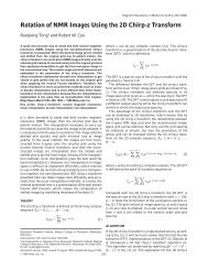
FIG. 2. Regressors for an epoch-related or block design (top) and 

an event-related design (bottom) with 128 scans and a TR of 1.7 s. 

Both sets of regressors were constructed by convolving the appropriate 

stimulus function (box-car for the block design and a stick function 

for the event-related design) and its temporal derivative with 

the canonical HRF depicted in Fig. 1. These regressors have been 

orthogonalized and Euclidean normalized.


199 

or potentially invalid (i.e., not robust). The position 

adopted in this paper is that, for fMRI data analysis, a 

minimum variance filter is not appropriate. Instead we 

would like to find a minimum bias filter. This is difficult 

because one needs to know how the serial correlations 

that are likely to be encountered deviate from the 

assumed form. The next subsection presents a way of 

estimating the expected bias and efficiency, given the 

probability distribution of the intrinsic correlations. 

Using empirical estimates of this distribution it is 

shown that suppressing both high and low frequencies 

with band-pass filtering is required to minimize bias. 

The expected values for bias and efficiency are then 

used to compare three filtering strategies, (i) whitening, 

(ii) high-pass, and (iii) band-pass (i.e., high pass 

with smoothing) filtering, under different models of the 

correlations. In brief it will be shown that supplementing 

high-pass filtering with smoothing has an important 

role in reducing bias whatever model is assumed. 

This section concludes by noting that minimizing bias 

over a range of deviations from the assumed form for 

the correlations also renders bias less sensitive to spatial 

variations in serial correlations from voxel to voxel. 

Efficiency and Bias 

Here we provide expressions for the efficiency and 

bias for any experimental design, embodied in the explanatory 

variables or regressors that comprise the 

design matrix X and any contrast or compound of parameter 

estimates specified with a vector of contrast 

weights. Consider the general linear model 

Sy SX SK i z, (1) 

where y isa(n 1) response variable (measured fMRI 

signal at any voxel) and S is an extrinsic or applied 

temporal filter matrix. If S has a Toeplitz form then it 

can be considered as an applied (de)convolution. However, 

generally S can take any form. A distinction is 

made between the true intrinsic correlations and those 

assumed. These correlations are characterized by the 

(n n) convolution matrices K i and K a , respectively, 

with an ensuing noise process K i z where z is an independent 

innovation (0, 2 I). 

The corresponding autocorrelation matrices are V i 

K i K i T and V a K a K a T . The general least-squares estimator 

of the parameters is 

ˆ GLS X T S T SX 1 SX T Sy SX Sy, (2) 

where 

denotes the pseudoinverse. The efficiency of 

estimating a particular contrast of parameters is inversely 

proportional to the contrast variance, 

varc T ˆ GLS 2 c T SX SV i S T SX T c, (3) 

where c is a vector of contrast weights. One might 

simply proceed by choosing S to maximize efficiency or, 

equivalently, minimize contrast variance (see “Minimum 

Variance Filters”). However, there is another 

important consideration here: any statistic used to 

make an inference about the significance of the contrast 

is a function of that contrast and an estimate of its 

variance. This second estimate depends upon an estimate 

of 2 and an estimate of the intrinsic correlations 

V i (i.e., V a ). The estimator of the contrast variance will 

be subject to bias if there is a mismatch between the 

assumed and the actual correlations. Such bias would 

invalidate the use of theoretical distributions, of test 

statistics derived from the contrast, used to control 

false-positive rates. 

Bias can be expressed in terms of the proportional 

difference between the true contrast variance and the 

expectation of its estimator (see Appendix B for details), 

BiasS, V i 

1 traceRSV iS T c T SX SV a S T SX T c 

traceRSV a S T c T SX SV i S T SX T c , (4) 

where R I SX(SX) is a residual-forming matrix. 

When bias is less than zero the estimated standard 

error is too small and the ensuing T or F statistic will 

be too large, leading to capricious inferences (i.e., false 

positives). When bias is greater than zero the inference 

will be too conservative (but still valid). In short if K i 

K a then bias will depend on S. IfK i K a then bias 

0 but efficiency still depends upon S. 

Minimum Variance Filters 

Conventional signal processing approaches and estimation 

theory dictate that whitening the data engenders 

the most efficient parameter estimation. This corresponds 

to filtering with a convolution matrix S that 

is the inverse of the intrinsic convolution matrix K i 

(where K i V 1/2 i ). The resulting parameter estimates 

are optimally efficient among all linear, unbiased estimators 

and correspond to the maximum likelihood estimators 

under Gaussian assumptions. More formally, 

the general least-squares estimators ˆ GLS are then 

equivalent to the Gauss–Markov or linear minimum 

variance estimators ˆ GM (Lawson and Hanson, 1974). 

In order to whiten the data one needs to know, or 

estimate, the intrinsic correlation structure. This reduces 

to finding an appropriate model for the autocorrelation 

function or spectral density of the error terms 

and then estimating the parameters of that model. 

Clearly one can never know the true structure but we 

can compare different models to characterize their relative 

strengths and weaknesses. In this paper we will 

take a high-order (16) autoregressive model as the


FIG. 3. Spectral densities (top) and corresponding autocorrelation 

functions (bottom) for the residual terms of a fMRI time series 

averaged over 512 voxels. Three cases are shown: (i) An AR(16) 

model estimated using the Yule–Walker method (this is taken to be 

a good approximation to the true correlations). The “bump” in the 

spectrum at around 1/32 Hz may reflect harmonics of random variations 

in trial-to-trial responses (every 16 s). (ii) An AR(1) model 

estimate using the same method. (iii) For a model of the form (q 1 /f 

q 2 ) where f is frequency in Hz. These data came from a single-subject, 

event-related, single-word-presentation fMRI study acquired with 

multislice EPI at 2 T with a TR of 1.7 s. The words were presented 

every 16 s. The data were globally normalized, and fitted eventrelated 

responses (Josephs et al., 1997) were removed. The 512 

voxels were selected on the basis of a nontrivial response to acoustic 

stimulation, based on the F ratio in a conventional SPM analysis 

(P 0.001 uncorrected). This ensured that the ensuing gray-matter 

voxels represented a fairly homogeneous population in terms of their 

functional specialization. 

“gold standard” and evaluate simpler, but commonly 

used, models in relation to it. In other words we will 

consider the AR(16) model as an approximation to the 

true underlying correlations. The problem of estimating 

serial correlations is highlighted in Fig. 3. Here the 

residuals from a long (512-scan, TR 1.7 s) time series 

were used to estimate the spectral density and associated 

autocorrelation functions (where one is the 

Fourier transform of the other) using the Yule–Walker 

method with an autoregression order of 16 (see Appendix 

A). The data came from a single-subject eventrelated 

study using sparse single-word presentations 

every 16 s. Evoked responses were removed following 

global normalization. Estimates of the autocorrelation 

functions and spectral densities using a commonly assumed 

AR(1) model (Bullmore et al., 1996) and a modified 

1/f model (Zarahn et al., 1997) are also shown. The 

AR(1) is inadequate in that it fails to model either 

long-range (i.e., low frequencies) or intermediate correlations. 

The modified 1/f model shown here is a good 

approximation for the short-range and intermediate 

correlations but fails to model the long-range correlations 

as well as it could. Any discrepancy between the 

assumed and the actual correlation structure means 

that, when the data are whitened in accord with the 

assumed models, the standard error of the contrast is 

biased. This leads directly to bias in the ensuing statistics. 

For example the T statistic is simply the quotient 

of the contrast and its estimated standard error. 

It should be noted that the simple models would fit 

much better if drifts were first removed from the time 

series. However, this drift removal corresponds to 

high-pass filtering and we want to make the point that 

filtering is essential for reducing the discrepancy between 

assumed and actual correlations (see below). 

This bias is illustrated in Fig. 4 under a variety of 

model-specific minimum-variance filters. Here the regressors 

from the epoch- and event-related designs in 

Fig. 2 were used as the design matrix X, to calculate 

the contrast variance and bias in the estimate of this 

variance according to Eq. (3) and Eq. (4), where 

V i V AR(16) , 

V a V i 

V AR(1) 

V 1/f 

1 

1 

i 

“correct” model 

1 

K 

, S K AR(1) AR1 model 

1 

. 

K 1/f 

1/f model 

1 “none” 

The variances in Fig. 4 have been normalized by the 

minimum variance possible (i.e., that of the “correct” 

model). The biases are expressed in terms of the proportion 

of variance incorrectly estimated. Obviously 

the AR(16) model gives maximum efficiency and no 

bias (bias 0) because we have used the AR(16) estimates 

as an approximation to the actual correlations. 

Any deviation from this “correct” form reduces efficiency 

and inflates the contrast variance. Note that 

misspecifying the form for the serial correlations has 

inflated the contrast variance more for the event-related 

design (bottom) relative to the epoch-related design 

(top). This is because the regressors in the epochrelated 

design correspond more closely to eigenvectors 

of the intrinsic autocorrelation matrix (see Worsley


201 

because a large number of scans enter into the estimation 

in fixed-effect analyses, and random-effects analyses 

(with fewer degrees of freedom) do not have to 

contend with serial correlations. 

FIG. 4. Efficiencies and biases computed according to Eq. (3) and 

Eq. (4) in the main text for the regressors in Fig. 2 and contrasts of 

[1 0] and [0 1] for three models of intrinsic correlations [AR(16), 

AR(1), and the modified 1/f models] and assuming they do not exist 

(“none”). The results are for the Gauss–Markov estimators (i.e., 

using a whitening strategy based on the appropriate model in each 

case) using the first model [AR(16)] as an approximation to the true 

correlations. The contrast variances have been normalized to the 

minimum attainable. The bias and increased contrast variance induced 

result from adopting a whitening strategy when there is a 

discrepancy between the actual and the assumed intrinsic correlations. 

and Friston, 1995). Generally if the regressors conform 

to these eigenvectors then there is no loss of efficiency. 

The bias incurred by mis-specification can be substantial, 

resulting in an over- [AR(1)] or under- (1/f and 

“none”) estimation of the contrast variance leading, in 

turn, to inexact tests using the associated T statistic 

that are unduly insensitive [AR(1)] or invalid (1/f and 

“none”). The effect is not trivial. For example the bias 

engendered by assuming an AR(1) form in Fig. 4 is 

about 24%. This would result in about a 10% reduction 

of T values and could have profound effects on inference. 

In summary the use of minimum variance, or maximum 

efficiency, filters can lead to invalid tests. This 

suggests that the use of whitening is inappropriate and 

the more important objective is to adopt filtering strategies 

that minimize bias to ensure that the tests are 

robust in the face of misspecified autocorrelation structures 

(i.e., their validity is retained). The minimum 

bias approach is even more tenable given that sensitivity 

in fMRI is not generally a great concern. This is 

Minimum Bias Filters 

There are two fundamental problems when trying to 

model intrinsic correlations: (i) one generally does not 

know the true intrinsic correlations and (ii) even if they 

were known for any given voxel time series, adopting 

the same assumptions for all voxels will lead to bias 

and loss of efficiency because each voxel has a different 

correlation structure (e.g., brain-stem voxels will be 

subject to pulsatile effects, ventricular voxels will be 

subject to CSF flow artifacts, white matter voxels will 

not be subject to neurogenic noise). It should be noted 

that very reasonable methods have been proposed for 

local estimates of spatially varying noise (e.g., Lange 

and Zeger, 1997). However, in this paper we assume 

that computational, and other, constraints require us 

to use the same statistical model for all voxels. 

One solution to the “bias problem” is described in 

Worsley and Friston (1995) and involves conditioning 

the serial correlations by smoothing. This effectively 

imposes a structure on the intrinsic correlations that 

renders the difference between the assumed and the 

actual correlations less severe. Although generally less 

efficient, the ensuing inferences are less biased and 

therefore more robust. The loss of efficiency can be 

minimized by appropriate experimental design and 

choosing a suitable filter S. In other words there are 

certain forms of temporal filtering for which SV i S T 

SV a S T even when V i is not known [see Eq. (4)]. These 

filters will minimize bias. The problem is to find a 

suitable form for S. 

One approach to designing a minimum bias filter is 

to treat the intrinsic correlation V i , not as an unknown 

deterministic variable, but as a random variable, 

whose distributional properties are known or can be 

estimated. We can then choose a filter that minimizes 

the expected square bias over all V i , 

S MB min arg S S 

S biasS, V i 2 pV i dV i . 

(5) 

Equation (5) says that the ideal filter would minimize 

the expected or mean square bias over all intrinsic 

correlation structures encountered. An expression for 

mean square bias and the equivalent mean contrast 

variance (i.e., 1/efficiency) is provided in Appendix C. 

This expression uses the first and second order moments 

of the intrinsic autocorrelation function, parameterized 

in terms of the underlying autoregression co-


might posit band-pass filtering as a minimum bias 

filter. In the limit of very narrow band-pass filtering 

the spectral densities of the assumed and actual correlations, 

after filtering, would be identical and bias 

would be negligible. Clearly this would be inefficient 

but suggests that some band-pass filter might be an 

appropriate choice. Although there is no single universal 

minimum bias filter, in the sense it will depend on 

the design matrix and contrasts employed and other 

data acquisition parameters; one indication of which 

frequencies can be usefully attenuated derives from 

examining how bias depends on the upper and lower 

cutoff frequencies of a band-pass filter. 

Figure 6 shows the mean square bias and mean 

contrast variance incurred by varying the upper and 

lower band-pass frequencies. These results are based 

on the epoch-related regressors in Fig. 2 and assume 

that the intrinsic correlations conform to the AR(16) 

estimate. This means that any bias is due to variation 

FIG. 5. Characterizing the variability in intrinsic correlations. 

Top: The 16 partial derivatives of the autocorrelation function with 

respect to the eigenvectors of the covariance matrix of the underlying 

autoregression coefficients. These represent changes to the autocorrelation 

function induced by the principal components of variation 

inherent in the coefficients. The covariances were evaluated over the 

voxels described in Fig. 2. Lower left: The associated eigenvalue 

spectrum. Lower right: The autocorrelation function associated with 

the mean of the autoregression coefficients. These characterizations 

enter into Eq. (C.3) in Appendix C, to estimate the mean square bias 

for a given filter. 

efficients. More precisely, given the expected 

coefficients and their covariances, a simple secondorder 

approximation to Eq. (5) obtains in terms of the 

eigenvectors and eigenvalues of the AR coefficient covariance 

matrix. These characterize the principal variations 

about the expected autocorrelation function. 

Empirical examples are shown in Fig. 5, based on the 

variation over gray matter voxels in the data used in 

Fig. 2. Here the principal variations, about the expected 

autocorrelation function (lower right), are presented 

(top) in terms of partial derivatives of the autocorrelation 

function with respect to the autoregressive 

eigenvectors (see Appendix C). 

The expressions for mean square bias and mean 

contrast variance will be used in the next subsection to 

evaluate the behavior of three filtering schemes in 

relation to each other and a number of different correlation 

models. First however, we will use them to motivate 

the use of band-pass filtering: Intuitively one 

FIG. 6. Top: Mean square bias (shown in image format in inset) 

as a function of high- and low-pass cutoff frequencies defining a 

band-pass filter. Darker areas correspond to lower bias. Note that 

minimum bias attains when a substantial degree of smoothing or 

low-pass filtering is used in conjunction with high-pass filtering 

(dark area on the middle left). Bottom: As for the top but now 

depicting efficiency. The gray scale is arbitrary.


203 

about that estimate and not due to specifying an inappropriately 

simple form for the correlations. 3 

The 

ranges of upper and lower band-pass frequencies were 

chosen to avoid encroaching on frequencies that contain 

signal. This ensured that efficiency was not severely 

compromised. The critical thing to note from 

Fig. 6 is that the effects of low-pass and high-pass 

filtering are not linearly separable. In other words 

low-pass filtering or smoothing engenders minimum 

bias but only in the context of high-pass filtering. It is 

apparent that the minimum bias obtains with the 

greatest degree of smoothing examined but only in 

conjunction with high-pass filtering, at around 1/96 per 

second. In short, band-pass filtering (as opposed to 

high- or low-pass filtering on their own) minimizes bias 

without a profound effect on efficiency. Interestingly, 

in this example, although increasing the degree of 

smoothing or low-pass filtering increases contrast variance 

(i.e., decreases efficiency), at high degrees of 

smoothing the minimum variance high-pass filter is 

very similar to the minimum bias filter (see Fig. 6). 

These results used filter matrices that have a simple 

form in frequency space but are computationally expensive 

to implement. Next we describe a band-pass 

filter used in practice (e.g., in SPM99) and for the 

remainder of this paper. 

Computationally Efficient Band-Pass Filters 

The filter S can be factorized into low- and highpass 

4 components S S L S H . The motivation for this is 

partly practical and speaks to the special problems of 

fMRI data analysis and the massive amount of data 

that have to be filtered. The implementation of the 

filter can be made computationally much more efficient 

if the high frequencies are removed by a sparse 

Toeplitz convolution matrix and the high-pass component 

is implemented by regressing out low-frequency 

components. In this paper we choose S L so that its 

transfer function corresponds to that of the hemodynamic 

response function (the implied kernel is, however, 

symmetrical and does not induce a delay). This is 

a principled choice because it is in these frequencies 

that the neurogenic signal resides. S H is, effectively, 

the residual-forming matrix associated with a discrete 

cosine transform set (DCT) of regressors R up to a 

frequency specified in term of a minimum period, expressed 

in seconds. In this paper we use a cutoff period 

3 An AR(16) model stands in here for nearly every other possible 

model of intrinsic correlations. For example an AR(16) model can 

emulate the AR plus white noise model of Purdon and Weisskoff 

(1998). 

4 The terms low- and high-pass filtering are technically imprecise 

because the linear filter matrices are not generally convolution matrices 

(i.e., S H does not have a Toeplitz form). However, they remove 

high- and low-frequency components, respectively. 

FIG. 7. The spectral density of a band-pass filter based on the 

hemodynamic response function in Fig. 1 (solid line) and a high-pass 

component with a cutoff at 1/64 Hz (broken line). The corresponding 

symmetrical filter kernels are shown in the inset for the high-pass 

filter (broken line) and band-pass filter (solid line). 

of 64 s. 5 Some people prefer the use of polynomial or 

spline models for drift removal because the DCT imposes 

a zero slope at the ends of the time series and this 

is not a plausible constraint. The (squared) transfer 

functions and kernels associated with the high-pass 

and combined high- and low-pass (i.e., band-pass) filters 

are shown in Fig. 7. 

The effect of filtering the data is to impose an autocorrelation 

structure or frequency profile on the error 

terms. This reduces the discrepancy between the underlying 

serial correlations and those assumed by any 

particular model. This effect is illustrated in Fig. 8 in 

which the band-pass filter in Fig. 7 has been applied to 

the empirical time series used above. Filtering markedly 

reduces the differences among the spectral density 

and autocorrelation estimates using the various models 

(compare Fig. 8 with Fig. 3). The question addressed 

in the next subsection is whether this filter 

reduces mean square bias and, if so, at what cost in 

terms of mean efficiency. 

An Evaluation of Different Filtering Strategies 

In this subsection we examine the effect of filtering 

on mean contrast variance (i.e., mean 1/efficiency) and 

mean square bias using the expressions in Appendix C. 

This is effected under three different models of serial 

5 In practice filtering is implemented as Sy S L S H y S L (y 

R(R T y)). This regression scheme eschews the need to actually form a 

large (nonsparse) residual-forming matrix associated with the DCT 

matrix R. This form for S can be implemented in a way that gives a 

broad range of frequency modulation for relatively small numbers of 

floating point operations. Note that R is a unit orthogonal matrix. R 

could comprise a Fourier basis set or indeed polynomials. We prefer 

a DCT set because of its high efficiency and its ability to remove 

monotonic trends.


where S s F (1 s)1; 1 is the identity matrix and 

s is varied between 0 (no filtering) and 1 (filtering with 

F). The models and filters considered correspond to 

V a V AR(1) 

V 1/f and F 

V AR(16) 

V a 1/2 “whitening” 

S H “high-pass” 

S L S H “band-pass” . 

Mean square bias and mean contrast variance are 

shown as functions of the filtering parameter s in Fig. 

9 for the various schema above. The effect on efficiency 

is remarkably consistent over the models assumed for 

the intrinsic correlations. The most efficient filter is a 

whitening filter that progressively decreases the expected 

contrast variance. High-pass filtering does not 

FIG. 8. The spectral density and autocorrelation functions predicted 

on the basis of the three models shown in Fig. 3, after filtering 

with the band-pass filter in Fig. 7. Compare these functions with 

those in Fig. 3. The differences are now ameliorated. 

correlations: (i) AR(1), (ii) 1/f, and (iii) AR(16). Again 

we will assume that the AR(16) estimates are a good 

approximation to the true intrinsic correlations. For 

each model we compared the effect of filtering the data 

with whitening. In order to demonstrate the interaction 

between high- and low-pass filtering we used a 

high-pass filter and a band-pass filter. The latter corresponds 

to high-pass filtering with smoothing. The 

addition of smoothing is the critical issue here: The 

high-pass component is motivated by considerations of 

both bias and efficiency. One might expect that highpass 

filtering would decrease bias by removing low 

frequencies that are poorly modeled by simple models. 

Furthermore the effect on efficiency will be small because 

the minimum variance filter is itself a high-pass 

filter. On the other hand smoothing is likely to reduce 

efficiency markedly and its application has to be justified 

much more carefully. 

The impact of filtering can be illustrated by parametrically 

varying the amount of filtering with a filter F, 

FIG. 9. The effect of filtering on mean square bias and mean 

contrast variance when applying three filters: the band-pass filter in 

Fig. 8 (solid lines), the high-pass filter in Fig. 8 (dashed lines), and a 

whitening filter appropriate to the model assumed for the intrinsic 

correlations (dot–dash lines). Each of these filters was applied under 

three models: an AR(1) model (top), a modified 1/f model (middle), 

and an AR(16) model (bottom). The expected square biases (left) and 

contrast variances (right) were computed as described in Appendix C 

and plotted against a parameter s that determines the degree of 

filtering applied (see main text).


205 

markedly change this mean contrast variance and renders 

the estimation only slightly less efficient than no 

filtering at all. The addition of smoothing to give bandpass 

filtering decreases efficiency by increasing the 

mean contrast variance by about 15%. The effects on 

mean square bias are similarly consistent. Whitening 

attenuates mean square bias slightly. High-pass filtering 

is more effective at attenuating bias but only for 

the AR(1) model. This is because the whitening filters 

for the 1/f and AR(16) models more closely approximate 

the high-pass filter. The addition of smoothing engenders 

a substantial and consistent reduction in bias, 

suggesting that, at least for the acquisition parameters 

implicit in these data, smoothing has an important role 

in minimizing bias. This is at the expense of reduced 

efficiency. 

The profiles at the bottom in Fig. 9 are interesting 

because, as in the analysis presented in Fig. 6, the 

mean intrinsic correlations and assumed autocorrelation 

structure are taken to be the same. This means 

that any effects on bias or efficiency are due solely to 

variations about that mean (i.e., the second term in Eq. 

(C.3), Appendix C). The implication is that even a sophisticated 

autocorrelation model will benefit, in terms 

of inferential bias, from the particular band-pass filtering 

considered here. 

Spatially Varying Intrinsic Correlations 

In the illustrative examples above we have assumed 

that the variation within one voxel, over realizations, 

can be approximated by the variation over realizations 

in different gray-matter voxels that show a degree of 

functional homogeneity. The second problem, introduced 

at the beginning of this section, is that even if we 

assume the correct form for one voxel then we will be 

necessarily incorrect for every other voxel in the brain. 

This reflects the spatially dependent nature of temporal 

autocorrelations (see also Locascio et al., 1997). 

Assuming the same form for all voxels is a special 

constraint under which analyses of fMRI data have to 

operate. This is because we would like to use the same 

statistical model for every voxel. There are both computational 

and theoretical reasons for this, which derive 

from the later use of Gaussian Field theory when 

making inferences that are corrected for the volume 

analyzed. The theoretical reasons are that different 

intrinsic correlations would lead to statistics with different 

(effective) degrees of freedom at each voxel. 

Whether Gaussian Field theory is robust to this effect 

remains to be addressed. 

Not only does appropriate temporal filtering reduce 

bias engendered by misspecification of the intrinsic 

correlations at any one voxel, and stochastic variations 

about that specification, but it also addresses the problem 

of spatially varying serial correlations over voxels. 

FIG. 10. The distribution of bias (top) and contrast variance 

(bottom) over voxels using an AR(16) model to estimate intrinsic 

correlations at 512 voxels and assuming the same AR(1) autocorrelation 

structure over voxels. Distributions are shown with band-pass 

filtering (open bars) and with whitening (filled bars). Note how 

band-pass filtering reduces bias (at the expense of reduced efficiency). 

Efficiency is proportional to the inverse of the contrast variance. 

The top of Fig. 10 shows bias, computed using Eq. (3) 

over 512 voxels using an AR(16) voxel-specific estimate 

for the intrinsic correlations V i and an AR(1) model 

averaged over all voxels for the assumed correlations 

V a . With whitening the biases (solid bars) range from 

50 to 250%. With band-pass filtering (open bars) they 

are reduced substantially. The effect on efficiency is 

shown at the bottom. Here filtering increases the contrast 

variance in a nontrivial way (by as much as 50% 

in some voxels). It is interesting to note that spatially 

dependent temporal autocorrelations render the efficiency 

very variable over voxels (by nearly an order of 

magnitude). This is important because it means that 

fMRI is not homogeneous in its sensitivity to evoked 

responses from voxel to voxel, simply because of differences 

in serial correlations.


DISCUSSION 

This paper has addressed temporal filtering in fMRI 

time-series analysis. Whitening serially correlated 

data is the most efficient approach to parameter estimation. 

However, whitening can render the analysis 

sensitive to inferential bias, if there is a discrepancy 

between the assumed and the actual autocorrelations. 

This bias, although not expressed in terms of the estimated 

model parameters, has profound effects on any 

statistic used for inference. The special constraints of 

fMRI analysis ensure that there will always be a misspecification 

of the intrinsic autocorrelations because 

of their spatially varying nature over voxels. One resolution 

of this problem is to filter the data to ensure 

bias is small while maintaining a reasonable degree of 

efficiency. 

Filtering can be chosen in a principled way to maintain 

efficiency while minimizing bias. Efficiency can be 

retained by band-pass filtering to preserve frequency 

components that correspond to signal (i.e., the frequencies 

of the HRF) while suppressing high- and lowfrequency 

components. By estimating the mean square 

bias over the range of intrinsic autocorrelation functions 

that are likely to be encountered, it can be shown 

that supplementing a high-pass filter with smoothing 

has an important role in reducing bias. 

The various strategies that can be adopted can be 

summarized in terms of two choices: (i) the assumed 

form for the intrinsic correlations V a and (ii) the filter 

applied to the data S. Permutations include 

1 1 

V a VAR(p) 

, 

V AR(p) 

1 

S L S H 

S 1 

S L S H 

K AR(p) 

ordinary least squares 

conventional “filtering” SPM97 

conventional “whitening” , 

band-pass filtering SPM99 

where the assumed form is an AR(p) model. The last 

strategy, adopted in SPM99, is motivated by a balance 

between efficiency and computational expediency. Because 

the assumed correlations V a do not enter explicitly 

into the computation of the parameter estimates 

but only into the subsequent estimation of their standard 

error (and ensuing T or F statistics), the autocorrelation 

structure and parameter estimation can be 

implemented in a single pass through the data. SPM99 

has the facility to use an AR(1) estimate of intrinsic 

correlations, in conjunction with (separately) specified 

high- and low-pass filtering. 

A further motivation for filtering the data, to exert 

some control over the variance–bias trade-off, is that 

the exact form of serial correlations will vary with 

scanner, acquisition parameters, and experiment. For 

example the relative contribution of aliased biorhythms 

will change with TR and field strength. By 

explicitly acknowledging a discrepancy between the 

assumed approximation to underlying correlations a 

consistent approach to data analysis can be adopted 

over a range of experimental parameters and acquisition 

systems. 

The issues considered in this paper apply even when 

the repetition time (TR) or interscan interval is long. 

This is because serial correlations can enter as lowfrequency 

components, which are characteristic of all 

fMRI time series, irrespective of the TR. Clearly as the 

TR gets longer, higher frequencies cease to be a consideration 

and the role of low-pass filtering or smoothing 

in reducing bias will be less relevant. 

The conclusions presented in this paper arise under 

the special constraints of estimating serial correlations 

in a linear framework and, more specifically, using 

estimators that can be applied to all voxels. The inherent 

trade-off between the efficiency of parameter estimation 

and bias in variance estimation is shaped by 

these constraints. Other approaches using, for example, 

nonlinear observation models, may provide more 

efficient and unbiased estimators than those we have 

considered. 

It should be noted that the main aim of this paper is 

to provide an analytical framework within which the 

effects of various filtering strategies on bias and efficiency 

can be evaluated. We have demonstrated the 

use of this framework using only one data set and do 

not anticipate that all the conclusions will necessarily 

generalize to other acquisition parameters or statistical 

models. What has been shown here is, however, 

sufficient to assert that, for short repetition times, 

band-pass filtering can have an important role in ameliorating 

inferential bias and consequently in ensuring 

the relative robustness of the resulting statistical tests. 

APPENDIX A 

Forms of Intrinsic and Assumed Autocorrelations 

A distinction is made between the true intrinsic autocorrelations 

in a fMRI time series of length n and 

those assumed. These correlations are characterized by 

the (n n) convolution matrices K i and K a , respectively, 

with an ensuing noise process K i z, where z, 

is an independent innovation (0, 2 I) and 

diag{K i K T i } 1. The corresponding autocorrelation matrices 

are V i K i K T T. 

i and V a K a K a In this appendix 

we describe some models of intrinsic autocorrelations, 

specifically pth order autoregressive models AR(p) 

[e.g., AR(1); Bullmore et al., 1996)] or those that derive 

from characterizations of noise autocovariance structures 

or equivalently their spectral density (Zarahn et 

al., 1997). For any process the spectral density g() and


207 

autocorrelation function (t) are related by the Fourier 

transform pair 

t FTg, g IFTt, 

where V Toeplitzt and K V 1/2 . 

(A.1) 

Here t [0,1,...,n 1] is the lag in scans with (0) 

1 and 2i (i [0,...,n 1]) denotes frequency. 

The Toeplitz operator returns a Toeplitz matrix (i.e., a 

matrix that is symmetrical about the leading diagonal). 

The transfer function associated with the linear 

filter K is l(), where g() l() 2 . 

Autoregressive Models 

Autoregressive models have the following form: 

A z N 1 A 1 z, 

giving K a 1 A 1 where A 

 

0 0 0 0 . . . 

a 1 0 0 0 

a 2 a 1 0 0 

a 3 a 2 a 1 0 

· · 

··· 

·. 

(A.2) 

The autoregression coefficients in the triangular matrix 

A can be estimated using 

a a 1 ,...,a p 

 

1 1 ··· p 

1 1 

· 

··· 

· 1 

··· 

· 

p ··· 1 1 

1 

1 

2 

p 

··· 

1. 

(A.3) 

The corresponding spectral density over n frequencies 

is given by 

g FT n 1, a 2 , 

(A.4) 

where FT n { }isan-point Fourier transform with zero 

padding (cf. the Yule–Walker method of spectral density 

estimation). With these relationships [(A.1) to 

(A.3)] one can take any empirical estimate of the autocorrelation 

function (t) and estimate the autoregression 

model-specific convolution K a and autocorrelation 

V a K a K a T matrices. 

Modified 1/f Models 

K a and V a can obviously be estimated using spectral 

density through Eq. (A.1) if the model of autocorrelations 

is expressed in frequency space; here we use the 

analytic form suggested by the work of Zarahn et al. 

(1997), 

s q 1 

q 2, where g s 2 . (A.5) 

Note that Eq. (A.5) is linear in the parameters which 

can therefore be estimated in an unbiased manner 

using ordinary least squares. 

APPENDIX B 

Efficiency and Bias 

In this section we provide expressions for the efficiency 

and bias for any design matrix X and any contrast 

of parameter estimates specified with a vector of 

contrast weights c (this framework serves all the filtering 

schemes outlined in the main text). These expressions 

are developed in the context of the general 

linear model and parametric statistical inference (Friston 

et al., 1995). The bias here is in terms of the 

estimated standard error associated with any ensuing 

statistic. Consider the general linear model, 

Sy SX SK i z, 

(B.1) 

where y is the response variable and S is an applied 

filter matrix. The efficiency of the general least squares 

contrast estimator c T ˆ GLS is inversely proportional to 

its variance, 

Efficiency Varc T ˆ GLS 1 

Varc T ˆ GLS 2 c T SX SV i S T SX T c, 

(B.2) 

where denotes the pseudoinverse. Efficiency is maximized 

with the Gauss–Markov estimator, when S 

K 1 

i if the latter were known. However, there is another 

important consideration: The variance of the contrast 

has to be estimated in order to provide for statistical 

inference. This estimator and its expectation are 

Vˆ arc T ˆ 

 

y T S T R T RSy 

traceRSV a S T c T SX SV a S T SX T c 

Vˆ arc T ˆ 

2 traceRSV i S T 

traceRSV a S T 

c T SX SV a S T SX T c, 

(B.3) 

where R I SX(SX) is a residual-forming matrix. 

Bias can be expressed in terms of the (normalized) 

difference between the actual and the expected contrast 

variance estimators,


BiasS, V i 

Varc T ˆ GLS Vˆ arc T ˆ GLS 

Varc T ˆ GLS 

1 traceRSV iS T c T SX SV a S T SX T c 

traceRSV a S T c T SX SV i S T SX T c . 

(B.4) 

The critical thing about Eq. (B.4) is that bias is reduced 

as S induces more correlations relative to V i . In other 

words there are certain forms of temporal filtering for 

which SV i S T SV a S T even if V i V a . In extreme cases 

this allows one to essentially ignore intrinsic correlations 

with temporal filtering (i.e., V a I) although this strategy 

may be inefficient. Generally bias becomes sensitive 

to discrepancies between the actual and the assumed 

correlations when no filtering is employed and exquisitely 

so when S is a deconvolution matrix (e.g., whitening 

under the wrong assumptions about V i ). 

APPENDIX C 

Mean Square Bias 

In Appendix B the expression for bias treated V i as a 

fixed deterministic variable. In this appendix we derive 

an approximation for the expected squared bias when 

V i is a random stochastic variable parameterized in 

terms of its AR coefficients a. Let 

fr, S BiasVa Qr, S 2 . 

(C.1) 

The operator V{a} returns the autocorrelation matrix 

given the underlying AR coefficients according to A.2. a 

are the expected coefficients and Q contains the eigenvectors 

of Cov{a} (a a ) (a a ) T such that 

r Q T a a f 

r 0 

r r T 

(C.2) 

and is a leading diagonal matrix of associated eigenvalues. 

Mean square bias is approximated with 

S fr, S r f0, S i 

i 

2 

2 f0, S 

. (C.3) 

r i 

2 

This follows from taking the expectation of the secondorder 

approximation of the Taylor expansion of Eq. (C.1) 

around r 0 and substituting the expectations in Eq. 

(C.2). Note that, apart from the second-order approximation, 

no distributional assumptions have been made 

about the intrinsic AR coefficients. If these coefficients 

had a multivariate Gaussian distribution then (C.3) 

would be exactly right. The first term in (C.3) reflects the 

mean square bias attributable to the deviation between 

the assumed and the expected autocorrelation function. 

The second term reflects the contribution to bias due to 

variation about that expectation. An equivalent expression 

for mean contrast estimate variance obtains by substituting 

Eq. (B.2) into Eq. (C.1). 

In this paper the expectation and covariances of the 

AR coefficients were determined empirically using 

multiple realizations over gray-matter voxels and an 

AR(16) model. The partial derivatives in C.3 were estimated 

numerically. 

ACKNOWLEDGMENTS 

K.J.F., O.J., and A.P.H., were funded by the Wellcome trust. We 

thank the two anonymous reviewers for guidance in the development 

and presentation of this work. 

REFERENCES 

Aguirre, G. K., Zarahn, E., and D’Esposito, M. 1997. Empirical analysis 

of BOLD fMRI statistics. II. Spatially smoothed data collected 

under the null hypothesis and experimental conditions. Neuro- 

Image 5: 199–212. 

Boynton, G. M., Engel, S. A., Glover, G. H., and Heeger, D. J. 1996. 

Linear systems analysis of functional magnetic resonance imaging 

in human V1. J. Neurosci. 16: 4207–4221. 

Bullmore, E. T., Brammer, M. J., Williams, S. C. R., Rabe-Hesketh, 

S., Janot, N., David, A., Mellers, J., Howard, R., and Sham, P. 

1996. Statistical methods of estimation and inference for functional 

MR images. Magn. Reson. Med. 35: 261–277. 

Friston, K. J., Jezzard, P. J., and Turner, R. 1994. Analysis of 

functional MRI time-series. Hum. Brain Mapp. 1: 153–171. 

Friston, K. J., Holmes, A. P., Worsley, K. J., Poline, J. B., Frith, C. D., 

and Frackowiak, R. S. J. 1995. Statistical parametric maps in 

functional imaging: A general linear approach. Hum. Brain Mapp. 

2: 189–210. 

Friston, K. J., Josephs, O., Rees, G., and Turner, R. 1998. Non-linear 

event-related responses in fMRI. Magn. Reson. Med. 39: 41–52. 

Holmes, A. P., Josephs, O., Büchel, C., and Friston, K. J. 1997. 

Statistical modelling of low frequency confounds in fMRI. Neuro- 

Image 5: S480. 

Josephs, O., Turner, R., and Friston, K. J. 1997. Event-related fMRI. 

Hum. Brain Mapp. 5: 243–248. 

Lange, N., and Zeger, S. 1997. Non-linear Fourier time series analysis 

for human brain mapping with functional MRI. Appl. Stats. 

46: 1–26. 

Lawson, C. L., and Hanson, R. J. 1974. Solving Least Squares Problems. 

Prentice Hall, New York. 

Locascio, J. J., Peggy, J., and Corkin, S. 1997. A method of adjusting 

for temporal and spatial correlations in analysis of mean fMRI 

signal intensity changes. NeuroImage 3: S76. 

Paradis, A.-L., Van de Morrtele, P.-F., Le Bihan, D., and Poline, J.-B. 

1998. Do high temporal frequencies of the event-related fMRI 

response have a more specific spatial localization. NeuroImage 

7: S606. 

Purdon, P. L., and Weisskoff, R. 1998. Effect of temporal autocorrelations 

due to physiological noise stimulus paradigm on voxel-level 

false positive rates in fMRI. Hum. Brain Mapp. 6: 239–249. 

Worsley, K. J., and Friston, K. J. 1995. Analysis of fMRI time-series 

revisited—Again. NeuroImage 2: 173–181. 

Zarahn, E., Aguirre, G. K., and D’Esposito, M. 1997. Empirical analyses 

of BOLD fMRI statistics. I. Spatially unsmoothed data collected 

under null-hypothesis conditions. NeuroImage 5: 179–197.

Bias and Efficiency in fMRI Time-Series Analysis - Purdue University

Create successful ePaper yourself

Delete template?

Save as template?