Linear Regression

Linear Regression
In this tutorial we will explore fitting linear regression models using STATA. We
will also cover ways of re-expressing variables in a data set if the conditions for
linear regression aren’t satisfied.
We will be working with the data set discussed in examples 9.43-44 on page 210
of the textbook. The data set consists of three variables waist (waist size in
inches), weight (weight in pounds) and fat (body fat in %) measured on 20 male
subjects. To access the data type:
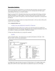
use http://www.stat.columbia.edu/~martin/W1111/Data/Body_fat
in the command window.
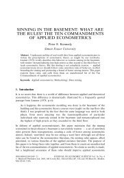
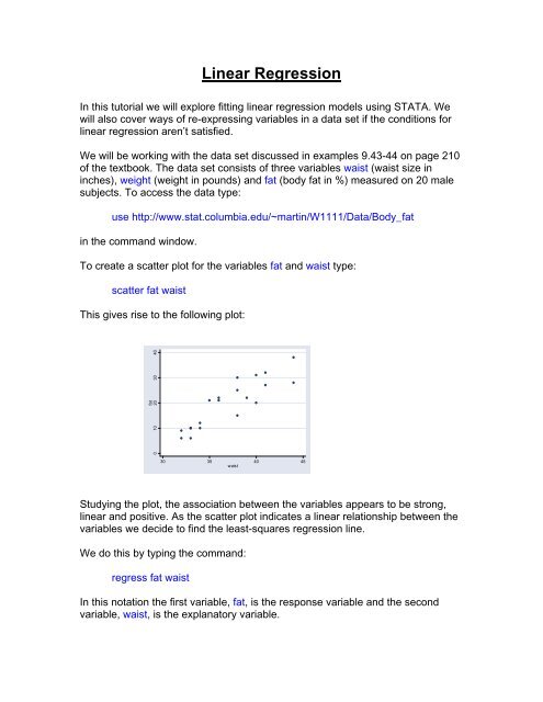
To create a scatter plot for the variables fat and waist type:
scatter fat waist
This gives rise to the following plot:
fat
0 10 20 30 40
30 35 40 45
waist
Studying the plot, the association between the variables appears to be strong,
linear and positive. As the scatter plot indicates a linear relationship between the
variables we decide to find the least-squares regression line.
We do this by typing the command:
regress fat waist
In this notation the first variable, fat, is the response variable and the second
variable, waist, is the explanatory variable.

This command gives rise to the following output in the results window:
The output indicates that the least-square regression line is given by.
fat
ˆ = −62.55
+ 2. 22waist
This implies that for each additional inch in waist size, the model predicts an
increase of 2.22% body fat. The fraction of the variability in fat that is explained
by the least squares line of fat on waist is equal to 0.7865.
Next, we want to calculate the predicted values from the regression. We can do
this by typing:
predict yhat, xb
This command is solely used to create a new variable, yhat, and there will be no
output in the results window. However, if you look in the variables window a new
variable yhat is now present. To plot the regression line together with the data
type:
scatter fat waist || line yhat waist
A vertical line can be obtained by simultaneously pressing the shift and the
backslash (\) button on your keyboard. This button is located directly above the
enter key. To obtain two vertical lines, repeat this procedure twice.

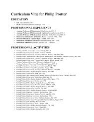
The command above tells STATA to create a scatterplot of fat against waist and
superimpose the line given by yhat created in the previous command. This
command gives the following plot:
fat/Linear prediction
0 10 20 30 40
30 35 40 45
waist
fat
Linear prediction
The line appears to fit the data well. However, it is important to make residual
plots when performing regression. We can calculate the residuals by typing the
command:
predict r, resid
Again, note that other than creating a new variable, r, there will be no additional
output. The new variable consists of the set of residuals, and a residual plot can
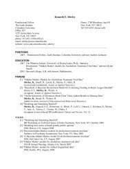
be created by typing:
scatter r waist
This gives rise to the following plot:
Residuals
-10 -5 0 5 10
30 35 40 45
waist
The residual plot shows no apparent pattern. The residual plot and the relatively
2
high value of R indicate that the linear model we fit is appropriate.

Re-expressing Data
Often the conditions necessary for performing linear regression aren’t satisfied in
a data set. However, it may still be possible to use these methods if we reexpress
one or both of the variables.
To re-express data we need be able to create new variables using STATA. We
can do this using the generate command. For example to create a new variable
named logx which is the logarithm of an already existing variable x, we type:
generate logx = log(x)
If we instead wanted to create a variable that is the square root of x, we could
type
generate sqx = sqrt(x)
In general, the command is on the format:
generate new_variable = expression(old_variable)
where expression is the mathematical function applied to the old variable.
Note that by default STATA uses log base e.
Linear regression using re-expressed data
In this portion of the tutorial we will be working with the data set discussed in
example 10.11 on page 256 of the textbook. The data set gives information on
the highest paid baseball players in the period spanning 1980-2001. The data set
consists of 3 variables player, year and salary. To access the data type:
use http://www.stat.columbia.edu/~martin/W1111/Data/salary
in the command window.
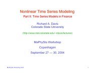
We begin by making a scatter plot of salary and year.
scatter salary year

This gives rise to the following plot:
salary
0 5 10 15 20 25
1980 1985 1990 1995 2000
year
The relationship between year and highest salary is moderately strong, positive
and curved. Since the scatter plot shows a curved relationship, a linear model is
not appropriate. However, it appears that taking the logarithm of salary may help
straighten the plot. We can generate a new variable named logsalary, which is
the logarithm of the variable salary, by typing:
generate logsalary = log(salary)
We can make a scatter plot of this new variable against year by typing
scatter logsalary year
This gives rise to the following plot:
logsalary
0 1 2 3
1980 1985 1990 1995 2000
year
It appears that the transformation has significantly straightened the scatter plot.
We can now proceed with fitting a linear regression model to the transformed
data by typing:
regress logsalary year
Note that now the response variable is logsalary instead of salary.

This gives rise to the following output:
The output indicates that the least-square regression line is given by.
log( salary
ˆ ) = −261.28
+ 0. 13year
The fraction of the variability in log(salary) that is explained by the least squares
line of log(salary) on year is equal to 0.9622.
Next, we want to calculate the predicted values from our regression. We can do
this by typing:
predict yhat, xb
Note that other than creating a new variable, yhat, there will be no additional
output. To plot the regression line together with the data type:
scatter logsalary year || line yhat year
The command above tells STATA to create a scatterplot of logsalary against year
and to superimpose the line given by yhat. This command gives the following
output
logsalary/Linear prediction
0 1 2 3
1980 1985 1990 1995 2000
year
logsalary
Linear prediction

The line appears to fit the data well. However, we always want to make sure to
check the residual plots. We can calculate the residuals by typing the command:
predict r, resid
Again, note that other than creating a new variable named r there will be no
additional output. We can use this new variable to create a residual plot by
typing:
scatter r year
This gives rise to the following output:
Residuals
-.4 -.2 -5.55e-17 .2 .4
1980 1985 1990 1995 2000
year
The residual plot shows no apparent pattern.
Homework:
Do problems RII.8 and 10.9 from the textbook.
Solve both of these problems using STATA. For each questions make sure to
hand in
(a) your log file,
(b) a scatter plot with a regression line superimposed,
(c) a residual plot, and
(d) answers to all the questions in the text.