An Asymptotic Theory for Weighted Least-Squares with Weights ...
An Asymptotic Theory for Weighted Least-Squares with Weights ...
An Asymptotic Theory for Weighted Least-Squares with Weights ...

Create successful ePaper yourself
Turn your PDF publications into a flip-book with our unique Google optimized e-Paper software.
<strong>An</strong> <strong>Asymptotic</strong> <strong>Theory</strong> <strong>for</strong> <strong>Weighted</strong> <strong>Least</strong>-<strong>Squares</strong> <strong>with</strong> <strong>Weights</strong> Estimated by<br />
Replication<br />
Raymond J. Carroll; Daren B. H. Cline<br />
Biometrika, Vol. 75, No. 1. (Mar., 1988), pp. 35-43.<br />
Stable URL:<br />
http://links.jstor.org/sici?sici=0006-3444%28198803%2975%3A1%3C35%3AAATFWL%3E2.0.CO%3B2-S<br />
Biometrika is currently published by Biometrika Trust.<br />
Your use of the JSTOR archive indicates your acceptance of JSTOR's Terms and Conditions of Use, available at<br />
http://www.jstor.org/about/terms.html. JSTOR's Terms and Conditions of Use provides, in part, that unless you have obtained<br />
prior permission, you may not download an entire issue of a journal or multiple copies of articles, and you may use content in<br />
the JSTOR archive only <strong>for</strong> your personal, non-commercial use.<br />
Please contact the publisher regarding any further use of this work. Publisher contact in<strong>for</strong>mation may be obtained at<br />
http://www.jstor.org/journals/bio.html.<br />
Each copy of any part of a JSTOR transmission must contain the same copyright notice that appears on the screen or printed<br />
page of such transmission.<br />
JSTOR is an independent not-<strong>for</strong>-profit organization dedicated to and preserving a digital archive of scholarly journals. For<br />
more in<strong>for</strong>mation regarding JSTOR, please contact support@jstor.org.<br />
http://www.jstor.org<br />
Wed Mar 28 11:53:08 2007
Biometrika (1988), 75, 1, pp. 35-43 <br />
Printed in Great Britain <br />
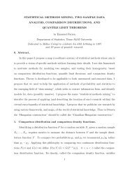
<strong>An</strong> asymptotic theory <strong>for</strong> weighted least-squares <strong>with</strong> weights<br />
estimated by replication<br />
BY RAYMOND J. CARROLL AND DAREN B. H. CLINE <br />
Department of Statistics, Texas A&M University, College Station, Texas 77843, U.S.A. <br />
SUMMARY<br />
We consider a heteroscedastic linear regression model <strong>with</strong> replication. To estimate<br />
the variances, one can use the sample variances or the sample average squared errors<br />
from a regression fit. We study the large-sample properties of these weighted least-squares<br />
estimates <strong>with</strong> estimated weights when the number of replicates is small. The estimates<br />
are generally inconsistent <strong>for</strong> asymmetrically distributed data. If sample variances are<br />
used based on m replicates, the weighted least-squares estimates are inconsistent <strong>for</strong><br />
m = 2 replicates even when the data are normally distributed. With between 3 and 5<br />
replicates, the rates of convergence are slower than the usual square root of N. With<br />
m>6 replicates, the effect of estimating the weights is to increase variances by<br />
(m -5)/(m -3), relative to weighted least-squares estimates <strong>with</strong> known weights.<br />
Some key words: Generalized least-squares; Heteroscedasticity; Regression; Replication.<br />
Consider a heteroscedastic linear regression model <strong>with</strong> replication:<br />
y..=xTp+~~~~<br />
r~<br />
(i=l,..., N;j=l, ...,m). (1.1)<br />
Here j? is a vector <strong>with</strong> p-components, and the E~ are independent and identically<br />
distributed random variables <strong>with</strong> mean zero and variance one. The heteroscedasticity<br />
in the model is governed by the unknown ai. We have taken the number of replicates at<br />
each xi to be the constant m primarily as a matter of convenience. In practice, it is fairly<br />
common that the number of design vectors N is large while the number of replicates m<br />
is small. Our intention is to construct an asymptotic theory in this situation <strong>for</strong> weighted<br />
least-squares estimates <strong>with</strong> estimated weights.<br />
As a benchmark, let iwLs be the weighted least-squares estimate <strong>with</strong> weights l/a:.<br />
Of course, since the ai are unknown this estimate cannot be calculated from data. If m<br />
is fixed and<br />
then<br />
N <br />
SwLs=plim N-' zxixT/ a:,<br />
N-oo i=l<br />
(N~)~(~WLS -P) + N(O, S&S).<br />
(1.2)<br />
One common method <strong>for</strong> estimating weights uses the inverses of the sample variances,<br />
The resulting weighted least-squares estimator will be denoted by bsv.
This method is particularly convenient because it involves sending only the estimated<br />
weights to a computer program <strong>with</strong> a weighting option. The obvious question is whether<br />
is,is any good, and whether the inferences made by the computer program have any<br />
reliability. In 00 3 and 4, we answer both questions in the negative, at least <strong>for</strong> normally<br />
distributed data <strong>with</strong> less than 10 replicates at each x. In many applied fields this is<br />
already folklore (Garden, Mitchell & Mills, 1980). Yates & Cochran (1938) have a nice<br />
discussion of the problems <strong>with</strong> using the sample variances to estimate the weights.<br />
More precisely, <strong>for</strong> normally distributed data we are able to describe the asymptotic<br />
distribution of bSV<strong>for</strong> every m. For m >:, this is an easy moment calculation and<br />
we show that psv is more variable than PwLsby a factor (m-3)/(m -5). The same<br />
result was obtained by Cochran (1937) <strong>for</strong> the weighted mean. Not only is fisv inefficient,<br />
but if one uses an ordinary weighted regression package to compute fisv, the standard<br />
errors from the package will be too small by a factor exceeding 20% unless m 2 10. For<br />
example, if one uses m =6 replicates, the efficiency <strong>with</strong> respect to weighted least-squares<br />
<strong>with</strong> known weights is only f, and all estimated standard errors should be multiplied by<br />
J3 = 1.732. For m
<strong>Weighted</strong> least-squares <strong>with</strong> weights estimated by replication 3 7<br />
These methods have been discussed in the literature <strong>for</strong> normally distributed errors.<br />
Bement & Williams (1969) use (1.3), and construct approximations, as m -, oo, <strong>for</strong> the<br />
exact covariance matrix of the resulting weighted least-squares estimate. They do not<br />
discuss asymptotic distributions as N -, oo <strong>with</strong> m fixed. Fuller & Rao (1978) use (1.4)<br />
while Cochran (1937) and Neyman & Scott (1948) use (1.5). Both find limiting distributions<br />
as N-, oo <strong>for</strong> fixed m 23, although the latter two papers consider only the case<br />
that xTp = p.<br />
One striking result concerns consistency. The estimates j,,, bELand jML are always<br />
consistent <strong>for</strong> symmetrically distributed errors but ge;erally<br />
n2t otherwise: see Theorems<br />
1 and 3. In O 5, we compute the limit distributions of PELand PML.The relative efficiency<br />
of the two is contrasted in the normal case <strong>for</strong> m 2 3, as follows.<br />
Remark 1. If ordinary least-squares isjess than 3 times more variable than weighted<br />
least-squares <strong>with</strong> known weights, then PELis more efficient than maximum likelihood.<br />
Remark 2. If ordinary least-squares is more than 5 times more variable than weighted<br />
least-squares <strong>with</strong> known weights, then maximum likelihood is more efficient.<br />
Further, <strong>for</strong> normally distributed data, maximum likelihood is more variable than<br />
weighted least-squares <strong>with</strong> known weights by a factor m/(m-2). This means a tripling<br />
of variance <strong>for</strong> m = 3 even when using maximum likelihood.<br />
2. ASSUMPTIONS AND CANONICAL DECOMPOSITION<br />
We will assume throughout that (xi, a,) are independent and identically distributed<br />
bounded random vectors, distributed independently of the {eij).We define zi = xi/ui and<br />
di= &,/ai. For any weighted least-squares estimator <strong>with</strong> estimated weights Gi = I/#,<br />
Assuming they exist, we note that the asymptotic covariance of the weighted and<br />
unweighted least-squares estimators are, respectively,<br />
3. WEIGHTINGWITH SAMPLE VARIANCES<br />
In this section, we describe consistency and asymptotic normality <strong>for</strong> weighted leastsquares<br />
estimates @, <strong>with</strong> the weights being the inverse of sample variances. We first<br />
describe the general case assuming that sufficient moments exist. We then look more<br />
closely at the case of normally distributed observations. In this set-up,<br />
Define qjk = E(~{ld*:~)and q k = E( JE~(J/~~~).<br />
The first result indicates that we obtain consistency only when<br />
qll= E (~~/ht) = 0.<br />
This is true <strong>for</strong> symmetrically distributed data, but generally not otherwise.
THEOREM1. (a) If v,, 0. Define p,(t) =<br />
E{wI(w s t)) and p2(t)= E{(UW)~I(UWS t)). Let (c,,, c2,) be constants satisfying, as<br />
Njoo, NPI(CIN)/CIN~ 1 and NP~(c~N)/c:N+1.<br />
If a,< 1, then S,= Sl(a,) will denote a positive stable random variable <strong>with</strong> Laplace<br />
trans<strong>for</strong>m E{exp (-tS,)) = exp {-I'(2 - a,)t"l/a,). If a, = 1 then S, = 1 almost surely. We
<strong>Weighted</strong> least-squares <strong>with</strong> weights estimated by replication 39<br />
denote by S2= S2(a2)a symmetric stable random variable <strong>with</strong> characteristic function<br />
E {exp (its,)) =exp [-r(3 - a,) cos ($~a,)(t(~2/{a~(l - a2))].<br />
Of course, if a, =2 then S, is standard normal.<br />
THEOREM2. Assume that p1E ~v(1-a,), p, E ~ v(2- a,) and that<br />
is asymptotically distributed as (Sl(al),S2(a2)).Suppose that, <strong>for</strong> some 6 >0 and all i, j,<br />
E ((z,IY)< <strong>for</strong> y =min (2, max (2a1,a,) +6). Then there exists Y2E RP, Y1p x ppositivedejinite,<br />
such that<br />
is asymptotically distributed as Y;' Y2. Further, <strong>for</strong> any b E R P, bTY1b and bTY2 have the<br />
same distributions, respectively, as<br />
Proof: Consider first the case a,< 1. From Theorem 1 of Cline (1988) we get<br />
is asymptotically distributed as ( Y,, Y,). In the case that a, = 1, then S1= 1 almost surely<br />
by Feller (1971, p. 236). From unpublished work of D. B. H. Cline and from Gnedenko<br />
& Kolmogorov (1954, p. 134), <strong>for</strong> each (j, k),<br />
plim c;A<br />
N<br />
i=l<br />
zijzikwi= E (z,zik).<br />
The convergence of the remaining terms, c& X ziuiwi,again follows from Theorem 1 of<br />
Cline (1988).<br />
In either case, convergence of the ratio bN follows. The limiting joint distribution is<br />
difficult to describe, but the stated marginal distributions of bTy1band bTy2can be<br />
inferred from Proposition 3 of Breiman (1965) and Theorem 3 of Maller (1981). One<br />
may also conclude that Y1 and Y2 are independent if a, = 1, since then Y1 is degenerate.<br />
Also, Y1 and Y, are independent if a, =2, since then Y, is Gaussian, and <strong>for</strong> such limits<br />
the non-Gaussian stable component is always independent of the Gaussian component<br />
(Sharpe, 1969).<br />
Note that, in Theorem 2, Y, and Y2 are not necessarily independent unless a, = 1 or<br />
a, =2. In the <strong>for</strong>mer case, Y1=E(zzT) almost surely, while in the latter case Y, is<br />
normally distributed <strong>with</strong> mean zero and covariance E(zzT).<br />
These are the following special cases.<br />
If (t/~,)~lpr (w > t) + 1 <strong>for</strong> y, >0, then we have the following:<br />
(i) if y1< 1, then a, = yl , clN =al {N/(l- al))l'nl, and S1is positive stable;<br />
(ii) if yl=l, then al=l, C1~=alN10gN,andS1=l;<br />
(iii) if yl>l, then al=l, clN=NE(w),and S1=l.
If (tla,) Y2 pr (1uwl > t) + 1 <strong>for</strong> y2>0, then we have the following:<br />
(i) if y,
<strong>Weighted</strong> least-squares <strong>with</strong> weights estimated by replication 41<br />
For each c, > 0, there exists c2> 0 such that<br />
and such that<br />
In addition, we assume the finite existence of<br />
77jk = E{E{/dfk(~)),Vlk = E{lEil'/dfk(~))
covariance Sit.Comparing PIEL <strong>with</strong> the maximum likelihood estimate PIML depends on<br />
how much bigger S,' is than S&. Detailed calculations verify Remarks 1 and 2 of § 1.<br />
Thus, doing iterative weighted least-squares may actually hurt, unless the starting value<br />
PIL is sufficiently bad.<br />
Our results can be summarized as follows.<br />
(i) If nothing is known about the structure of the sample variances, then none of the<br />
common weighted estimates can be assumed to be consistent <strong>for</strong> data from an asymmetric<br />
distribution.<br />
(ii) Using sample variances as a basis <strong>for</strong> estimating weights is inefficient unless the<br />
number of replicates m is fairly large, e.g. m 3 10.<br />
(iii) Using sample average squared errors from a preliminary fit to the regression<br />
function as a basis <strong>for</strong> estimating weights is typically more efficient than using sample<br />
variances. However, even here a fair number of replicates is helpful. For example, the<br />
maximum likelihood estimate <strong>for</strong> normally distributed data based on 6 replicates still<br />
has standard errors approximately 20% larger than ordinary weighted least-squares theory<br />
would suggest.<br />
There are at least two other methods <strong>for</strong> estimating the weights. The first is to model<br />
the variances parametrically, <strong>for</strong> example a,= a(xT~)~ (Carroll & Ruppert, 1987;<br />
Davidian & Carroll, 1987). The second is to per<strong>for</strong>m a nonparametric regression of (1.3)<br />
and (1.4) against the predictors and use this regression to estimate the weights (Carroll,<br />
1982).<br />
ACKNOWLEDGEMENT<br />
The work of R. J. Carroll was supported by the Air Force Office of Scientific Research.<br />
BEMENT, T. R. & WILLIAMS, J. S. (1969).Variance of weighted regression estimators when sampling errors<br />
are independent and heteroscedastic. J. Am. Statist. Assoc. 64, 1369-82.<br />
BREIMAN, L. (1965). On some limit theorems similar to the arc-sine law. <strong>Theory</strong> Prob. Applic. 10, 323-31.<br />
CARROLL, R. J. (1982). Adapting <strong>for</strong> heteroscedasticity in linear models. <strong>An</strong>n. Statist. 10, 1224-33.<br />
CARROLL, R. J. & RUPPERT, D. (1987). Trans<strong>for</strong>mations and Weighting in Regression. London: Chapman<br />
& Hall.<br />
CLINE, D. B. H. (1988). Joint stable attraction of two sums of products. J. Mult. <strong>An</strong>al. To appear.<br />
COCHRAN, W. G. (1937). Problems arising in the analysis of a series of similar experiments. J. R. Statist.<br />
SOC., SUPPI. 4, 102-18.<br />
DAVIDIAN, M. & CARROLL, R. J. (1987).Variance function estimation. J. Am. Statist. Assoc. 82. To appear.<br />
FELLER, W. (1971). <strong>An</strong> Introduction to Probability <strong>Theory</strong> and its Applications, 2. New York: Wiley.<br />
FULLER, W. A. & RAO, J. N. K. (1978). Estimation <strong>for</strong> a linear regression model <strong>with</strong> unknown diagonal<br />
covariance matrix. <strong>An</strong>n. Statist. 6, 1149-58<br />
GARDEN, J. S., MITCHELL, D. G. & MILLS, W. N. (1980). Nonconstant variance regression techniques <strong>for</strong><br />
calibration curve based analysis. <strong>An</strong>alytical Chemistry 52, 2310-5.<br />
GNEDENKO, B. V. & KOLMOGOROV,A. N. (1954). Limit Distributions <strong>for</strong> Sums of Independent Random<br />
Variables. Cambridge, Mass: Addison-Wesley.
<strong>Weighted</strong> least-squares <strong>with</strong> weights estimated by replication<br />
MALLER, R. A. (1981). A theorem on products of random variables, <strong>with</strong> applications to regression. Aust.<br />
J. Statist. 23, 177-85.<br />
NEYMAN,J. & SCOTT, E. L. (1948). Consistent estimators based on partially consistent observations.<br />
Econometrica 16, 1-32.<br />
SHARPE, M. (1969). Operator stable distributions on vector spaces. Trans. Am. Math. Soc. 136, 51-65.<br />
YATES,F. & COCHRAN,W. G. (1938). The analysis of groups of experiments. J. Agric. Sci. 28, 556-80.<br />
Reprinted (1970) in Experimental Design: Selected Papers of Frank Yates, pp. 121-45. London: Griffin.<br />
[Received May 1987. Revised September 19871<br />
43