1 An overview of almost sure convergence 2 Strong consistency of ...
1 An overview of almost sure convergence 2 Strong consistency of ...
1 An overview of almost sure convergence 2 Strong consistency of ...

Create successful ePaper yourself
Turn your PDF publications into a flip-book with our unique Google optimized e-Paper software.
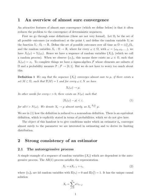
1 <strong>An</strong> <strong>overview</strong> <strong>of</strong> <strong>almost</strong> <strong>sure</strong> <strong>convergence</strong><br />
<strong>An</strong> attractive features <strong>of</strong> <strong>almost</strong> <strong>sure</strong> <strong>convergence</strong> (which we define below) is that it <strong>of</strong>ten<br />
reduces the problem to the <strong>convergence</strong> <strong>of</strong> deterministic sequences.<br />
First we go through some definitions (these are not very formal). Let Ω t be the set <strong>of</strong><br />
all possible outcomes (or realisations) at the point t, and define the random variable Y t as<br />
the function Y t : Ω t → R. Define the set <strong>of</strong> possible outcomes over all time as Ω = ⊗ ∞ t=1Ω t ,<br />
and the random variables X t : Ω → R, where for every ω ∈ Ω, with ω = (ω 0 ,ω 2 ,...), we<br />
have X t (ω) = Y t (ω t ). Hence we have a sequence <strong>of</strong> random variables {X t } t (which we call<br />
a random process). When we observe {x t } t , this means there exists an ω ∈ Ω, such that<br />
X t (ω) = x t . To complete things we have a sigma-algebra F whose elements are subsets <strong>of</strong><br />
Ω and a probability mea<strong>sure</strong> P : F → [0, 1]. But we do not have to worry too much about<br />
this.<br />
Definition 1 We say that the sequence {X t } converges <strong>almost</strong> <strong>sure</strong> to µ, if there exists a<br />
set M ⊂ Ω, such that P(M) = 1 and for every ω ∈ N we have<br />
X t (ω) → µ.<br />
In other words for every ε > 0, there exists an N(ω) such that<br />
|X t (ω) − µ| < ε, (1)<br />
for all t > N(ω). We denote X t → µ <strong>almost</strong> <strong>sure</strong>ly, as X t<br />
a.s.<br />
→ µ.<br />
We see in (1) how the definition is reduced to a nonrandom definition. There is an equivalent<br />
definition, which is explicitly stated in terms <strong>of</strong> probabilities, which we do not give here.<br />
The object <strong>of</strong> this handout is to give conditions under which an estimator â n converges<br />
<strong>almost</strong> <strong>sure</strong>ly to the parameter we are interested in estimating and to derive its limiting<br />
distribution.<br />
2 <strong>Strong</strong> <strong>consistency</strong> <strong>of</strong> an estimator<br />
2.1 The autoregressive process<br />
A simple example <strong>of</strong> a sequence <strong>of</strong> random variables {X t } which are dependent is the autogressive<br />
process. The AR(1) process satisfies the representation<br />
X t = aX t−1 + ǫ t , (2)<br />
where {ǫ t } t are iid random variables with E(ǫ t ) = 0 and E(ǫ 2 t) = 1. It has the unique causal<br />
solution<br />
∞∑<br />
X t = a j ǫ t−j .<br />
j=0<br />
1
From the above we see that E(X 2 t ) = (1 − a 2 ) −1 . Let σ 2 := E(X 2 0) = (1 − a 2 ) −1 .<br />
Question What can we say about the limit <strong>of</strong><br />
ˆσ 2 n = 1 n<br />
n∑<br />
Xt 2 .<br />
j=1<br />
• If E(ε 4 t) < ∞, then we show that E(ˆσ n − σ 2 ) 2 → 0 (Exercise).<br />
• What can we say about <strong>almost</strong> <strong>sure</strong> <strong>convergence</strong>?<br />
2.2 The strong law <strong>of</strong> large numbers<br />
Recall the strong law <strong>of</strong> large numbers; Suppose {X t } t is an iid sequence, and E(|X 0 |) < ∞<br />
then by the SLLN we have that<br />
1<br />
n<br />
n∑<br />
j=1<br />
X t<br />
a.s.<br />
→ E(X 0 ),<br />
for the pro<strong>of</strong> see Grimmet and Stirzaker (1994).<br />
• What happens when the random variables {X t } are dependent?<br />
• In this case we use the notion <strong>of</strong> ergodicity to obtain a similar result.<br />
2.3 Some ergodic tools<br />
Suppose {Y t } is an ergodic sequence <strong>of</strong> random variables (which implies that {Y t } t are identically<br />
distributed random variables). For the definition <strong>of</strong> ergodicity and a full treatment<br />
see, for example, Billingsley (1965).<br />
• A simple example <strong>of</strong> an ergodic sequence is {Z t }, where {Z t } t are iid random variables.<br />
Theorem 1 One variation <strong>of</strong> the ergodic theorem: If {Y t } is an ergodic sequence, where<br />
E(|g(Y t )|) < ∞. Then we have<br />
1<br />
n<br />
n∑<br />
i=1<br />
g(Y t ) a.s. → E(g(Y 0 )).<br />
We give some sufficient conditions for a process to be ergodic. The theorem below is a<br />
simplified version <strong>of</strong> Stout (1974), Theorem 3.5.8.<br />
Theorem 2 Suppose {Z t } is an ergodic sequence (for example iid random variables) and<br />
g : R ∞ → R is a continuous function. Then the sequence {Y t } t , where<br />
is an ergodic process.<br />
Y t = g(Z t ,Z t−1 ,...,),<br />
2
3<br />
(i) Example I Let us consider the sequence {X t }, which satisfies the AR(1) representation.<br />
We will show by using Theorem 2, that {X t } is an ergodic process. We know<br />
that X t has the unique (casual) solution<br />
X t =<br />
∞∑<br />
a j ǫ t−j .<br />
j=0<br />
The solution motivates us to define the function<br />
∞∑<br />
g(x 0 ,x 1 ,...) = a j x j .<br />
j=0<br />
We have that<br />
∞∑<br />
∞∑<br />
|g(x 0 ,x 1 ,...) − g(y 0 ,y 1 ,...)| = | a j x j − a j y j |<br />
≤<br />
j=0<br />
j=0<br />
∞∑<br />
a j |x j − y j |.<br />
j=0<br />
Therefore if max j |x j − y j | ≤ |1 − a|ε, then |g(x 1 ,x 2 ,...) − g(y 1 ,y 2 ,...)| ≤ ε. Hence<br />
the function g is continuous (under the sup-norm), which implies, by using Theorem<br />
2, that {X t } is an ergodic process.<br />
Application Using the ergodic theorem we have that<br />
1<br />
n<br />
n∑<br />
t=1<br />
X 2 t<br />
a.s.<br />
→ σ 2 .<br />
(ii) Example II A stochastic process <strong>of</strong>ten used in finance is the ARCH process. {X t } is<br />
said to be an ARCH(1) process if it satisfies the representation<br />
X t = σ t Z t<br />
σ 2 t = a 0 + a 1 X 2 t−1.<br />
It has <strong>almost</strong> <strong>sure</strong>ly the solution<br />
X 2 t = a 0<br />
∞<br />
∑<br />
j∏<br />
a j 1 Zt−i.<br />
2<br />
j=0 i=0<br />
Using the arguments above we can show that {X 2 t } t is an ergodic process.<br />
3 Likelihood estimation<br />
Our object here is to evaluate the maximum likelihood estimator <strong>of</strong> the AR(1) parameter<br />
and to study its asymptotic properties. We recall that the maximum likelihood estimator is<br />
the parameter which maximises the joint density <strong>of</strong> the observations. Since the log-likelihood
4<br />
<strong>of</strong>ten has a simpler form, we <strong>of</strong>ten maximise the log density rather than the density (since<br />
both the maximum likelihood estimator and maximum log likelihood estimator yield the<br />
same estimator).<br />
Suppose we observe {X t ;t = 1,...,n} where X t are observations from an AR(1) process.<br />
Let F ǫ f ǫ be the distribution function and the density function <strong>of</strong> ǫ respectively. We first<br />
note that the AR(1) process is Markovian, that is<br />
P(X t ≤ x|X t−1 ,X t−2 ,...) = P(X t ≤ x|X t−1 ) (3)<br />
⇒ f a (X t |X t−1 ,...) = f a (X t−1 |X t−1 ).<br />
• The Markov property is where the probability <strong>of</strong> X t given the past is the same as the<br />
probability <strong>of</strong> X t given X t−1 .<br />
• To prove (3) we see that<br />
P(X t ≤ x t |X t−1 = x t−1 ,X t−2 = x t−2 ) = P(aX t−1 + ǫ t ≤ x t |X t−1 = x t−1 ,X t−2 = x t−2 )<br />
hence the process satisfies the Markov property.<br />
By using the above we have<br />
= P(ǫ t ≤ x t − ax t−1 |X t−2 = x t−2 )<br />
= P ǫ (ǫ t ≤ x t − ax t−1 ) = P(X t ≤ x t |X t−1 = x t−1 ),<br />
P(X t ≤ x|X t−1 ) = P ǫ (ǫ ≤ x − aX t−1 )<br />
⇒ P(X t ≤ x|X t−1 ) = F ǫ (x − aX t−1 )<br />
f a (X t |X t−1 ) = f ǫ (X t − aX t−1 ). (4)<br />
Evaluating the joint density and using (4) we see that it satisfies<br />
f a (X 1 ,X 2 ,...,X n ) = f a (X 1 )<br />
Therefore the log likelihood is<br />
= f a (X 1 )<br />
= f a (X 1 )<br />
n∏<br />
f a (X t |X t−1 ,X t−1 ,...)<br />
t=2<br />
n∏<br />
f(X t |X t−1 )<br />
t=2<br />
n∏<br />
f ǫ (X t − aX t−1 ) (by (4)).<br />
t=2<br />
(by Bayes theorem)<br />
(by the Markov property)<br />
n∑<br />
log f a (X 1 ,X 2 ,...,X n ) = log f(X 1 ) + log f<br />
} {{ }<br />
ǫ (X t − aX t−1 ).<br />
k=2<br />
<strong>of</strong>ten ignored } {{ }<br />
conditional likelihood<br />
Usually we ignore the initial distribution f(X 1 ) and maximise the conditional likelihood to<br />
obtain the estimator.
5<br />
Hence we use â n as an estimator <strong>of</strong> a, where<br />
â n = arg max<br />
a∈Θ<br />
n∑<br />
log fǫ(X t − aX t−1 ),<br />
k=2<br />
and Θ is the parameter space we do the maximisation in. We say that â n is the conditional<br />
likelihood estimator.<br />
3.1 Likelihood function when the innovations are Gaussian<br />
We now consider the special case that the innovations {ǫ t } t are Gaussian. In this case we<br />
have that<br />
log fǫ(X t − aX t−1 ) = − 1 2 log 2π − (X t − aX t−1 ) 2 .<br />
Therefore if we let<br />
L n (a) = − 1<br />
n − 1<br />
n∑<br />
(X t − aX t−1 ) 2 ,<br />
t=2<br />
since 1 log 2π is a constant we have<br />
2<br />
L n (a) ∝<br />
n∑<br />
log fǫ(X t − aX t−1 ).<br />
k=2<br />
Therefore the maximum likelihood estimator is<br />
⇒ â n = arg max<br />
a∈Θ L n(a).<br />
In the derivations here we shall assume Θ = [−1, 1].<br />
Definition 2 <strong>An</strong> estimator ˆα n is said to be a consistent estimator <strong>of</strong> α, if there exists a set<br />
M ⊂ Ω, where P(M) = 1 and for all ω ∈ M we have<br />
ˆα n (ω) → α.<br />
Question: Is the likelihood estimator â n strongly consistent?<br />
• In the case <strong>of</strong> least squares for AR processes, â n has the explicit form<br />
â n =<br />
1<br />
∑ n<br />
n−1 t=2 X tX t−1<br />
.<br />
1<br />
n−1<br />
∑ n−1<br />
t=1 X2 t<br />
Now by just applying the ergodic theorem to the numerator and denominator we get<br />
<strong>almost</strong> <strong>sure</strong> converge <strong>of</strong> â n (exercise).
• However we will tackle the problem in a rather artifical way and assume that it does<br />
not have an explicit form and instead assume that â n is obtained by minimising L n (a)<br />
using a numerical routine. In general this is the most common way <strong>of</strong> minimising a<br />
likelihood function (usually explicit solutions do not exist).<br />
• In order to derive the sampling properties <strong>of</strong> â n we need to directly study the likelihood<br />
function L n (a). We will do this now in the least squares case.<br />
Most <strong>of</strong> the analysis <strong>of</strong> L n (a) involves repeated application <strong>of</strong> the ergodic theorem.<br />
• The first clue to solving the problem is to let<br />
l t (a) = −(X t − aX t−1 ) 2 .<br />
By using Theorem 2 we have that {l t (a)} t is an ergodic sequence. Therefore by using<br />
the ergodic theorem we have<br />
L n (a) = 1<br />
n − 1<br />
n∑<br />
t=2<br />
l t (a) a.s. → E(l 0 (a)).<br />
• In other words for every a ∈ [−1, 1] we have that L n (a) a.s. → E(l 0 (a)). This is what we<br />
call <strong>almost</strong> <strong>sure</strong> pointwise <strong>convergence</strong>.<br />
Remark 1 It is interesting to note that the least squares/likelihood estimator â n can also be<br />
used even if the innovations do not come from a Gaussian process.<br />
3.2 <strong>Strong</strong> <strong>consistency</strong> <strong>of</strong> a general estimator<br />
We now consider the general case where B n (a) is a ‘criterion’ which we maximise (or minimse).<br />
We note that B n (a) includes the likelihood function, least squares criterion etc.<br />
We suppose it has the form<br />
B n (a) = 1<br />
n − 1<br />
where for each a ∈ [c,d], {g t (a)} t is a ergodic sequence. Let<br />
n∑<br />
g t (a), (5)<br />
j=2<br />
˜B(a) = E(g t (a)), (6)<br />
we assume that ˜B(a) is continuous and has a unique maximum in [c,d].<br />
We define the estimator ˆα n where<br />
ˆα n = arg max<br />
a∈[c,d] B n(a).<br />
6
7<br />
Object To show under what conditions ˆα n<br />
a.s.<br />
→ α, where α = arg max B(a).<br />
Now suppose that for each a ∈ [c,d] B n (a) a.s. → ˜B(a), then this it called <strong>almost</strong> <strong>sure</strong> pointwise<br />
<strong>convergence</strong>. That is for each a ∈ [c,d] we can show that there exists a set M a such that<br />
M a ⊂ Ω where P(M a ) = 1, and for each ω ∈ M a and every ε > 0<br />
|B n (ω,a) − ˜B(a)| ≤ ε,<br />
for all n > N a (ω). But the N a (ω) depends on the a, hence the rate <strong>of</strong> <strong>convergence</strong> is not<br />
uniform (the rate <strong>of</strong> depends on a).<br />
Remark 2 We will assume that the set M a is common for all a, that is M a = M a ′<br />
for all<br />
a,a ′ ∈ [c,d]. We will prove this result in Lemma 1 under the assumption <strong>of</strong> equicontinuity<br />
(defined later), however I think the same result can be shown under the weaker assumption<br />
that ˜B(a) is continuous.<br />
Returning to the estimator, by using the pointwise <strong>convergence</strong> we observe that<br />
B n (a) ≤ B n (â n ) a.s. → ˜B(â n ) ≤ ˜B(a), (7)<br />
where â n is kept fixed in the limit. We now consider the difference |B n (â n ) − ˜B(a)|, if we can<br />
a.s.<br />
show that |B n (â n ) − ˜B(a)| → 0, then â → P a <strong>almost</strong> <strong>sure</strong>ly.<br />
Studying (B n (â n ) − ˜B(a)) and using (7) we have<br />
Therefore we have<br />
B n (a) − ˜B(a) ≤ B n (â n ) − ˜B(a) ≤ B n (â n ) − ˜B(â n ).<br />
|B n (â n ) − ˜B(a)| ≤ max<br />
{<br />
|B n (a) − ˜B(a)|, |B n (â n ) − ˜B(â<br />
}<br />
n )| .<br />
To show that the RHS <strong>of</strong> the above converges to zero we require not only pointwise <strong>convergence</strong><br />
but uniform <strong>convergence</strong> <strong>of</strong> B t (a), which we define below.<br />
Definition 3 B n (a) is said to <strong>almost</strong> <strong>sure</strong>ly converge uniformly to ˜B(a), if<br />
sup |B n (a) −<br />
a∈[c,d]<br />
˜B(a)|<br />
a.s.<br />
→ 0.<br />
In other words there exists a set M ⊂ Ω where P(M) = 1 and for every ω ∈ M,<br />
sup |B n (ω,a) − ˜B(a)| → 0.<br />
a∈[c,d]<br />
Therefore returning to our problem, if B n (a) a.s. → ˜B(a) uniformly, then we have the bound<br />
|B n (ˆα n ) − ˜B(α)| ≤ sup |B n (a) −<br />
a∈[c,d]<br />
˜B(a)|<br />
a.s.<br />
→ 0.<br />
This implies that B n (ˆα n ) a.s. → ˜B(α) and since ˜B(α) has a unique minimum we have that<br />
a.s.<br />
ˆα n → α. Therefore if we can show <strong>almost</strong> <strong>sure</strong> uniform <strong>convergence</strong> <strong>of</strong> B n (a), then we have<br />
strong <strong>consistency</strong> <strong>of</strong> the estimator ˆα n .<br />
Comment: Pointwise <strong>convergence</strong> is relatively easy to show, but how to show uniform <strong>convergence</strong>?
8<br />
Figure 1: The middle curve is B(a,ω). ˜ If the sequence {B n (a,ω)} converges uniformly to<br />
B(a,ω), ˜ then B n (a,ω) will lie inside these boundaries, for all n > N(ω).<br />
3.3 Uniform <strong>convergence</strong> and stochastic equicontinuity<br />
We now define the concept <strong>of</strong> stochastic equicontinuity. We will prove that stochastic<br />
equicontinuity together with <strong>almost</strong> <strong>sure</strong> pointwise <strong>convergence</strong> (and a compact parameter<br />
space) imply uniform <strong>convergence</strong>.<br />
Definition 4 The sequence <strong>of</strong> stochastic functions {B n (a)} n is said to be stochastically<br />
equicontinuous if there exists a set M ∈ Ω where P(M) = 1 and for every and ε > 0,<br />
there exists a δ and such that for every ω ∈ M<br />
for all n > N(ω).<br />
sup |B n (ω,a 1 ) − B n (ω,a 2 )| ≤ ε,<br />
|a 1 −a 2 |≤δ<br />
Remark 3 A sufficient condition for stochastic equicontinuity is that there exists an N(ω),<br />
such that for all n > N(ω) B n (ω,a) belongs to the Lipschitz class C(L) (where L is the same<br />
for all ω). In general we verify this condition to show stochastic equicontinuity.<br />
In the following lemma we show that if {B n (a)} n is stochastically equicontinuous and<br />
also pointwise convergent, then there exists a set M ⊂ Ω, where P(M) = 1 and for every<br />
ω ∈ M, there is pointwise <strong>convergence</strong> <strong>of</strong> B n (ω,a) → ˜B(a). This lemma can be omitted on<br />
first reading (it is mainly technical).<br />
Lemma 1 Suppose the sequence {B n (a)} n is stochastically equicontinuous and also pointwise<br />
convergent (that is B n (a) converges <strong>almost</strong> <strong>sure</strong>ly to ˜B(a)), then there exists a set M ∈ Ω<br />
where P(M) = 1 and for every ω ∈ M and a ∈ [c,d] we have<br />
|B n (ω,a) − ˜B(a)| → 0.
PROOF. Enumerate all the rationals in the interval [c,d] and call this sequence {a i } i . Then<br />
for every a i there exists a set M ai where P(M ai ) = 1, such that for every ω ∈ M ai we have<br />
|B n (ω,a i ) − ˜B(a i )| → 0. Define M = ∩M ai , since the number <strong>of</strong> sets is countable P(M) = 1<br />
and for every ω ∈ M and a i we have B n (ω,a i ) − ˜B(a i ) → 0. Suppose we have equicontinity<br />
for every realisation in ˜M, and ˜M is such that P( ˜M) = 1. Let ¯M = ˜M ∩ {∩Mai }. Let<br />
ω ∈ ¯M, then for every ε/3 > 0, there exists a δ > 0 such that<br />
sup |B n (ω,a 1 ) − B n (ω,a 2 )| ≤ ε/3,<br />
|a 1 −a 2 |≤δ<br />
for all n > N(ω). Now for any given a, choose a rational a j such that |a − a j | ≤ δ. By<br />
pointwise continuity we have<br />
where n > N ′ (ω). Then we have<br />
|B n (ω,a i ) − ˜B(a i )| ≤ ε/3,<br />
|B n (ω,a) − ˜B(a)| ≤ |B n (ω,a) − B n (ω,a i )| + |B n (ω,a i ) − ˜B(a i )| + | ˜B(a) − ˜B(a i )| ≤ ε,<br />
for n > max(N(ω),N ′ (ω)). To summarise for every ω ∈ ˜M and a ∈ [c,d], we have |B n (ω,a)−<br />
˜B(a)| → 0. Hence we have pointwise covergence for every realisation in ˜M. □<br />
We now show that equicontinuity implies uniform <strong>convergence</strong>.<br />
Theorem 3 Suppose the set [a,b] is a compact interval and for every a ∈ [c,d] B n (a) converges<br />
<strong>almost</strong> <strong>sure</strong>ly to ˜B(a). Furthermore assume that {B n (a)} is <strong>almost</strong> <strong>sure</strong>ly equicontinuous.<br />
Then we have<br />
sup |B n (a) −<br />
a∈[c,d]<br />
˜B(a)|<br />
a.s.<br />
→ 0.<br />
PROOF. Let ¯M = M ∩ ˜M where M is the set where we have uniform <strong>convergence</strong> and ˜M<br />
the set where all ω ∈ ˜M, {B n (ω,a)} n converge pointwise, it is clear that P( ¯M) = 1. Choose<br />
ε/3 > 0 and let δ be such that for every ω ∈ ˜M we have<br />
sup |B n (ω,a 1 ) − B n (ω,a 2 )| ≤ ε/3,<br />
|a 1 −a 2 |≤δ<br />
for all n > N(ω). Since [c,d] is compact it can be divided into a finite number <strong>of</strong> intervals.<br />
Therefore let c = ρ 0 ≤ ρ 1 ≤ · · · ≤ ρ p = d and sup i |ρ i+1 − ρ i | ≤ δ. Since p is finite, there<br />
exists a Ñ(ω) such that<br />
max<br />
|B n(ω,a i ) − ˜B(a i )| ≤ ε/3,<br />
1≤i≤p<br />
for all n > Ñ(ω) (where N i(ω) is such that |B n (ω,a i ) − ˜B(a i )| ≤ ε/3, for all n ≥ N i (ω) and<br />
Ñ(ω) = max i (N i (ω))). For any a ∈ [c,d], choose the i, such that a ∈ [a i ,a i+1 ], then by<br />
stochastic equicontinuity we have<br />
|B n (ω,a) − B n (ω,a i )| ≤ ε/3,<br />
9
10<br />
for all n > N(ω). Therefore we have<br />
|B n (ω,a) − ˜B(a)| ≤ |B n (ω,a) − B n (ω,a i )| + |B n (ω,a i ) − ˜B(a i )| + | ˜B(a) − ˜B(a i )| ≤ ε,<br />
for all n ≥ max(N(ω),Ñ(ω)). Since ¯N(ω) does not depend on a, then sup a |B n (ω,a) −<br />
˜B(a)| → 0. Furthermore it is true for all ω ∈ ¯M and P( ¯M) = 1 hence we have <strong>almost</strong> <strong>sure</strong><br />
uniform <strong>convergence</strong>.<br />
The following theorem summarises all the sufficient conditions for <strong>almost</strong> <strong>sure</strong> <strong>consistency</strong>.<br />
Theorem 4 Suppose B n (n) and ˜B(a) are defined as in (5) and (6) respectively. Let<br />
□<br />
and<br />
ˆα n<br />
= arg max<br />
a∈[c,d] B n(a) (8)<br />
α = arg max<br />
a∈[c,d]<br />
˜B(a). (9)<br />
Assume that [c,d] is a compact subset and that ˜B(a) has a unique maximum in [c,d]. Furthermore<br />
assume that for every a ∈ [c,d] B n (a) a.s. → ˜B(a) and the sequence {B n (a)} n is<br />
stochastically equicontinuous. Then we have<br />
ˆα n<br />
a.s.<br />
→ α.<br />
3.4 <strong>Strong</strong> <strong>consistency</strong> <strong>of</strong> the least squares estimator<br />
We now verify the conditions in Theorem 4 to show that the least squares estimator is<br />
strongly consistent.<br />
where<br />
We recall that<br />
â n<br />
L n (a) = − 1<br />
n − 1<br />
= arg max<br />
a∈Θ L n(a), (10)<br />
n∑<br />
(X t − aX t−1 ) 2 .<br />
t=2<br />
We have already shown that for every a ∈ [−1, 1] we have L n (a) a.s. → ˜L(a), where ˜L(a) :=<br />
E(g 0 (a)). Recalling Theorem 3, since the parameter space [−1, 1] is compact, to show strong<br />
<strong>consistency</strong> we need only to show that L n (a) is stochastically equicontinuous.<br />
By expanding L n (a) and using the mean value theorem we have<br />
where ā ∈ [min[a 1 ,a 2 ], max[a 1 ,a 2 ]] and<br />
L n (a 1 ) − L n (a 2 ) = ∇L n (ā)(a 1 − a 2 ), (11)<br />
∇L n (α) = −2<br />
n − 1<br />
n∑<br />
X t−1 (X t − αX t−1 ).<br />
t=2
11<br />
Because α ∈ [−1, 1] we have<br />
where<br />
D n = 2<br />
n − 1<br />
|∇L n (α)| ≤ D n ,<br />
n∑<br />
(|X t−1 X t | + Xt−1).<br />
2<br />
t=2<br />
Since {X t } t is an ergodic process, then {|X t−1 X t | + X 2 t−1} is an ergodic process. Therefore,<br />
if var(ǫ 0 ) < ∞, by using the ergodic theorem we have<br />
D n<br />
a.s.<br />
→ 2E(|X t−1 X t | + X 2 t−1).<br />
Let D := 2E(|X t−1 X t | + X 2 t−1). Therefore there exists a set M ∈ Ω, where P(M) = 1 and<br />
for every ω ∈ M and ε > 0 we have<br />
|D n (ω) − D| ≤ ε,<br />
for all n > N(ω). Substituting the above into (11) we have<br />
|L n (ω,a 1 ) − L n (ω,a 2 )| ≤ D n (ω)|a 1 − a 2 |<br />
≤ (D + ε)|a 1 − a 2 |,<br />
for all n ≥ N(ω). Therefore for every ε > 0, there exists a δ := ε/(D + ε) such that<br />
|L n (ω,a 1 ) − L n (ω,a 2 )| ≤ (D + ε)|a 1 − a 2 |,<br />
for all n ≥ N(ω). Since this is true for all ω ∈ M we see that {L n (a)} is stochastically<br />
equicontinuous.<br />
Theorem 5 Let â n be defined as in (10). Then we have<br />
â n<br />
a.s.<br />
→ a.<br />
PROOF. Since {L n (a)} is <strong>almost</strong> <strong>sure</strong> equicontinuous, the parameter space [−1, 1] is compact<br />
and we have pointwise <strong>convergence</strong> <strong>of</strong> L n (α) a.s. → ˜L(α), by using Theorem 4 we have that<br />
a.s.<br />
â n → α, where α = max ˜L(α). Finally we need to show that α ≡ a. Since<br />
˜L(α) = E(l 0 (a)) = −E(X 1 − αX 0 ) 2 ,<br />
we see by differentiating ˜L(α) that it is maximised when α = E(X 0 X 1 )/E(X 2 0). Inspecting<br />
the AR(1) process we see that<br />
X t<br />
= aX t−1 + ǫ t<br />
⇒ X t X t−1 = aX 2 t−1 + ǫ t X t−1<br />
⇒ E(X t X t−1 ) = aE(Xt−1) 2 + E(ǫ t X t−1 ).<br />
} {{ }<br />
=0<br />
Therefore a = E(X 0 X 1 )/E(X 2 0), hence α ≡ a, thus we have shown strong <strong>consistency</strong> <strong>of</strong> the<br />
least squares estimator.<br />
□
12<br />
(i) This is the general method for showing <strong>almost</strong> <strong>sure</strong> <strong>convergence</strong> <strong>of</strong> a whole class <strong>of</strong><br />
estimators. Using a similar techique one can show strong <strong>consistency</strong> <strong>of</strong> maximum likelihood<br />
estimator <strong>of</strong> the ARCH(1) process, see Berkes, Horváth, and Kokoskza (2003)<br />
for details.<br />
a.s.<br />
(ii) Described here was strong <strong>consistency</strong> where we showed ˆα n → α. Using similar tools<br />
one can show weak <strong>consistency</strong> where ˆα P n → α (<strong>convergence</strong> in probability), which<br />
requires a much weaker set <strong>of</strong> conditions. For example, rather than show <strong>almost</strong> <strong>sure</strong><br />
pointwise <strong>convergence</strong> we would show pointwise <strong>convergence</strong> in probability. Rather<br />
than stochastic equicontinuity we would show equicontinuity in probability, that is for<br />
every ǫ > 0 there exists a δ such that<br />
(<br />
)<br />
lim P sup |B n (a 1 ) − B n (a 2 )| > ǫ → 0.<br />
n→∞ |a 1 −a 2 |≤δ<br />
Some <strong>of</strong> these conditions are easier to verify than <strong>almost</strong> <strong>sure</strong> conditions.<br />
4 Central limit theorems<br />
Recall once again the AR(1) process {X t }, where X t satisfies<br />
X t = aX t−1 + ǫ t .<br />
It is <strong>of</strong> interest to check if there actually is dependency in {X t }, if there is no dependency<br />
then a = 0 (in which case {X t } would be white noise). Of course in most situations we only<br />
have an estimator <strong>of</strong> a (for example, ˆα n defined in (10)).<br />
(i) Given the estimator â n , how to see if a = 0?<br />
(ii) Usually we would do a hypothesis test, with H 0 : a = 0 against the alternative <strong>of</strong> say<br />
a ≠ 0. However in order to do this we require the distribution <strong>of</strong> â n .<br />
(iii) Usually evaluating the exact sample distribution is extemely hard or close to impossible.<br />
Instead we would evaluating the limiting distribution which in general is a lot easier.<br />
(iv) In this section we shall show asymptotic normality <strong>of</strong> √ n(â n − a). The reason for<br />
normalising by √ n, is that (â n − a) a.s. → 0 as n → ∞, hence in terms <strong>of</strong> distributions it<br />
converges towards the point mass at zero. Therefore we need to increase the magnitude<br />
<strong>of</strong> the difference â n −a. We can show that (â n −a) = O(n −1/2 ), therefore √ n(â n −a) =<br />
O(1). Multiplying (â n −a) by anything larger would mean that its limit goes to infinity,<br />
multipying (â n − a) by something smaller in magnitude would mean its limit goes to<br />
zero, so n 1/2 , is the happy median.
13<br />
We <strong>of</strong>ten use ∇L n (a) to denote the derivative <strong>of</strong> L n (a) with respect to a ( ∂Ln(a) ). Since<br />
∂a<br />
â n = arg max L n (a), we observe that ∇L n (â n ) = 0. Now expanding ∇L n (â n ) about a (the<br />
true parameter) we have<br />
∇L n (â n ) − ∇L n (a) = ∇ 2 L n (â n − a),<br />
⇒ −∇L n (a) = ∇ 2 L n (â n − a), (12)<br />
where ∇L n (α) = ∂2 L n<br />
∂α 2 ,<br />
∇L n (a) =<br />
and ∇ 2 L n =<br />
−2<br />
n − 1<br />
2<br />
n − 1<br />
n∑<br />
t=2<br />
n∑<br />
t=2<br />
X t−1 (X t − aX t−1 ) = −2<br />
n − 1<br />
X 2 t−1.<br />
n∑<br />
X t−1 ǫ t<br />
t=2<br />
Therefore by using (12) we have<br />
(â n − a) = − ( ∇ 2 L n<br />
) −1<br />
∇Ln (a). (13)<br />
Since {Xt 2 } are ergodic random variables, by using the ergodic theorem we have ∇ 2 a.s.<br />
L n →<br />
2E(X 2 0). This with (13) implies<br />
√ n(ân − a) = − ( )<br />
∇ 2 −1 √<br />
L n n∇Ln (a). (14)<br />
} {{ }<br />
a.s.<br />
→ (2E(X0 2))−1 To show asymptotic normality <strong>of</strong> √ n(â n −a), will show asymptotic normality <strong>of</strong> √ n∇L n (a).<br />
We observe that<br />
∇L n (a) = −2<br />
n − 1<br />
n∑<br />
X t−1 ǫ t ,<br />
is the sum <strong>of</strong> martingale differences, since E(X t−1 ǫ t |X t−1 ) = X t−1 E(ǫ t |X t−1 ) = X t−1 E(ǫ t ) =<br />
0. In order to show asymptotic <strong>of</strong> ∇L n (a) we will use the martingale central limit theorem.<br />
t=2<br />
4.0.1 Martingales and the conditional likelihood<br />
First a quick <strong>overview</strong>. {Z t ;t = 1,...,∞} are called martingale differences if<br />
E(Z t |Z t−1 ,Z t−2 ,...) = 0.<br />
<strong>An</strong> example is the sequence {X t−1 ǫ t } t considered above. Because ǫ t and X t−1 ,X t−2 ,... are<br />
independent then E(X t−1 ǫ t |X t−1 ,X t−2 ,...) = 0.<br />
The stochastic sum {S n } n , where<br />
S n =<br />
n∑<br />
k=1<br />
Z t
14<br />
is called a martingale if {Z t } are martingale differences.<br />
First we show that the gradient <strong>of</strong> the conditional log likelihood, defined as<br />
C n (θ) =<br />
n∑<br />
t=2<br />
∂ log f θ (X t |X t−1 ,...,X 1 )<br />
,<br />
∂θ<br />
at the true parameter θ 0 is the sum <strong>of</strong> martingale differences. By definition if C n (θ 0 ) is the<br />
sum <strong>of</strong> martingale differences then<br />
( ∂ log fθ (X t |X t−1 ,...,X 1 )<br />
∣ )<br />
∣∣Xt−1<br />
E<br />
⌋ θ=θ0 ,X t−2 ,...,X 1 = 0.<br />
∂θ<br />
Rewriting the above in terms <strong>of</strong> integrals and exchanging derivative with integral we have<br />
( ∂ log fθ (X t |X t−1 ,...,X 1 )<br />
∣ )<br />
∣∣Xt−1<br />
E<br />
⌋ θ=θ0 ,X t−2 ,...,X 1<br />
∂θ<br />
∫ ∂ log fθ (x t |X t−1 ,...,X 1 )<br />
=<br />
⌋ θ=θ0 f θ0 (x t |X t−1 ,...,X 1 )dx t<br />
∂θ<br />
∫<br />
1 ∂f θ (x t |X t−1 ,...,X 1 )<br />
=<br />
⌋ θ=θ0 f θ0 (x t |X t−1 ,...,X 1 )dx t<br />
f θ0 (x t |X t−1 ,...,X 1 ) ∂θ<br />
= ∂ (∫<br />
f θ (x t |X t−1 ,...,X 1 )dx t<br />
)⌋ θ=θ0 = 0.<br />
∂θ<br />
Therefore { ∂ log f θ(X t|X t−1 ,...,X 1 )<br />
⌋<br />
∂θ θ=θ0 } t are a sequence <strong>of</strong> martingale differences and C t (θ 0 ) is<br />
the sum <strong>of</strong> martingale differences (hence it is a martingale).<br />
4.1 The martingale central limit theorem<br />
Let us define S n as<br />
S n = √ 1 n∑<br />
Y t , (15)<br />
n<br />
where F t = σ(Y t ,Y t−1 ,...), E(Y t |F t−1 ) = 0 and E(Y 2<br />
t ) < ∞. In the following theorem<br />
adapted from Hall and Heyde (1980), Theorem 3.2 and Corollary 3.1, we show that S n is<br />
asymptotically normal.<br />
Theorem 6 Let {S n } n be defined as in (15). Further suppose<br />
1<br />
n<br />
n∑<br />
t=1<br />
where σ 2 is a finite constant, for all ε > 0,<br />
1<br />
n<br />
n∑<br />
t=1<br />
Y 2<br />
t<br />
t=1<br />
P<br />
→ σ 2 , (16)<br />
E(Y 2<br />
t I(|Y t | > ε √ n)|F t−1 ) P → 0, (17)
15<br />
(this is known as the conditional Lindeberg condition) and<br />
Then we have<br />
1<br />
n<br />
n∑<br />
t=1<br />
E(Y 2<br />
t |F t−1 ) P → σ 2 . (18)<br />
S n D → N(0,σ 2 ). (19)<br />
4.2 Asymptotic normality <strong>of</strong> the least squares estimator<br />
We now use Theorem 6 to show that √ n∇L n (a) is asymptotically normal, which means<br />
we have to verify conditions (16)-(18). We note in our example that Y t := X t−1 ǫ t , and<br />
that the series {X t−1 ǫ t } t is an ergodic process. Furthermore, since for any function g,<br />
E(g(X t−1 ǫ t )|F t−1 ) = E(g(X t−1 ǫ t )|X t−1 ), where F t = σ(X t ,X t−1 ,...) we need only to condition<br />
on X t−1 rather than the entire sigma-algebra F t−1 .<br />
C1 : By using the ergodicity <strong>of</strong> {X t−1 ǫ t } t we have<br />
1<br />
n<br />
n∑<br />
t=1<br />
Y 2<br />
t = 1 n<br />
n∑<br />
t=1<br />
X 2 t−1ǫ 2 t<br />
C2 : We now verify the conditional Lindeberg condition.<br />
1<br />
n<br />
n∑<br />
t=1<br />
E(Y 2<br />
t I(|Y t | > ε √ n)|F t−1 ) = 1 n<br />
P<br />
→ E(Xt−1) 2 E(ǫ 2<br />
} {{ t) = σ 2 .<br />
}<br />
=1<br />
n∑<br />
E(Xt−1ǫ 2 2 tI(|X t−1 ǫ t | > ε √ n)|X t−1 )<br />
t=1<br />
We now use the Cauchy-Schwartz inequality for conditional expectations to split X 2 t−1ǫ 2 t<br />
and I(|X t−1 ǫ t | > ε). We recall that the Cauchy-Schwartz inequality for conditional<br />
expectations is E(X t Y t |G) ≤ [E(X 2 t |G)E(Y 2<br />
t |G)] 1/2 <strong>almost</strong> <strong>sure</strong>ly. Therefore<br />
≤<br />
≤<br />
1<br />
n<br />
1 n<br />
1 n<br />
n∑<br />
t=1<br />
E(Y 2<br />
t I(|Y t | > ε √ n)|F t−1 )<br />
n∑ {<br />
E(X<br />
4<br />
t−1 ǫ 4 t |X t−1 )E(I(|X t−1 ǫ t | > ε √ n) 2 |X t−1 ) } 1/2<br />
t=1<br />
n∑<br />
Xt−1E(ǫ 2 4 t) { 1/2 E(I(|X t−1 ǫ t | > ε √ n) 2 |X t−1 ) } 1/2<br />
. (20)<br />
t=1<br />
We note that rather than use the Cauchy-Schwartz inequality we can use a generalisation<br />
<strong>of</strong> it called the Hölder inequality. The Hölder inequality states that if p −1 +q −1 = 1,<br />
then E(XY ) ≤ {E(X p )} 1/p {E(Y q )} 1/q (the conditional version also exists). The advantage<br />
<strong>of</strong> using this inequality is that one can reduce the moment assumptions on<br />
X t .
16<br />
Returning to (20), and studying E(I(|X t−1 ǫ t | > ε) 2 |X t−1 ) we use that E(I(A)) = P(A)<br />
and the Chebyshev inequality to show<br />
E(I(|X t−1 ǫ t | > ε √ n) 2 |X t−1 ) = E(I(|X t−1 ǫ t | > ε √ n)|X t−1 )<br />
= E(I(|ǫ t | > ε √ n/X t−1 )|X t−1 )<br />
= P ε (|ǫ t | > ε√ n<br />
)) ≤ X2 t−1var(ǫ t )<br />
. (21)<br />
X t−1 ε 2 n<br />
Substituting (21) into (20) we have<br />
1<br />
n∑<br />
E(Yt 2 I(|Y t | > ε √ n)|F t−1 )<br />
n<br />
t=1<br />
≤<br />
1 n∑<br />
{ X<br />
X 2<br />
n<br />
t−1E(ǫ 4 t) 1/2 2<br />
t−1 var(ǫ t )<br />
ε 2 n<br />
1<br />
n<br />
t=1<br />
≤ E(ǫ4 t) 1/2<br />
εn 3/2<br />
≤ E(ǫ4 t) 1/2<br />
εn 1/2 1<br />
n<br />
n∑<br />
|X t−1 | 3 E(ǫ 4 t) 1/2<br />
t=1<br />
n∑<br />
|X t−1 | 3 .<br />
t=1<br />
If E(ǫ 4 t) < ∞, then E(Xt 4 ) < ∞, therefore by using the ergodic theorem we have<br />
∑ n<br />
t=1 |X t−1| 3 a.s.<br />
→ E(|X 0 | 3 ). Since <strong>almost</strong> <strong>sure</strong> <strong>convergence</strong> implies <strong>convergence</strong> in<br />
probability we have<br />
1<br />
n<br />
P<br />
→ 0.<br />
n∑<br />
E(Yt 2 I(|Y t | > ε √ n)|F t−1 ) ≤ E(ǫ4 t) 1/2<br />
} εn{{ 1/2<br />
}<br />
→0<br />
t=1<br />
Hence condition (17) is satisfied.<br />
C3 : We need to verify that<br />
1<br />
n<br />
n∑<br />
t=1<br />
E(Y 2<br />
t |F t−1 ) P → σ 2 .<br />
} 1/2<br />
n∑<br />
|X t−1 | 3<br />
1<br />
n<br />
t=1<br />
} {{ }<br />
P<br />
→E(|X 0 | 3 )<br />
Since {X t } t is an ergodic sequence we have<br />
1<br />
n∑<br />
E(Yt 2 |F t−1 ) = 1 n∑<br />
E(X<br />
n<br />
n<br />
t−1ε 2 2 |X t−1 )<br />
t=1<br />
t=1<br />
= 1 n∑<br />
X<br />
n<br />
t−1E(ε 2 2 |X t−1 ) = E(ε 2 ) 1 n∑<br />
Xt−1<br />
2 n<br />
t=1<br />
t=1<br />
} {{ }<br />
a.s.<br />
→ E(X0 2)<br />
P<br />
→ E(ε 2 )E(X 2 0) = σ 2 ,<br />
hence we have verified condition (18).
17<br />
Altogether conditions C1-C3 imply that<br />
√ n∇Ln (a) = √ 1 n∑<br />
X t−1 ǫ t → D N(0,σ 2 ). (22)<br />
n<br />
Recalling (14) and that √ n∇L n (a) D → N(0,σ 2 ) we have<br />
Using that E(X 2 0) = σ 2 , this implies that<br />
t=1<br />
√ n(ân − a) = − ( )<br />
∇ 2 −1 √<br />
L n n∇Ln (a). (23)<br />
} {{ } } {{ }<br />
a.s.<br />
→ (2E(X0 2 D<br />
))−1 →N(0,σ2 )<br />
√ n(ân − a) D → N(0, 1 4 (σ2 ) −1 ). (24)<br />
Thus we have derived the limiting distribution <strong>of</strong> â n .<br />
References<br />
Berkes, I., Horváth, L., & Kokoskza, P. (2003). GARCH processes: Structure and estimation.<br />
Bernoulli, 9, 201-2017.<br />
Billingsley, P. (1965). Ergodic theory and information.<br />
Grimmet, G., & Stirzaker. (1994). Probablity and random processes.<br />
Hall, P., & Heyde, C. (1980). Martingale Limit Theory and its Application. New York:<br />
Academic Press.<br />
Stout, W. (1974). Almost Sure Convergence. New York: Academic Press.