Asymptotic Methods in Statistical Inference - Statistics Centre
Asymptotic Methods in Statistical Inference - Statistics Centre
Asymptotic Methods in Statistical Inference - Statistics Centre

You also want an ePaper? Increase the reach of your titles
YUMPU automatically turns print PDFs into web optimized ePapers that Google loves.
STATISTICS 665<br />
ASYMPTOTIC METHODS<br />
IN STATISTICAL INFERENCE<br />
Doug Wiens<br />
April 10, 2013
Contents<br />
I PROBABILISTIC PRELIMINARIES 7<br />
1 Convergence concepts . . . . . . . . . . . . 8<br />
2 Slutsky’s Theorem; consequences . . . . . . 17<br />
3 Berry-Esséen Theorem; Edgeworth expansions 24<br />
4 Delta method; Liapounov’s Theorem . . . . 32
II LARGE-SAMPLE INFERENCE 42<br />
5 Introduction to asymptotic tests . . . . . . 43<br />
6 Power;samplesize;efficacy . . . . . . . . . 52<br />
7 Relative efficiency . . . . . . . . . . . . . . 61<br />
8 Robustness of test level . . . . . . . . . . . 70<br />
9 Confidence <strong>in</strong>tervals . . . . . . . . . . . . . 79<br />
10 Po<strong>in</strong>t estimation; <strong>Asymptotic</strong> relative efficiency<br />
. . . . . . . . . . . . . . . . . . . . 89<br />
11 Compar<strong>in</strong>g estimators . . . . . . . . . . . . 98<br />
12 Biased estimation; Pitman closeness . . . . 104
III MULTIVARIATE EXTENSIONS 110<br />
13 Random vectors; multivariate normality . . . 111<br />
14 Multivariate applications . . . . . . . . . . . 119<br />
IV<br />
128<br />
NONPARAMETRIC ESTIMATION<br />
15 Expectation functionals; U- and V-statistics 129<br />
16 <strong>Asymptotic</strong> normality of U-statistics . . . . 139<br />
17 Influence function analysis . . . . . . . . . . 147<br />
18 Bootstrapp<strong>in</strong>g . . . . . . . . . . . . . . . . 157
V LIKELIHOOD METHODS 169<br />
19 Maximum likelihood: regularity, consistency 170<br />
20 Fisher <strong>in</strong>formation; <strong>in</strong>formation <strong>in</strong>equality . 176<br />
21 <strong>Asymptotic</strong>s of likelihood estimation . . . . 182<br />
22 Efficiency; multiparameter estimation; method<br />
of moments . . . . . . . . . . . . . . . . . 190<br />
23 Likelihood ratio, Wald’s and Scores tests . . 200<br />
24 Examples . . . . . . . . . . . . . . . . . . . 211<br />
25 Higher order asymptotics . . . . . . . . . . 221
Erich Lehmann, 1917-2009. See the obituary on the<br />
course web site.
Part I<br />
PROBABILISTIC<br />
PRELIMINARIES
8<br />
1. Convergence concepts<br />
• Large sample procedures are typically used to give<br />
tractable, approximate solutions to otherwise <strong>in</strong>tractable<br />
problems. The example at the end of<br />
this lecture illustrates the fact that the ‘improvement’<br />
realized by an exact solution, over an approximate<br />
one, is typically of a smaller order (asymptotically)<br />
than the underly<strong>in</strong>g sampl<strong>in</strong>g variation.<br />
• Example: We commonly base <strong>in</strong>ferences about<br />
a population mean on the ‘t-statistic’<br />
√ (¯ − )<br />
=<br />
<br />
<br />
If the — <strong>in</strong>dependent, identically distributed (‘i.i.d.’)<br />
— observations are non-normal then the exact distribution<br />
of is, <strong>in</strong> general, very <strong>in</strong>tractable.<br />
But<br />
( ≤ ) → Φ() as →∞
The ‘rate’ of convergence refers to the fact that<br />
the error <strong>in</strong> the approximation is typically of order<br />
1 √ , and a correction of the form<br />
( ≤ ) =Φ()+ 1 √ <br />
() + smaller order terms<br />
(1.1)<br />
is available (Edgeworth expansion). Question —<br />
what if the observations are not even <strong>in</strong>dependent?<br />
9<br />
• Sequences { } { }<br />
— They are asymptotically equivalent ( ∼ )<br />
as →∞if → 1<br />
— is of a smaller order than ( = ( ))<br />
if → 0<br />
— is of a smaller, or the same, order as ( =<br />
( )) if | | is bounded<br />
— and are of the same order ( ³ ) if<br />
= ( )and = ( )
10<br />
• e.g. =1 +2 2 +3 3 , =1, =<br />
2 2 +3 3 .Then:<br />
— = (1)<br />
— = ( )<br />
— =1+ <br />
<br />
=1+(1) → 1; <strong>in</strong> particular<br />
= ( )<br />
— Also = ( ), so ³ . In fact ∼<br />
, which is stronger.<br />
• Embedd<strong>in</strong>g sequences: Given a statistic ,we<br />
can view this as a member of a possible sequence<br />
{ }. Ofcourseweobserveonlytheonemember<br />
of this sequence, and so an appropriate approximationwilldependonthemanner<strong>in</strong>whichwe<br />
anticipate the limit be<strong>in</strong>g approached. For examplesupposeweobserve<br />
∼ ( ). If <br />
is the number of electors, out of sampled, who<br />
favour a particular political party, then we might
11<br />
imag<strong>in</strong>e ‘large’ but rema<strong>in</strong><strong>in</strong>g fixed; <strong>in</strong> this<br />
case the CLT gives<br />
− <br />
q<br />
(1 − )<br />
<br />
→ (0 1) as →∞<br />
This results <strong>in</strong> a normal approximation to the distribution<br />
of and <strong>in</strong> the use of ˆ = as<br />
<br />
a consistent estimate of (i.e. ˆ → ). On the<br />
other hand, if is the frequency of a rare type<br />
of X-ray out of a large number of emissions, we<br />
might imag<strong>in</strong>e ‘ large and small with the mean<br />
number of emissions constant’; a way to formalize<br />
this is that → 0as →∞. In this<br />
<br />
case → P(), the Poisson distribution with<br />
mean . Thus we get two possible but very different<br />
limit distributions, depend<strong>in</strong>g on the sequence<br />
with<strong>in</strong> which is embedded.
12<br />
• Convergence <strong>in</strong> law: Let{ } be a sequence of<br />
<br />
r.v.s. We say that → ,or → , where<br />
has d.f. ,if<br />
( ≤ ) → () at every cont<strong>in</strong>uity po<strong>in</strong>t of <br />
An equivalent and often more convenient formulation<br />
is<br />
<br />
→ ⇔ [ ( )] → [ ()]<br />
whenever is bounded and cont<strong>in</strong>uous.<br />
A consequence of this, obta<strong>in</strong>ed by tak<strong>in</strong>g () =<br />
cos() forfixed , then() =s<strong>in</strong>(), and then<br />
us<strong>in</strong>g exp() =cos() + s<strong>in</strong>(), is the ‘ ⇒’<br />
<strong>in</strong><br />
<br />
→ ⇔ <br />
h<br />
<br />
<br />
i<br />
→ <br />
h<br />
<br />
i for all (real)
13<br />
• For the ( ) distribution,<br />
h i <br />
= X ³ ´ (1 − ) −<br />
= ³ ³<br />
1+ − 1´´<br />
<br />
If → as → ∞ then ( − 1) =<br />
( −1)<br />
<br />
+ ³ 1<br />
´<br />
and this is<br />
h i =<br />
→<br />
Ã<br />
1+ ( − 1)<br />
+ <br />
<br />
exp n ( − 1) o<br />
µ 1<br />
! <br />
by Exercise 4.8 (assigned). This is the P() c.f.<br />
So ( ≤ ) → ( ≤ ), where ∼ P(),<br />
at cont<strong>in</strong>uity po<strong>in</strong>ts , i.e. not an <strong>in</strong>teger. What<br />
if = , an <strong>in</strong>teger? (These after all are the<br />
only po<strong>in</strong>ts that matter, <strong>in</strong> this application!)<br />
• Theapproachtonormalityforfixed can be obta<strong>in</strong>ed<br />
<strong>in</strong> the same way, but it is easier to do this<br />
as a consequence of the CLT.
14<br />
• Convergence <strong>in</strong> probability: Asequence{ } of<br />
r.v.s tends to a constant <strong>in</strong> probability ( <br />
<br />
→ )<br />
if<br />
(| − | ≥ ) → 0forany0<br />
<br />
If is a r.v., then → means that − →<br />
<br />
0.<br />
—Chebyshev’sInequalityis a basic tool here. It<br />
states that for any and any ≥ 0,<br />
h ( − ) 2i ≥ 2 (| − | ≥ )<br />
Proof: Put = − . Def<strong>in</strong>e<br />
(<br />
1 if occurs,<br />
() =<br />
0 otherwise,<br />
and note that () = (()). Then<br />
so that<br />
2 ≥ 2 (|| ≥ ) ≥ 2 (|| ≥ )<br />
[ 2 ] ≥ 2 [(|| ≥ )] = 2 (|| ≥ )
15<br />
—Corollary1:<br />
<br />
→<br />
If h ( − ) 2i → 0 we say<br />
(convergence <strong>in</strong> quadratic mean)<br />
<br />
and then → .<br />
—Corollary2: WLLN.If = 1 <br />
P =1<br />
,where<br />
the are i.i.d. with mean and variance<br />
2 ∞, then h ( − ) 2i = 2 → 0,<br />
so <br />
<br />
→ .<br />
<br />
— Note → ⇒ [ ] → (assigned) but<br />
<br />
→ ; [ ] → (you should f<strong>in</strong>d counterexamples),<br />
hence → ; →<br />
<br />
.<br />
<br />
— Does → imply → ? Why or why<br />
not? What if = , aconstant?
16<br />
• It is worth not<strong>in</strong>g that the errors <strong>in</strong>troduced by<br />
us<strong>in</strong>g an approximate (but easy) solution rather<br />
than an exact (but difficult or impossible) one are<br />
typically of a smaller order than −12 ,whichis<br />
the order of the usual sampl<strong>in</strong>g variation (e.g. the<br />
standard error of an estimate). For <strong>in</strong>stance consider<br />
the (absolute) difference <strong>in</strong> widths between<br />
an exact confidence <strong>in</strong>terval on a possibly nonnormal<br />
mean: 1 =¯ ± 2 √ (here 2<br />
is the exact quantile, which may be impossibly<br />
hard to compute) and an approximation 2 =<br />
¯ ± 2 √ . This has expectation<br />
[| 1 − 2 |]<br />
¯<br />
[]<br />
= 2¯ 2 − 2¯¯¯ √ <br />
(<br />
<br />
= 2 √ + ³ −12´)( <br />
√ + ³ −12´)<br />
<br />
= ³ −1´<br />
;<br />
here is a constant which can be computed by<br />
apply<strong>in</strong>g (1.1).
17<br />
2. Slutsky’s Theorem; consequences<br />
• Some ‘arithmetic’ re convergence <strong>in</strong> probability:<br />
<br />
<br />
— If → resp., then ± → ±,<br />
<br />
<br />
→ , → if 6= 0.<br />
Proof of the first (you should do the others):<br />
(|( ± ) − ( ± )| )<br />
= (|( − ) ± ( − )| )<br />
≤ (| − | 2) + (| − | 2)<br />
→ 0<br />
A consequence is that a rational function of<br />
<br />
→ the correspond<strong>in</strong>g rational function<br />
of . (A rational function is a ratio<br />
of mult<strong>in</strong>omials.)<br />
<br />
— If is cont<strong>in</strong>uous at , and → , then<br />
( ) → () (proof is straightforward, or<br />
seeStat512Lecture7notes).
18<br />
• Order <strong>in</strong> probability.<br />
— If <br />
<br />
→ 0thenwesaythat = ( ).<br />
— = ( )if is ‘bounded <strong>in</strong> probability’:<br />
For any there is an = ()<br />
and an = () such that implies<br />
(| | ≤ ) ≥ 1 − . Equivalently,<br />
lim →∞ (| | ≤ ) = 1. Note that<br />
lim →∞ lim →∞ (| | ≤ ) = 1 is<br />
not enough — = ∼ ( 1) satisfies<br />
this but is not (1). Why not?<br />
• In particular, if ∼ ( ), then:<br />
— = −1 P <br />
=1 ,where = (‘ experiment<br />
is a success’) ∼ (1), and so<br />
ˆ = → [ 1 ]= by the WLLN.<br />
(Bernoulli’s Law of Large Numbers). Thus<br />
ˆ − =( − ) → 0, hence is (1).
— By the CLT,<br />
− <br />
q<br />
(1 − )<br />
19<br />
has a limit distribution, hence is (1) (proven<br />
below).<br />
• You should show:<br />
<br />
<br />
→ ⇒ = (1).<br />
• Proof that convergence <strong>in</strong> law implies bounded <strong>in</strong><br />
probability: Suppose <br />
→ .Wearetof<strong>in</strong>d <br />
such that (| | ≤ ) ≥ 1− for all sufficiently<br />
large . Let be the d.f. of . Suppose we<br />
can choose numbers 0 such that:<br />
1. ± are cont<strong>in</strong>uity po<strong>in</strong>ts of ;<br />
2. 0 ⇒ | (±) − (±)| 4(possible<br />
s<strong>in</strong>ce (±) → (±));<br />
3. () − (−) ≥ 1 − 2 .
20<br />
Then for 0 <br />
(| | ≤ ) ≥ (− ≤ )<br />
= () − (−)<br />
= [ () − ()] + [ () − (−)]<br />
+[ (−) − (−)]<br />
≥ − 4 + µ<br />
1 − 2<br />
<br />
− =1− <br />
4<br />
Are these choices possible? Yes, if has enough<br />
cont<strong>in</strong>uity po<strong>in</strong>ts; <strong>in</strong> particular if they can be arbitrarily<br />
large <strong>in</strong> absolute value. But the discont<strong>in</strong>uity<br />
po<strong>in</strong>ts of are ∪ ∞ =1 {| () − (−) ≥ 1 };<br />
this is a countable union of f<strong>in</strong>ite sets (why?),<br />
hence is countable. Thus every <strong>in</strong>terval conta<strong>in</strong>s<br />
<strong>in</strong>f<strong>in</strong>itely many cont<strong>in</strong>uity po<strong>in</strong>ts; <strong>in</strong> particular they<br />
may be chosen arbitrarily large or small.<br />
<br />
• Slutsky’s Theorem: If → and →<br />
<br />
then + → + .<br />
A proof, valid for multivariate r.v.s, will be outl<strong>in</strong>ed<br />
<strong>in</strong> Lecture 13. It relies on the special case<br />
of this univariate version with =1;thisis<br />
assigned. See also the classic (1946) text Mathematical<br />
<strong>Methods</strong> <strong>in</strong> <strong>Statistics</strong>, byHaraldCramér.
21<br />
<br />
<br />
• Corollary 1: If → then → . Proof:<br />
<br />
=( − )+ = + ,where → 0.<br />
<br />
• Corollary 2: If → ∼ , and → ,<br />
where (f<strong>in</strong>ite) is a cont<strong>in</strong>uity po<strong>in</strong>t of ,then<br />
( ≤ ) → ().<br />
Proof: − + → ,so ( ≤ )=<br />
( − + ≤ ) → ().<br />
• Corollary 3 (A special case of Corollary 2):<br />
<br />
If → with d.f.s ,and → , where<br />
(f<strong>in</strong>ite) is a cont<strong>in</strong>uity po<strong>in</strong>t of ,then ( ) →<br />
().<br />
Question: Whatif = ±∞ <strong>in</strong> Corollary 3?
22<br />
• Central Limit Theorem: Let{ } =1<br />
be a sample<br />
(i.e. i.i.d., but not necessarily normal), with<br />
mean and f<strong>in</strong>ite standard deviation 0.<br />
Put<br />
=<br />
X<br />
=1<br />
<br />
= √ ³<br />
− [ ] ¯<br />
q<br />
[ ] = − ´<br />
<br />
<br />
The CLT states that <br />
→ Φ.<br />
• You should be familiar with the derivation of this<br />
CLTwhichisbasedonanexpansionofthemoment<br />
generat<strong>in</strong>g function or characteristic function<br />
— if not, see e.g. Stat 512 Lecture 15. We<br />
will prove a ref<strong>in</strong>ed version of this CLT <strong>in</strong> the next<br />
class.
23<br />
• First an application. Let 2 be the sample variance.<br />
Note<br />
⎡<br />
⎤<br />
2 =<br />
<br />
2<br />
⎣P<br />
<br />
− 1 <br />
− ¯ 2 ⎦ <br />
which by the WLLN and the ‘arithmetic’ above<br />
<br />
→ [ 2 ] − [] 2 = 2 Thus the ‘t-statistic’<br />
used to make <strong>in</strong>ferences about without requir<strong>in</strong>g<br />
knowledge of is<br />
√ ³<br />
¯ − ´<br />
=<br />
= · <br />
→ Φ<br />
<br />
<br />
r<br />
by Slutsky’s Theorem, s<strong>in</strong>ce<br />
= <br />
2<br />
2<br />
(Why?)<br />
<br />
→ 1.
3. Berry-Esséen Theorem; Edgeworth expansions<br />
24<br />
• The previously stated version of the CLT was for<br />
i.i.d. r.v.s., and asserts that the d.f. of the normalized<br />
average of such r.v.s converges <strong>in</strong> law to the<br />
Normal d.f. A strengthen<strong>in</strong>g is the Berry-Esséen<br />
theorem, which applies to ‘triangular arrays which<br />
are i.i.d. with<strong>in</strong> rows’:<br />
11 ∼ 1<br />
12 22<br />
...<br />
∼ 2<br />
.<br />
1 2 ···<br />
.<br />
∼ <br />
.<br />
This theorem asserts that if the r.v.s are i.i.d.<br />
for =1, with means , variances 2 and<br />
normalized third absolute moments<br />
and if<br />
<br />
<br />
= <br />
⎡<br />
⎣<br />
¯<br />
− <br />
<br />
3 ¯¯¯¯¯<br />
⎤ ⎦ <br />
= P ³ =1<br />
− [ ] <br />
q<br />
[ ] = − ´<br />
√
25<br />
with d.f. (), then there is a universal constant<br />
such that<br />
sup | () − Φ()| ≤ √ <br />
<br />
<br />
(They gave = 3; it is now (s<strong>in</strong>ce 2011) known<br />
that ∈ [40974784].)<br />
Thus if = ( √ <br />
), wehave → Φ.<br />
(In fact () ⇒ Φ().)<br />
• An example is if each is (1 ), so that<br />
their sum = P <br />
=1 is ( ). Then<br />
q<br />
= , = (1 − )and = √ − <br />
(1− ) .<br />
Suppose that → ∈ (0 1). We have<br />
=<br />
so <br />
→ Φ.<br />
¯<br />
1 − <br />
<br />
3 ¯¯¯¯ +<br />
= (1) = ( √ )<br />
¯<br />
0 − <br />
3 <br />
¯¯¯¯ (1 − )
26<br />
• Related example: Let{ } =1<br />
be a sample from<br />
ad.f. with density . We wish to estimate the<br />
quantile = −1 () ( 6= 0 1). Assume<br />
( ) 0. Then is strictly <strong>in</strong>creas<strong>in</strong>g at <br />
and ( )=. If (1) ≤ (2) ≤ ≤ () are<br />
the order statistics, then a possible estimate of<br />
is ( ) ,where ( ) has ≈ observations<br />
smaller than or equal to it. Formally, we require<br />
<br />
= + (−12 )<br />
This is satisfied if = [], s<strong>in</strong>ce then<br />
| − | ≤ 1. Put<br />
We have<br />
= <br />
= √ ³ ( ) − ´<br />
<br />
( ≤ ) =<br />
Ã<br />
Ã<br />
( ) ≤ +<br />
!<br />
the number of obsn’s<br />
+ √ <br />
<br />
is ≤ − <br />
= ( ≤ − ) <br />
µ<br />
where ∼ =1− <br />
√ <br />
!<br />
<br />
µ<br />
+ √ <br />
. Note<br />
that, by the Mean Value Theorem (details <strong>in</strong> the
27<br />
next lecture),<br />
= 1−<br />
"<br />
( )+( ) √ <br />
+ ( −12 )<br />
= 1− − ( ) √ <br />
+ ( −12 )<br />
In particular → 1 − 6= 0 1, so the Berry-<br />
Esséen theorem holds. Then<br />
( ≤ ) = <br />
⎛<br />
⎜<br />
⎝q<br />
= <br />
⎛<br />
⎜<br />
→<br />
− <br />
(1 − ) ≤ − − <br />
q<br />
(1 − )<br />
⎝ = − − <br />
q<br />
(1 − )<br />
Φ (lim ) (Why?)<br />
⎞<br />
⎟<br />
⎠<br />
#<br />
⎞<br />
⎟<br />
⎠
28<br />
Now<br />
=<br />
=<br />
→<br />
√ <br />
³<br />
1 −<br />
− ´<br />
q<br />
(1 − )<br />
√ <br />
⎛<br />
⎜<br />
⎝<br />
µ<br />
1 − + ( −12 )<br />
− 1 − − ( ) √ <br />
<br />
+ ( −12 )<br />
q<br />
(1 − )<br />
( )<br />
q(1 − ) = say.<br />
<br />
⎞<br />
⎟<br />
⎠<br />
Thus<br />
Ã<br />
<br />
→ 0 2 =<br />
(1 − )<br />
2 ( )<br />
!<br />
<br />
In particular, for the median ³ = 12´<br />
one has<br />
Ã<br />
!<br />
√ 1<br />
(ˆ − ) → 0<br />
4 2 <br />
()<br />
where ˆ is any of the usual order statistics used<br />
to estimate (or their averages?).
29<br />
• CLT via the Edgeworth expansion. Let be a<br />
r.v. with c.f. () = h i . (If is (0 1)<br />
we will write () = −22 for the c.f.)<br />
cumulants are def<strong>in</strong>ed by<br />
log () =<br />
∞X<br />
=1<br />
<br />
! () ; equivalently<br />
= (−) <br />
log () |=0 <br />
In particular<br />
The<br />
1 = []<br />
2 = []<br />
3 = [( − ) 3 ](‘coefficient of skewness’)<br />
4 = [( − ) 4 ] − 3 4 (‘coefficient of excess’).<br />
For the (0 1) d.f., log () =− 2 2, so 2 =1<br />
and all others vanish. We then have<br />
log () =log() − log ()<br />
()<br />
∞X [ − ( =2)]<br />
=<br />
() <br />
!<br />
=1
30<br />
hence<br />
() = (3.1)<br />
⎡<br />
⎣exp<br />
⎧<br />
⎨ ∞X<br />
⎩<br />
=1<br />
Now let { } =1<br />
put<br />
⎫<br />
[ − ( =2)] ⎬<br />
() ⎦ · ()<br />
!<br />
⎭<br />
be a sample (i.e., i.i.d.), and<br />
= − <br />
<br />
= 1 √ <br />
X<br />
=1<br />
<br />
The cumulants of are<br />
1 =0 2 =1 3 = [ 3 ] .<br />
⎤<br />
Now the c.f. of is<br />
() =<br />
"<br />
√ 1 P # =1<br />
<br />
<br />
= <br />
Ã<br />
<br />
√ <br />
!
31<br />
(why?) with ‘cumulant generat<strong>in</strong>g function’ (c.g.f.)<br />
à !<br />
<br />
log () = log √ <br />
= <br />
=<br />
∞X<br />
=1<br />
∞X<br />
=1<br />
<br />
!<br />
Ã<br />
√ <br />
! <br />
−( 2 −1)<br />
() <br />
!<br />
Thus has cumulants = −( 2 −1) (= 0 if<br />
=1and=1if = 2). Then (3.1) becomes<br />
() =<br />
⎡<br />
⎡<br />
⎣exp<br />
⎧<br />
⎨<br />
∞X<br />
⎩<br />
=3<br />
⎤<br />
−( 2 −1) ⎫<br />
⎬<br />
() ⎦ · ()<br />
! ⎭<br />
1+ 3<br />
⎢ 6 √ <br />
=<br />
()3 + 4<br />
24 ()4<br />
⎣<br />
+ 2 3<br />
72 ()6 + ³ −1´ ⎥<br />
⎦ · () (3.2)<br />
This gives the standard CLT: () → (), so<br />
<br />
→ Φ.<br />
⎤
32<br />
4. Delta method; Liapounov’s Theorem<br />
• Hermite polynomials: Let = Φ 0 be the (0 1)<br />
density, note 0 () =−(); cont<strong>in</strong>u<strong>in</strong>g we obta<strong>in</strong><br />
() () =(−1) ()() (4.1)<br />
where () is the Hermite polynomial:<br />
1 () = 2 () = 2 −1 3 () = 3 −3 .<br />
Differentiat<strong>in</strong>g both sides of (4.1) gives<br />
+1 () = () − 0 ()<br />
Note that (<strong>in</strong>tegrat<strong>in</strong>g by parts repeatedly)<br />
Z ∞<br />
−∞ (−1) ()()<br />
Z ∞<br />
=<br />
−∞ () Z ∞<br />
() =(−)<br />
−∞ (−1) ()<br />
= =(−) Z ∞<br />
= (−) ()<br />
−∞ ()
Thus <strong>in</strong> (3.2), () () isthec.f.of ()(), i.e.<br />
() =<br />
⎡<br />
Z ∞<br />
−∞ ⎢<br />
⎣<br />
1+ 3<br />
6 √ 3()<br />
+ 3 4 4 ()+ 2 3 6()<br />
72<br />
⎤<br />
33<br />
⎥<br />
⎦ ()+ ³ −1´<br />
<br />
• By uniqueness of c.f.s, an expansion for the density<br />
of is<br />
() = ()+ 3<br />
6 √ 3()()<br />
+ 3 4 4 ()+ 2 3 6()<br />
()+ ³ −1´<br />
72<br />
and an expansion for the d.f. is, s<strong>in</strong>ce<br />
()() = h (−1) (−1) () i 0 £<br />
= −−1 ()() ¤ 0 ,<br />
() = Φ() − 3<br />
6 √ 2()()<br />
− 3 4 3 ()+ 2 3 5()<br />
()+ ³ −1´<br />
<br />
72<br />
The first term gives the classical CLT for normalized<br />
averages of i.i.d.s: → Φ. The second<br />
<br />
ref<strong>in</strong>es this; even this term vanishes if the are<br />
symmetrically distributed ( 3 =0).
34<br />
• The above is for cont<strong>in</strong>uous r.v.s; it can be shown<br />
to hold (to the order −12 ) for <strong>in</strong>teger-valued<br />
r.v.s as well, with the cont<strong>in</strong>uity correction — see<br />
the discussion follow<strong>in</strong>g Theorem 2.4.3 <strong>in</strong> the text.<br />
• Taylor’s theorem. You should read <strong>in</strong> text; we<br />
typically need only the special case of the Mean<br />
Value Theorem: If is differentiable at , then<br />
( + ) =()+ 0 () + () as → 0.<br />
(Proof: ...)<br />
Typically = ( −12 )or( −1 ).<br />
We also have<br />
( + ) =()+ 0 ()<br />
for some po<strong>in</strong>t = ( ) between and + <br />
(see Stat 312 Lecture 15 for a proof).
35<br />
• Delta method. Suppose that is ( 2<br />
),<br />
i.e. √ <br />
( − ) → ∼ (0 2 ), and that<br />
0 () existsandis6= 0. Def<strong>in</strong>e by<br />
( ) − () =( − ) 0 ()+ <br />
We claim that = ( − ) (ifthe are<br />
constants then this is the MVT), so √ =<br />
( √ ( − )) = ( (1)) = (1) (assigned).<br />
This gives<br />
√ ( ( ) − ()) = √ ( − ) 0 ()+ (1)<br />
<br />
→ (0 h 0 () i 2<br />
)<br />
by Slutsky.<br />
Proofofclaim:<br />
<br />
− = ( )−()<br />
−<br />
− 0 () =<br />
( ), say. Def<strong>in</strong>e () =0,sothat is cont<strong>in</strong>uous<br />
at . Now → (why?), so<br />
<br />
( ) → () =0.<br />
By Slutsky’s theorem, we also have<br />
√ ( ( ) − ()) <br />
0 → (0 1)<br />
(ˆ )<br />
<br />
as long as → , ˆ → , and 0 is cont<strong>in</strong>uous<br />
at .
36<br />
• Example: Let be ( ), so that =<br />
=ˆ is ( (1 − )). This is <strong>in</strong>convenient<br />
for mak<strong>in</strong>g <strong>in</strong>ferences about . To get<br />
confidence <strong>in</strong>tervals on we can <strong>in</strong>stead use the<br />
fact (which you should now be able to show) that<br />
√ ( − )<br />
q<br />
ˆ(1 − ˆ)<br />
<br />
→ (0 1)<br />
lead<strong>in</strong>g to CIs ‘ ± 2<br />
qˆ(1 − ˆ)’. A more<br />
accurate method is to use a variance stabiliz<strong>in</strong>g<br />
transformation.<br />
q<br />
Wechoose(·)sothat‘ 0 ()’=<br />
(1 − ) 0 () is <strong>in</strong>dependent of :<br />
0 () ∝<br />
1<br />
q(1 − ) ⇒ () ∝ arcs<strong>in</strong> √ <br />
S<strong>in</strong>ce ³ arcs<strong>in</strong> √ ´0<br />
= √ 1<br />
we have<br />
2 (1−)<br />
arcs<strong>in</strong><br />
qˆ ∼ (arcs<strong>in</strong> √ 1<br />
4 )<br />
From this we get CIs on arcs<strong>in</strong> √ ,andtransform<br />
them to get CIs on which are typically more<br />
accurate than those above.
37<br />
• Uniformity—read§2.6<br />
• CLT for non i.i.d. r.v.s.<br />
There are important applications requir<strong>in</strong>g a CLT<br />
for r.v.s which are <strong>in</strong>dependent, but not identically<br />
distributed. Regression is an example — we<br />
end up work<strong>in</strong>g with terms like P ,wherethe<br />
may be equally varied but the are not.<br />
Suppose then that { } =1 are <strong>in</strong>dependent<br />
r.v.s with means and variances 2 (Triangular<br />
array; <strong>in</strong>dependence with<strong>in</strong> rows.) Put<br />
= P <br />
=1 , with mean = P <br />
=1 and<br />
variance 2 = P <br />
=1 2 .ThenLiapounov’s theorem<br />
states that<br />
− → Φ<br />
<br />
provided<br />
1<br />
3 <br />
X<br />
=1<br />
<br />
∙¯¯¯ − ¯¯¯3¸<br />
→ 0<br />
(Check that this becomes ‘ √ → 0’ if the<br />
are i.i.d., as <strong>in</strong> the Berry-Esséen Theorem.)
38<br />
• Lemma: { } =1 <strong>in</strong>dependent, with zero mean,<br />
variance 2 , common h¯¯¯ 3¯¯¯i<br />
. Consider a l<strong>in</strong>ear<br />
comb<strong>in</strong>ation = P with P 2 = 1.<br />
Then Liapounov’s Theorem applies, and yields<br />
<br />
<br />
→ Φ, if<br />
X <br />
| | 3 → 0 (4.2)<br />
=1<br />
Equivalently,<br />
<br />
= max | | → 0 (4.3)<br />
1≤≤<br />
Proof: (This is essentially Theorems 2.7.3, 2.7.4<br />
of the text.) In the notation above = ,<br />
2 =<br />
X<br />
X<br />
2 = 2 2 = 2 <br />
=1 =1<br />
and so → Φ as long as<br />
1<br />
X<br />
∙¯¯¯¯¯¯3¸<br />
<br />
3 = h | | 3i X <br />
=1<br />
3 | | 3 → 0<br />
=1<br />
To see that (4.2) and (4.3) are equivalent, first
39<br />
suppose that → 0. Then<br />
X<br />
=1<br />
| | 3 =<br />
X<br />
=1<br />
| | 2 | |<br />
X <br />
≤ | | 2<br />
=1<br />
= <br />
→ 0<br />
Conversely, if P <br />
=1 | | 3 → 0, then<br />
3 =<br />
=<br />
≤<br />
→<br />
Ã<br />
! 3<br />
max | |<br />
1≤≤<br />
Ã<br />
!<br />
max | | 3<br />
1≤≤<br />
X<br />
=1<br />
0<br />
| | 3<br />
¤
40<br />
• We apply this to simple l<strong>in</strong>ear regression. =<br />
+ + with the usual assumptions (but NOT<br />
assum<strong>in</strong>g normal errors), so has mean + <br />
and variance 2 . The LSEs are ˆ = ¯ − ˆ¯ and<br />
ˆ =<br />
=<br />
=<br />
P ( − ¯) <br />
P ( − ¯) 2<br />
1<br />
q P ( − ¯) 2 X<br />
<br />
1<br />
q P ( − ¯) 2 X<br />
[ + + ] <br />
with =( − ¯) q P ( − ¯) 2 . S<strong>in</strong>ce P =<br />
0and P = P P<br />
( − ¯) =q<br />
( − ¯) 2 ,<br />
we have that<br />
P <br />
ˆ = + q P ( − ¯) 2<br />
hence<br />
r X<br />
( − ¯) 2 ³ ˆ − ´<br />
= X <br />
→ (0 2 )<br />
as long as max 1≤≤ | − ¯| 2 = ³ P ( − ¯) 2´.
41<br />
• Under this condition ˆ is ( 2 ) for<br />
= P ( − ¯) 2 . For Normal errors, ˆ is<br />
( 2 )exactly.<br />
• For simple l<strong>in</strong>ear regression, <strong>in</strong> terms of the ‘hat’<br />
matrix<br />
H = X ³ X 0 X´−1<br />
X<br />
0<br />
we have that = −1 + 2 . In general l<strong>in</strong>ear<br />
regression models, asymptotic normality holds if<br />
max → 0. (‘Huber’s condition’.)<br />
• Read §2.8 on CLT for dependent r.v.s, <strong>in</strong> particular<br />
Theorems 2.8.1 and 2.8.2.
42<br />
Part II<br />
LARGE-SAMPLE<br />
INFERENCE
43<br />
5. Introduction to asymptotic tests<br />
• General test<strong>in</strong>g framework: We observe X =<br />
( 1 ) where the distribution of X depends<br />
on a (univariate) parameter . Wetest : = 0<br />
vs. : 0 by reject<strong>in</strong>g if a ‘test statistic’<br />
= (X) is too large, say ,the‘critical<br />
value’ def<strong>in</strong><strong>in</strong>g the ‘rejection region’. For a<br />
specified ‘level’<br />
= (Type I error) = (reject | true)<br />
we wish to atta<strong>in</strong> asymptotically:<br />
0 ( )= + (1)
44<br />
• Suppose that, under , is an asymptotically<br />
normal (AN) estimate of 0 :<br />
√ ( − 0 ) → ³ 0 2 ( 0 )´<br />
<br />
(In general, is ³ <br />
2 ´<br />
if<br />
− <br />
→ Φ.)<br />
Then<br />
à √ !<br />
( − <br />
0 ( ) → 1 − Φ lim<br />
0 )<br />
<br />
( 0 )<br />
(Why?) This asymptotic level = for<br />
√ ( − <br />
lim<br />
0 )<br />
= Φ −1 (1 − ) = <br />
( 0 )<br />
Thus we require<br />
= 0 + ( 0) <br />
√ <br />
+ ³ −12´
45<br />
• We often work <strong>in</strong>stead with the observed value<br />
= (x) of andthencalculatethep-value:<br />
ˆ( ) = 0 ( )<br />
Ã√ ( − <br />
= 1− Φ<br />
0 )<br />
( 0 )<br />
!<br />
+ (1)<br />
if is ³ 0 2 ( 0 )´. [The error is uniformly<br />
(<strong>in</strong> ) (1) by Theorem 2.6.1 - how?]<br />
• Studentization: The above derivation holds with<br />
( 0 ) replaced by any consistent estimate. More<br />
generally, suppose that<br />
√ ( − 0 ) → ³ 0 2 ( 0 )´<br />
for a (possibly vector-valued) ‘nuisance parameter’<br />
. E.g. √ ³ ³<br />
¯ − 0´ → 0<br />
2´<br />
and 2 is<br />
a nuisance parameter if <strong>in</strong>terest is on test<strong>in</strong>g for<br />
<br />
. Suppose that, when is true, ˆ → ( 0 ).<br />
Then Slutsky’s Theorem yields the critical po<strong>in</strong>t<br />
= 0 + ˆ <br />
√ <br />
+ <br />
³<br />
<br />
−12´
46<br />
and the p-value<br />
Ã√ !<br />
( − <br />
ˆ( )=1− Φ<br />
0 )<br />
+ (1)<br />
ˆ <br />
In the problem of test<strong>in</strong>g for , ˆ = yields the<br />
‘t’ statistic.<br />
• Thesameapproachholdsfornon-normallimits.<br />
<br />
Example: 1 ∼ (0), the uniform<br />
distribution on [0] The natural estimate of is<br />
(a multiple of) () , and we reject , atasymptotic<br />
level , for () with determ<strong>in</strong>ed<br />
by<br />
0<br />
³<br />
() ´<br />
=1−0 (all ≤ )=1−<br />
Represent as 0<br />
³<br />
1 −<br />
<br />
´<br />
for some , then<br />
1 −<br />
Ã<br />
<br />
0<br />
! <br />
=1−<br />
µ<br />
1 − <br />
→ 1 − − <br />
and so the limit<strong>in</strong>g<br />
µ<br />
level is if = − log (1 − )<br />
and = 0 1+ log(1−)<br />
<br />
.(Inthiscase =<br />
0 (1 − ) 1 gives exactly.)<br />
<br />
Ã<br />
<br />
0<br />
!
47<br />
• Two-sample problems. Suppose X =( 1 )<br />
and Y =( 1 ) are <strong>in</strong>dependent, that =<br />
(X) and = (Y) are AN (marg<strong>in</strong>ally and<br />
hence jo<strong>in</strong>tly, us<strong>in</strong>g their <strong>in</strong>dependence — exercise):<br />
√ ( − ) → ³ 0 2´<br />
<br />
√ ( − ) → ³ 0 2´<br />
<br />
and that with = + ,<br />
<br />
→ 0 <br />
→ 1 − 0
By Slutsky + <strong>in</strong>dependence,<br />
√<br />
( − ) → ³ 0 2 ´<br />
and<br />
√<br />
( − ) → ³ 0 2 (1 − )´<br />
hence<br />
Ã<br />
√<br />
(( − ) − ( − )) → <br />
and ( − ) − ( − )<br />
r<br />
2<br />
+ 2<br />
(1−)<br />
also ( − ) − ( − )<br />
r<br />
2<br />
+ 2<br />
<br />
<br />
→ (0 1) ;<br />
<br />
→ (0 1) <br />
48<br />
0 2<br />
+ 2<br />
1 − <br />
Thus we can test : − = ∆ (specified) vs.<br />
: − ∆ at level by reject<strong>in</strong>g if<br />
( − ) − ∆<br />
r<br />
2<br />
+ 2<br />
<br />
(5.1)<br />
Aga<strong>in</strong> by Slutsky we can replace 2 and 2 by<br />
consistent estimates.<br />
!<br />
• Example 1: Two Normal means; Behrens-Fisher<br />
problem if 2 6= 2 ; not a problem asymptotically.
49<br />
<br />
<br />
• Example 2: 1 ∼ P(), 1 ∼<br />
(), = ¯, = ¯ , 2 = , 2 = . Test<br />
with ∆ =0.<br />
(To get Poisson moments, note that all cumulants<br />
= s<strong>in</strong>ce the P() c.g.f. is<br />
log [ ]=log ( −1)<br />
= ³ − 1´ =<br />
∞X<br />
=1<br />
<br />
! ()<br />
with all = . Thus <strong>in</strong> particular the mean,<br />
variance and third central moment equal .)<br />
Then (5.1) becomes<br />
³<br />
¯ − ¯ ´<br />
q <br />
+ <br />
;<br />
we could also use<br />
³<br />
¯ − ¯ ´<br />
r<br />
¯<br />
<br />
+ ¯
50<br />
• <strong>Asymptotic</strong> tests are generally not unique, <strong>in</strong> that<br />
they have ‘equivalent’ modifications. Two sequences<br />
of tests, with rejection regions and<br />
0 and test statistics and are asymptotically<br />
equivalent if, under , the probability of<br />
their lead<strong>in</strong>g to the same conclusion tends to 1:<br />
( ∈ and ∈ )+<br />
0<br />
( ∈ and ∈ ) 0 → 0 (5.2)<br />
• Now consider AN test statistics with differ<strong>in</strong>g estimates<br />
of scale. We test : = 0 vs. : 0<br />
us<strong>in</strong>g<br />
( √ )<br />
( − <br />
= | =<br />
0 )<br />
<br />
ˆ <br />
( √ )<br />
0 ( − <br />
= | =<br />
0 )<br />
<br />
where ˆ and ˆ 0 are consistent estimates of ( 0 )<br />
and is ( 0 2 ( 0 ) ) under. Then<br />
<br />
→ Φ, so that (5.2) holds, e.g. the first<br />
ˆ 0
51<br />
term is<br />
Ã<br />
√<br />
ˆ (<br />
<br />
( 0 ) − <br />
<br />
0 )<br />
( 0 )<br />
→ Φ( ) − Φ( )=0<br />
≤<br />
ˆ <br />
0 !<br />
( 0 ) <br />
• Reconsider the Poisson q example above. Under <br />
the denom<strong>in</strong>ator is <br />
+ = √ q<br />
1<br />
+<br />
1 and<br />
is consistently estimated by ¯+ ¯<br />
+<br />
(or any<br />
other weighted average; this one m<strong>in</strong>imizes the<br />
variance); thus we can equivalently reject if<br />
³<br />
¯ − ¯ ´ ³<br />
¯ − ¯ ´<br />
r<br />
¯+ ¯<br />
+<br />
q 1<br />
+ 1 <br />
=<br />
r<br />
¯<br />
<br />
+ ¯<br />
<br />
<br />
• You should browse §3.2: Compar<strong>in</strong>g two treatments;<br />
<strong>in</strong> particular Examples 3.2.1, 3.2.5 (Wilcoxon<br />
tests).
52<br />
6. Power; sample size; efficacy<br />
• To carry out a test, i.e. to determ<strong>in</strong>e the rejection<br />
region, one needs only to calculate under .<br />
To assess the ‘power’ of the test (= (reject))<br />
we need the behaviour under alternatives. Aga<strong>in</strong>,<br />
test : = 0 vs. : 0 by reject<strong>in</strong>g if<br />
.Thepower aga<strong>in</strong>st is<br />
() = (reject) = ( ) <br />
(Thus ( 0 )=+(1)) A sequence of tests is<br />
consistent if () → 1forany 0 .Thisisa<br />
very mild requirement. It is easily seen to hold for<br />
the AN test statistics considered <strong>in</strong> the previous<br />
lecture, assum<strong>in</strong>g that they are also AN under .<br />
(You should show this.)
53<br />
• More useful is to study the performance aga<strong>in</strong>st<br />
‘contiguous’ alternatives → 0 at rate 1 √ :<br />
= 0 + ∆ √ + ( −12 )<br />
• Suppose that, under the sequence of alternatives,<br />
√ ( − ) <br />
→ (0 1) (6.1)<br />
( 0 )<br />
where is a nuisance parameter, and that ˆ is a<br />
consistent estimator of ( 0 ) for each . Then<br />
the rejection region is<br />
√ ( − 0 )<br />
<br />
ˆ <br />
In check<strong>in</strong>g (6.1), if ( ) iscont<strong>in</strong>uousat 0<br />
for each we may replace it by ( ), or we<br />
may replace it by ˆ .
54<br />
The power aga<strong>in</strong>st is then<br />
( )<br />
Ã√ !<br />
( − <br />
= 0 )<br />
<br />
ˆ <br />
Ã√ ( − )<br />
= −<br />
ˆ <br />
Ã√ ( − )<br />
= 1− ≤ −<br />
ˆ <br />
√ !<br />
( − 0 )<br />
(6.2)<br />
ˆ <br />
√ !<br />
( − 0 )<br />
<br />
ˆ <br />
Under K, √ ( − ) ˆ is AN(0,1) so that by<br />
Corollary 2 <strong>in</strong> Lecture 2,<br />
( ) →<br />
1 − Φ<br />
= 1− Φ<br />
Ã<br />
Ã<br />
plim<br />
−<br />
(<br />
−<br />
∆<br />
( 0 )<br />
√ ( − 0 )<br />
!<br />
ˆ <br />
)!<br />
= Φ<br />
Ã<br />
∆<br />
( 0 ) − <br />
!
55<br />
• Example: t-test of a mean. 1 are i.i.d.<br />
with mean , variance 2 and bounded (<strong>in</strong> )third<br />
absolute central moment. Test = 0 vs. 0 .<br />
Consider alternatives<br />
= 0 + ∆ √ + ( −12 )<br />
Under this sequence of alternatives the Berry-<br />
Esséen theorem gives that<br />
√ ³<br />
¯ − ´<br />
<br />
→ (0 1) <br />
<br />
s<strong>in</strong>ce<br />
<br />
h<br />
|1 − | 3i = ³ √<br />
´<br />
<br />
Replac<strong>in</strong>g by the std. dev. gives the t-test,<br />
with<br />
µ ∆<br />
( ) → Φ<br />
− <br />
Ã√ !<br />
( − <br />
= Φ<br />
0 )<br />
− + (1)
56<br />
• These considerations are often used to determ<strong>in</strong>e<br />
an appropriate sample size. Supposethat,<strong>in</strong>the<br />
preced<strong>in</strong>g example, we wish to atta<strong>in</strong> an asymptotic<br />
power of aga<strong>in</strong>st alternatives which are <br />
away from 0 . Thus we require<br />
Ã√ ( − <br />
= Φ<br />
0 )<br />
<br />
lead<strong>in</strong>g to<br />
− <br />
!<br />
= Φ ³ √ − ´<br />
<br />
µ − 2 <br />
≈<br />
<br />
<br />
E.g. for a level = 05 test, atta<strong>in</strong><strong>in</strong>g a power of<br />
= 9 aga<strong>in</strong>st = 5 requires<br />
≥<br />
i.e. ≥ 35.<br />
µ 1645 + 1282 2<br />
=3427<br />
5
57<br />
• Efficacy. Test : = 0 vs. : 0 by<br />
reject<strong>in</strong>g if<br />
√ ( − ( 0 ))<br />
(6.3)<br />
ˆ <br />
Here we assume that, under , is<br />
³ ( 0 ) 2 ( 0 ) ´<br />
and that ˆ is consistent<br />
for ( 0 ). Then the asymptotic level is<br />
.<br />
• Suppose as well that<br />
√ ( − ( ))<br />
( 0 )<br />
<br />
→ (0 1)<br />
(6.4)<br />
under alternatives = 0 + ∆ √ + ( −12 ),<br />
and that 0 ( 0 )existsandis 0. The positivity<br />
is a natural requirement if we reject for large .<br />
• As at (6.2), but replac<strong>in</strong>g by (), we obta<strong>in</strong><br />
⎛ √ ⎞<br />
( −( ))<br />
( )= ⎝<br />
ˆ <br />
<br />
√ (( )−(<br />
−<br />
0 ))<br />
ˆ <br />
⎠
58<br />
S<strong>in</strong>ce<br />
( ) − ( 0 ) = 0 ( 0 )( − 0 )+( − 0 )<br />
= 0 ( 0 ) ∆ √ + ( −12 )<br />
we obta<strong>in</strong><br />
( ) → Φ<br />
Ã<br />
0 !<br />
( 0 ) ∆<br />
( 0 ) − <br />
0 ( 0 )<br />
Here the ‘efficacy’ depends only on the<br />
( 0 )<br />
chosen test and not on the level or alternative. A<br />
test with greater efficacy has greater asymptotic<br />
power for all ∆, at all levels. Note that the efficacy<br />
depends only on the asymptotic mean and<br />
variance, at or near 0 .<br />
• Example: Matched subjects (e.g. brothers and<br />
sisters) each receive one of treatments A and B<br />
(e.g. a remedial read<strong>in</strong>g course or not) with random<br />
assignments with<strong>in</strong> the pairs; the data are<br />
( = response to A, =responsetoB)<br />
<strong>in</strong> the i th pair ( =1).
59<br />
Put = − and test for treatment differences.<br />
Assume that − = 0 ∼ for a<br />
‘shift’ parameter , with 0 <strong>in</strong>dicat<strong>in</strong>g that<br />
treatment A is superior to treatment B. Then<br />
( ≤ ) = ( − ≤ )<br />
= ( 0 + − ≤ ) = ( − )<br />
where is the d.f. of 0 − .S<strong>in</strong>ce 0 − and<br />
− 0 are distributed <strong>in</strong> the same way (by virtue<br />
of the random assignments with<strong>in</strong> pairs) we have<br />
that is symmetric: (−) =1− (). Here we<br />
have assumed that is cont<strong>in</strong>uous, and will also<br />
assume it to be differentiable at 0 with derivative<br />
(0) 0.<br />
• Consider the sign test. Put + =numberof<br />
positive and = + . Forany we have<br />
+ ∼ ( (0) = 1 − (−) = ())<br />
Under : = = ∆ √ + ( −12 ) the<br />
test statistic has mean ( ) and variance<br />
( )(1− ( )) .
60<br />
• For contiguous alternatives we have → 0 =0<br />
and hence ( ) → ( 0 )=12 sothat(as<strong>in</strong><br />
an earlier application of Berry-Esséen)<br />
√ ( − ( ))<br />
q<br />
( )(1− ( ))<br />
<br />
→ (0 1) <br />
q<br />
()(1− ()),<br />
Here () = ()and ( ) =<br />
with ( 0 ) = 12, 0 ( 0 ) = (0) 0 and<br />
( 0 )=12. Thus (6.4) holds (upon <strong>in</strong>vok<strong>in</strong>g<br />
the cont<strong>in</strong>uity of ( ) at 0 ).<br />
• Apply<strong>in</strong>g (6.3) and (6.4) with ∆ =0givesthe<br />
rejection region<br />
√ <br />
³<br />
− 1 2´<br />
As above,<br />
with efficacy<br />
12<br />
= √ (2 − 1) <br />
( ) → Φ (∆ − )<br />
= 0 ( 0 )<br />
( 0 ) =2(0)
61<br />
7. Relative efficiency<br />
• Relative efficiency. We compare tests by requir<strong>in</strong>g<br />
that, asymptotically, they atta<strong>in</strong> the same<br />
power aga<strong>in</strong>st the same sequence of alternatives.<br />
The ‘asymptotic relative efficiency’ (ARE) is the<br />
limit<strong>in</strong>g ratio of (sample sizes) −1 required for this.<br />
Formally, consider sequences<br />
½<br />
(1)<br />
<br />
¾ ∞<br />
=1<br />
<br />
½<br />
(2)<br />
<br />
¾ ∞<br />
=1<br />
of test statistics for test<strong>in</strong>g 0 aga<strong>in</strong>st alternatives<br />
0 . Let ()<br />
<br />
=1 2bethesamplesizes<br />
(→ ∞as →∞)and<br />
()<br />
= 0 +<br />
∆ <br />
µ<br />
()<br />
2<br />
<br />
the alternatives, with (1)<br />
<br />
∼ (2)<br />
<br />
. Suppose the<br />
power functions satisfy<br />
µ<br />
()<br />
<br />
<br />
→ ( ∆ − )<br />
for some d.f.s with (− )= and ‘efficacies’<br />
.
62<br />
— Example (of the most common case): If for<br />
one value of we have = (= ) (i.e.<br />
sequence of tests is <strong>in</strong>dexed by the sample<br />
size) =1:<br />
()<br />
<br />
µ<br />
= 0 + ∆ √ <br />
and ∼ ( ) 2 ( 0 )<br />
<br />
under ,<br />
then = Φ and we derived = 0 ( 0 ) ( 0 ).<br />
<br />
• The ARE (of (2) relative to (1) )is<br />
21 = lim<br />
→∞<br />
(1)<br />
<br />
(2)<br />
<br />
with the ()<br />
<br />
constra<strong>in</strong>ed as above — asymptotically<br />
equal powers aga<strong>in</strong>st asymptotically equal<br />
alternatives. Then if, say, 21 = 3, the test<br />
based on (1) requires about 3 times as many<br />
observations as one based on (2) , <strong>in</strong> order to<br />
atta<strong>in</strong> the same power asymptotically.
• The constra<strong>in</strong>t (1)<br />
<br />
∼ (2)<br />
<br />
∆<br />
can be rewritten as 1<br />
(same alternatives)<br />
∆ 2<br />
´2<br />
, yield<strong>in</strong>g<br />
(1) <br />
(2)<br />
<br />
³<br />
(1)<br />
<br />
´2<br />
∼<br />
63<br />
³<br />
(2)<br />
<br />
→ ³ ∆ 1<br />
∆ 2´2;<br />
thus 21 = ³ ∆ 1<br />
∆ 2´2.<br />
• If 1 = 2 (e.g. both = Φ, the most common<br />
case) then the constra<strong>in</strong>t of equal asymptotic<br />
power implies 1 ∆ 1 = 2 ∆ 2 ; together with the<br />
above this gives the alternate expression 21 =<br />
³ 2<br />
(so greater efficacy implies greater ARE).<br />
1´2<br />
• If 1 6= 2 then one analyzes ∆ 1 ∆ 2 directly,<br />
under the constra<strong>in</strong>t of equal powers — see Example<br />
3.<br />
• Example 1. As <strong>in</strong> matched pairs example, let<br />
1 <br />
<br />
∼ ( − )<br />
for a symmetric d.f. ,sothat is a ‘centre of<br />
symmetry’. We can test : =0us<strong>in</strong>g
64<br />
(i) the t-test ( = ¯() = ), for which<br />
( ) → Φ(∆ − )with =1,<br />
(ii) the sign test, with =2(0). The ARE of<br />
the sign test to the t-test is ( =1)<br />
à ! 2 <br />
= =(2(0)) 2 <br />
<br />
This can be arbitrarily large or small; for ∼<br />
(0 2 )itis =2 ≈ 637 . For the Laplace<br />
(() =5exp(−||), 2 =2)itis2.<br />
(iii) An alternative procedure is the one-sample<br />
Wilcoxon test: Rank the | | and sum the ranks<br />
(rather than merely the signs) of the positive .<br />
Let be this sum and def<strong>in</strong>e = ³ <br />
2<br />
´; large<br />
values support . For alternatives = ∆ √ <br />
it can be shown (and will be <strong>in</strong> Lecture 16) that<br />
√ ( − ( ))<br />
q<br />
13<br />
<br />
→ (0 1)<br />
where () = ( 1 + 2 0) and 1 2<br />
are distributed <strong>in</strong>dependently, and symmetrically<br />
around , withd.f. ( ≤ ) = ( − ). Thus<br />
(0) = 12 —def<strong>in</strong><strong>in</strong>g the rejection region — and
65<br />
=1. Theefficacy is = 0 q<br />
(0) 13, so<br />
that the ARE (relative to the t-test) is<br />
=<br />
⎛<br />
⎜<br />
⎝<br />
0 q<br />
(0) <br />
1<br />
13<br />
⎞2<br />
⎟<br />
⎠<br />
=3 2 h 0 (0) i 2<br />
<br />
Now ( − ≤ ) = (), so () is<br />
= (( 1 − )+( 2 − ) −2)<br />
=<br />
=<br />
Z<br />
Z<br />
(( 1 − ) −2 − | 2 − = )()<br />
(2 + )()<br />
with<br />
hence<br />
0 (0) = 2<br />
Z<br />
2 ();<br />
=12 2 ∙Z 2 ()¸2<br />
<br />
Atthenormalthis=3 ≈ 955, at the Laplace<br />
it = 32; it can be arbitrarily large. It can (and<br />
will) be shown that for any symmetric, square <strong>in</strong>tegrable<br />
density with variance 2 , ≥ 864.
66<br />
• Example 2. Observe matched pairs ( ),<br />
where the means are and ,commonvariances<br />
2 2and<br />
[ ]=<br />
Then = − has mean = − and<br />
variance 2 (1 − ) and we can test =0vs.<br />
0 by reject<strong>in</strong>g for large<br />
= √ ¯ <br />
With = 1µ<br />
and =<br />
<br />
the power function<br />
( ) → Φ<br />
∆<br />
√ 1− − ,withefficacy<br />
1<br />
=<br />
√ 1 − <br />
How should the pairs be formed, i.e. what method<br />
of match<strong>in</strong>g results <strong>in</strong> better ARE? In this case<br />
— approach<strong>in</strong>g normality and the alternatives<br />
approach<strong>in</strong>g the null, at rate 1 √ ’ — the ARE is<br />
proportional to the square of the efficacy, and so<br />
weshouldaimtoformthepairs<strong>in</strong>suchawayas<br />
to maximize the correlation between and .<br />
(Clearly!)
67<br />
• Example 3. In this example 1 6= 2 (and =<br />
<br />
2). Suppose 1 ∼ (0) and we<br />
test = 0 vs. 0 . Put () =1− − <br />
¯ =1− . A test considered previously is based<br />
on (1) = ³ <br />
1 − () 0´, which → , and<br />
rejects if<br />
(1) −1 () = ¯ −1 (1−) =− log(1−) = <br />
The power function, for alternatives<br />
= 0 + ∆ 1 (with =2)is<br />
³<br />
(1) ´<br />
= (... you fill this <strong>in</strong>...)<br />
µ<br />
1 − ⎞<br />
()<br />
<br />
<br />
= <br />
⎛<br />
⎜<br />
⎝<br />
( − 0 )+ 0 <br />
<br />
= ∆ 1+ 0 <br />
<br />
à !<br />
∆1<br />
→ + <br />
0<br />
For robustness, we might <strong>in</strong>stead reject if<br />
Ã<br />
(2) = 1 − !<br />
(−1)<br />
<br />
0<br />
As with (1) , it can be shown (check!) that<br />
0<br />
³<br />
(2) ´<br />
→ 1−(1+ ) − = ( )<br />
⎟<br />
⎠
68<br />
so that is obta<strong>in</strong>ed from ¯ ( )=1−. Then<br />
as above, aga<strong>in</strong>st alternatives<br />
= 0 + ∆ 2 ,<br />
à !<br />
³<br />
(2) ∆2<br />
´<br />
→ + <br />
0<br />
The ARE of (2) to (1) is<br />
21 = ∆ 1 ∆ 2 =(∆ 1 0 ) (∆ 2 0 ) <br />
so we can take 0 = 1; then for a (common)<br />
asymptotic power of ∆ 1 and ∆ 2 satisfy<br />
1 − = ¯ (∆ 1 + )= ¯ (∆ 2 + ) <br />
The first of these equalities gives<br />
∆ 1 = ¯ −1 (1 − ) − = − <br />
Similarly, the second gives<br />
∆ 2 = ¯ −1 (1 − ) − = − ;<br />
thus<br />
21 =<br />
− <br />
− <br />
( 1)
69<br />
Proof of ‘ 1’: From 1 − (= ¯ ( )= ¯ ( )) =<br />
(1 + ) − = − we get<br />
à ! ⎛<br />
1 − <br />
− = log =log⎝ (1 + ) − ⎞<br />
<br />
1 − (1 + ) − ⎠<br />
<br />
so that<br />
= − − h log ³ 1+ ´<br />
− log (1 + ) i <br />
21 =1− log ³ 1+ ´<br />
− log (1 + )<br />
− <br />
s<strong>in</strong>ce log (·) is<strong>in</strong>creas<strong>in</strong>g.<br />
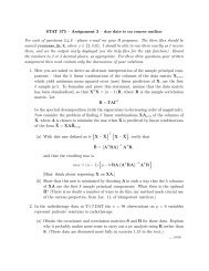
1<br />
Relative efficiency of robust test vs. power; alpha = 0.01<br />
rel. eff.<br />
0.2 0.3 0.4 0.5 0.6 0.7<br />
0.0 0.2 0.4 0.6 0.8 1.0<br />
Beta
70<br />
8. Robustness of test level<br />
• Robustness. How do these tests perform if the<br />
assumptions underly<strong>in</strong>g their derivation are violated?<br />
e.g. <strong>in</strong> the t-test we might assume that<br />
<br />
1 ∼ ³ 2´. How does the test perform<br />
if<br />
(i) the distribution (of ( − ) ) isnon-normal:<br />
perhaps because of contam<strong>in</strong>ation it is<br />
=(1− ) Φ + for some (unknown) , reflect<strong>in</strong>g<br />
a proportion of erroneous sample values;<br />
(ii) the observations are not <strong>in</strong>dependent: perhaps<br />
the <strong>in</strong>dex is ‘time’, and previous observations affect<br />
the current one, as might happen if repeated<br />
measurements are made on the same <strong>in</strong>dividual.
71<br />
• We will consider only ‘level-robustness’. Suppose<br />
we base the construction of the critical region on<br />
the assumption<br />
√ ( − ( 0 )) <br />
→ (0 1)<br />
( 0 )<br />
but <strong>in</strong> fact, when is the true distribution of the<br />
data,<br />
√ ( − ( 0 ))<br />
( 0 )<br />
<br />
→ (0 1)<br />
(Here ( 0 )and ( 0 ) may depend on nuisance<br />
parameters. If we base the test on the assumption<br />
that the data follow a distribution 0 then we<br />
could <strong>in</strong>stead write ( 0 )= 0 ( 0 ).) We reject<br />
if<br />
√ ( − ( 0 ))<br />
<br />
ˆ <br />
where ˆ is a consistent (under ) estimatorof<br />
( 0 )(perhaps ( 0 ) itself, if there are no nuisance<br />
parameters). Take 12, so that <br />
0. Let ( ) be the level of the test, with limit<br />
( ); then
72<br />
( ) = <br />
Ã√ ( − ( 0 ))<br />
ˆ <br />
<br />
!<br />
Thus<br />
Ã√ ( − (<br />
= 0 ))<br />
<br />
( 0 )<br />
Ã<br />
!<br />
(<br />
→ 1 − Φ 0 )<br />
<br />
( 0 )<br />
= 1− Φ ( )+<br />
( ) = +<br />
"<br />
⎧<br />
"<br />
Φ ( ) − Φ<br />
Φ ( ) − Φ<br />
Ã<br />
( 0 )<br />
ˆ <br />
<br />
( 0 )<br />
Ã<br />
(<br />
0 )<br />
<br />
( 0 )<br />
!<br />
<br />
( 0 )<br />
( 0 )<br />
!#<br />
if<br />
⎪⎨<br />
( 0 ) 1<br />
(<br />
is = if 0 )<br />
( 0 ) =1<br />
⎪⎩<br />
(<br />
if 0 )<br />
( 0 ) 1<br />
If ( )is≤ for all <strong>in</strong> a class F of distributions<br />
of the data, we say the test is ‘conservative’ <strong>in</strong> level.<br />
Similarly ‘≥ for all ’is‘liberal’ and‘= for all<br />
’is‘robust’.<br />
!#
73<br />
• Example 1. Suppose we (mistakenly) believe that<br />
asample 1 arises from a ( 2 )population.<br />
We test : = 0 vs. : 0 by<br />
us<strong>in</strong>g the fact that if [] =0 2 then (you<br />
should show)<br />
√ ³<br />
<br />
2 − 0<br />
2 ´ ,r<br />
h ( − ) 2i → (0 1)<br />
This does not require normality of the sample. If<br />
the data are normal, then under ,<br />
h ( − ) 2i =2 4 0 = 2 ( 0 ) <br />
so we can take ˆ = √ 20 2 . Suppose that <strong>in</strong> fact<br />
the sample arises from another distribution with<br />
[] =0 2 but h ( − ) 2i = 2 ( 0).<br />
Then<br />
( 0 )<br />
( 0 ) = √ 2<br />
2<br />
0<br />
( 0 ) <br />
which may take on any positive value. Thus any<br />
( ) ∈ (0 12) is atta<strong>in</strong>able and the test is very<br />
non-robust <strong>in</strong> the class F of distributions with f<strong>in</strong>ite<br />
fourth moment (i.e., non-robust aga<strong>in</strong>st nonnormality).
74<br />
• Example 2. In the same situation as the previous<br />
example, test = 0 . If the are non-normal<br />
but are <strong>in</strong>stead ∼ for <strong>in</strong> the class F of<br />
d.f.s with mean 0 and f<strong>in</strong>ite variance then the<br />
t-statistic (ˆ = ) still tends <strong>in</strong> law to Φ. Thus<br />
( )= and the t-test is robust <strong>in</strong> its level, <strong>in</strong><br />
F. Simulation studies <strong>in</strong>dicate that the approach<br />
of ( )to is quite fast if is symmetric, but<br />
can be quite slow if is skewed. Note that this<br />
example does not contradict the theory above,<br />
s<strong>in</strong>ce here ˆ is consistent not only for ( 0 )=<br />
Φ but for ( 0 ) = , when is the true<br />
distribution.<br />
• Example 3. The result of the previous example<br />
(t-test) is that ( ) → for each fixed ∈<br />
F. A stronger (and more appeal<strong>in</strong>g) form of robustness<br />
requires uniformity (<strong>in</strong> )ofthisconvergence.<br />
This fails drastically; if F is the class of<br />
all distributions with mean 0 ,wehavethatfor<br />
each ,<br />
<strong>in</strong>f ( )=0and sup ( )=1
75<br />
To see this take 0 = 0 for simplicity. Let be the<br />
( 1 1) d.f. and the ( 2 1) d.f. Let =(1−<br />
)+ for ∈ [0 1]; require 1 and 2 to satisfy<br />
(1 − ) 1 + 2 =0 (8.1)<br />
Then ∈ F. Represent the rejection region as ‘X ∈<br />
’, then the level is<br />
( ) = (X ∈ )<br />
=<br />
≥<br />
Z<br />
Y<br />
<br />
=1<br />
(1 − ) Z <br />
{(1 − )( )+( )} 1 ··· <br />
Y<br />
=1<br />
( ) 1 ··· <br />
= (1− ) (X ∈ )<br />
= (1− ) ³√<br />
¯ ≥ ´<br />
<br />
For any this may be made arbitrarily near 1 by choos<strong>in</strong>g<br />
sufficiently small, 1 sufficiently large (how?),<br />
and 2 = −(1 − ) 1 to satisfy (8.1).<br />
That <strong>in</strong>f ( ) = 0 may be shown similarly, by replac<strong>in</strong>g<br />
( )by1− ( )and by its complement,<br />
and then proceed<strong>in</strong>g as above to obta<strong>in</strong><br />
1 − ( ) ≥ (1 − ) ³ √<br />
¯ ´<br />
<br />
(Thanks to J. Sheahan for this second part.)
76<br />
• Robustness aga<strong>in</strong>st dependence. Suppose that<br />
1 are jo<strong>in</strong>tly normally distributed, with<br />
mean , variance 2 . We base a test of = 0<br />
vs. 0 on = √ ³ ¯ − 0´<br />
. We take a<br />
very weak model of dependence, and assume that<br />
the correlations (= ()<br />
<br />
)satisfy(when is<br />
true)<br />
(1)<br />
1<br />
<br />
X<br />
6=<br />
→ (f<strong>in</strong>ite),<br />
1 X<br />
(2)<br />
2 <br />
6=<br />
We calculate, us<strong>in</strong>g (1), that<br />
h √ <br />
³<br />
¯ − 0´i<br />
∙( − 0 ) 2 ³ − 0´2¸<br />
= 2 ⎛<br />
⎝1+ 1 <br />
X<br />
6=<br />
<br />
⎞<br />
⎠<br />
→ 2 (1 + ),<br />
imply<strong>in</strong>g that under , ¯ → 0 <strong>in</strong> and<br />
hence (Corollary 1 of Lecture 1) <strong>in</strong> .<br />
∙<br />
1<br />
<br />
Inthesameway,(2)yieldsthat<br />
1, so<br />
2 = 1 X<br />
( − 0 ) 2 −<br />
<br />
− 1<br />
− 1<br />
P ³ − 0<br />
<br />
´2¸ <br />
→<br />
→ 0<br />
³<br />
¯ − 0´2 <br />
→ 2
77<br />
The numerator of is normally distributed s<strong>in</strong>ce<br />
the are normal, hence it → (0 2 (1 + )).<br />
<br />
It follows that → (0 (1 + )), and that the<br />
level of the t-test (carried out assum<strong>in</strong>g <strong>in</strong>dependence)<br />
is<br />
( ) = <br />
→<br />
Ã<br />
1 − Φ<br />
<br />
√ 1+<br />
<br />
Ã<br />
!<br />
<br />
√ 1+<br />
!<br />
<br />
√ (8.2)<br />
1+<br />
• Example: AR(1). Suppose that : =0is<br />
true but that, <strong>in</strong>stead of be<strong>in</strong>g <strong>in</strong>dependent, the<br />
follow a stationary AR(1) model:<br />
+1 = + +1 (|| 1)<br />
(8.3)<br />
where { } is ‘white noise’, i.e. i.i.d. (0).<br />
2<br />
We carry out a t-test and reject if = √ ¯ <br />
. If (1) and (2) hold then so does (8.2). To verify<br />
(1) note that 2 = 2 ³ 1 − 2´<br />
(derived <strong>in</strong>
78<br />
text)and,asabove,1+ =lim h √ ¯ i 2 .<br />
Sum (8.3) over =1 − 1toget<br />
√ ¯ = + √ ¯<br />
<br />
1 − <br />
where =( 1 − − 1 ) √ .S<strong>in</strong>ce<br />
¯<br />
¯ ³ √ r<br />
¯´¯¯¯ ≤ [ ] h √ i<br />
¯<br />
and [ ] → 0, we have<br />
lim h √ ¯ i = lim [√ ¯]<br />
(1 − ) 2 = 2 <br />
(1 − ) 2<br />
This results <strong>in</strong> 1 + = 1+<br />
1−<br />
, which varies over<br />
all of (0 ∞) (so the asymptotic level varies over<br />
(05)) as varies over (−1 1). (Condition (2)<br />
— equivalently, that <br />
∙<br />
1<br />
<br />
P ³ − 0<br />
<br />
´2¸<br />
→ 0—<br />
can be established <strong>in</strong> the same way; this is left to<br />
you.)<br />
The t-test is very non-robust aga<strong>in</strong>st even very<br />
weak dependencies of this form.
79<br />
9. Confidence <strong>in</strong>tervals<br />
• X =( 1 ) the data, from a distribution<br />
parameterized by . An <strong>in</strong>terval [(X) ¯(X)] is<br />
an asymptotic 1 − confidence <strong>in</strong>terval (CI) if<br />
<br />
³<br />
≤ ≤ ¯´ → 1 − , for each <br />
It is a strong CI if<br />
<strong>in</strong>f ³<br />
≤ ≤ ¯´<br />
→ 1 − <br />
<br />
entail<strong>in</strong>g a form of uniformity <strong>in</strong> the convergence.<br />
(Strictly speak<strong>in</strong>g, uniformity has convergence of<br />
both <strong>in</strong>f and sup.)<br />
— We can replace by <strong>in</strong> the above, where<br />
is a nuisance parameter; the <strong>in</strong>f <strong>in</strong> the def<strong>in</strong>ition<br />
of strong CI is then taken over ( ).<br />
— Relationship to tests: We can reject : =<br />
0 <strong>in</strong> favour of : 6= 0 iff 0 ∈ [ ¯], this<br />
def<strong>in</strong>es a level test, asymptotically.
80<br />
• An example of a strong CI: 1 <br />
<br />
∼ ( 2 ).<br />
The CI derived from the 2-sided t-test is ¯ ±<br />
2 √ ,with<br />
¯ − <br />
( ∈ ) = <br />
ﯯ¯¯ √ ¯ ≤ 2<br />
= ³ | −1 | ≤ 2´<br />
→ 1 − ;<br />
s<strong>in</strong>ce the probability does not depend on the parameters<br />
the convergence is uniform.<br />
— The above is typical when the CI is based on<br />
a ‘pivot’ — a function of the data and of the<br />
parameter whose distribution does not depend<br />
on the parameters.<br />
¯<br />
!
81<br />
• Example. 1 ∼ () ( 0); test<br />
= 0 . The large-sample test has acceptance<br />
¯<br />
region ¯√ ³ ¯ − 0´<br />
√ 0¯¯¯ ≤ 2 ,equivalently<br />
³ ¯ − 0´2<br />
≤ <br />
2<br />
2<br />
0 , result<strong>in</strong>g <strong>in</strong> the CI with<br />
endpo<strong>in</strong>ts<br />
¯ + 2 2<br />
2 ± 2<br />
√ <br />
v uut<br />
¯ + 2 2<br />
4 (9.1)<br />
Replac<strong>in</strong>g √ 0 by √ ¯ <strong>in</strong> the test statistic leads<br />
<strong>in</strong>stead to the CI<br />
¯ ± 2<br />
s<br />
¯<br />
<br />
which agrees with the previous one up to terms<br />
which are ( −1 ) (i.e. if such terms are dropped).<br />
This <strong>in</strong>terval is not strong. Toseethis,notethat<br />
¯ − 2<br />
r<br />
¯<br />
<br />
≤ ≤ ¯ + 2<br />
r<br />
¯<br />
<br />
implies that<br />
¯ 0, hence<br />
⎛ s s ⎞<br />
⎝<br />
¯<br />
¯<br />
<br />
¯ − 2<br />
≤ ≤ ¯ + ⎠ 2<br />
<br />
≤ 1 − <br />
³<br />
¯ =0´ =1− − → 0as → 0
82<br />
hence<br />
<strong>in</strong>f ³<br />
( ∈ ) ≤ <strong>in</strong>f 1 − <br />
−´<br />
=0<br />
0<br />
(If is known to be bounded away from 0 then<br />
this example fails and the required uniformity holds<br />
—derivation<strong>in</strong>text,basedonBerry-Esséen.)<br />
— The same argument shows that (9.1), which<br />
=<br />
∙0 ¸<br />
2 2<br />
if ¯ = 0, is also not strong if<br />
³<br />
<strong>in</strong>f <br />
2<br />
2<br />
1 − <br />
−´<br />
=1− −2 2<br />
1−<br />
( ' 215 will suffice).<br />
— In (either form of) this Poisson example, note<br />
that (with AN test statistic ())<br />
<strong>in</strong>f lim<br />
( ∈ )<br />
= <strong>in</strong>f lim<br />
³<br />
−2 ≤ () ≤ 2´<br />
³<br />
= <strong>in</strong>f −2 ≤ ≤ 2´<br />
Φ<br />
= 1− <br />
but this is not enough for a strong CI; we need<br />
lim <strong>in</strong>f ( ∈ ) =1− —theoperations<br />
are <strong>in</strong>terchanged.
83<br />
• A strong CI on a population median. Suppose<br />
1 are a sample from , with unique median<br />
= −1 (5). (Here is viewed as a nuisance<br />
parameter.) Recall that the sample median<br />
ˆ is ³ 1 ³ 4 2 ()´´, but a CI based on<br />
this requires a knowledge of . Consider <strong>in</strong>stead<br />
the follow<strong>in</strong>g procedure based on the b<strong>in</strong>omial distribution.<br />
We test = 0 (2-sided) us<strong>in</strong>g the sign<br />
test, with test statistic<br />
( 0 ) = # of observations which are 0 <br />
We accept if ≤ ( 0 ) ≤ − .Notethat<br />
= − ⇔ obs’ns are ≤ 0 ⇔ 0 ∈ [ () (+1) )<br />
so that<br />
⇔<br />
≤ ( 0 ) ≤ − <br />
0 ∈∪ − <br />
= <br />
[ () (+1) )=[ ( ) (− +1) )<br />
Under , ∼ ( 12); thus 2 √ ³ <br />
Φ and we determ<strong>in</strong>e by requir<strong>in</strong>g that<br />
⎛<br />
⎝ 2√ ³ − 1 ´ √ ³<br />
2 ≤ 2 <br />
≤ 2 √ ³ − <br />
<br />
− 1 ´<br />
2<br />
→ 1 − <br />
<br />
− 1 2<br />
<br />
− 1 2<br />
´<br />
⎞<br />
⎠<br />
´ →
84<br />
√<br />
This holds if = 2 − 2<br />
2<br />
(+( √ )), then<br />
the →− 2 and the → 2 . We<br />
∙<br />
<br />
2<br />
−<br />
√<br />
2<br />
2<br />
can take =<br />
or use any other<br />
round<strong>in</strong>g mechanism. Now<br />
³<br />
( ) ≤ 0 (− +1)´<br />
0 <br />
= ( ≤ ( 12) ≤ − )<br />
→ 1 − <br />
uniformly <strong>in</strong> 0 and , s<strong>in</strong>ce it depends only on<br />
. ThusastrongCIis[ ( ) (− +1) ).<br />
¸
85<br />
• A more <strong>in</strong>volved example of a strong CI. Suppose<br />
we have two <strong>in</strong>dependent samples: 1 ∼<br />
( 2 )and 1 ∼ ( 2 ); def<strong>in</strong>e =<br />
− . Put =( 2 2 ) (nuisance parameter)<br />
and let ˆ 2 and ˆ 2 bethesamplevariances. An<br />
asymptotic level 2-sided test ( →∞; put<br />
= + ) has acceptance region<br />
where<br />
|| √ =<br />
= () =<br />
= ¯ − ¯ − <br />
r<br />
2<br />
+ 2<br />
<br />
¯<br />
¯ − ¯ − <br />
r<br />
ˆ 2<br />
+ ˆ 2<br />
<br />
¯<br />
≤ 2 <br />
È<br />
2<br />
+ ˆ 2 !,Ã<br />
<br />
2<br />
+ 2 !<br />
<br />
are <strong>in</strong>dependent,<br />
and<br />
and is distributed as (0 1) (free of any parameters!).
86<br />
Thus, for any 0,<br />
( ∈ )<br />
³ √<br />
= || ≤ 2 ´<br />
( ³ √<br />
|| ≤ 2 || − 1| ´<br />
·<br />
=<br />
(| − 1| )<br />
( ³ √<br />
|| ≤ 2 || − 1| ≥ ´<br />
·<br />
+<br />
(| − 1| ≥ )<br />
so that<br />
=<br />
≤<br />
≤<br />
¯<br />
¯ ( ∈ ) − (1 − )<br />
¯<br />
¯ ≤<br />
³ √<br />
|| ≤ 2 || − 1| ´<br />
·<br />
(| − 1| ) − (1 − ) ¯<br />
+ (| − 1| ≥ )<br />
<br />
¯<br />
= ¯ · − (1 − ) ¯ + ³ 1 − ´<br />
³ ³<br />
¯<br />
¯ − (1 − ) − 1 − ´¯¯¯ + 1 − ´<br />
¯<br />
¯<br />
¯ − (1 − ) ¯ + ³ 1+ ´³<br />
1 − ´<br />
¯<br />
¯<br />
¯ − (1 − ) ¯ +2 ³ 1 − ´<br />
(9.2)<br />
¯<br />
)<br />
)
87<br />
We exhibit 1 () 2 () → 1− and ()<br />
→0<br />
such that<br />
→ 1<br />
→∞<br />
³ √<br />
1): 1 () ≤ || ≤ 2 || − 1| ´<br />
≤ 2 ()<br />
2): (| − 1| ) ≥ () <br />
Then (9.2) is, uniformly <strong>in</strong> , ≤<br />
() = max{| 1 () − (1 − )| | 2 () − (1 − )|}<br />
+2 (1 − ()) <br />
Now () → max {| 1 () − (1 − )| | 2 () − (1 − )|}<br />
as →∞, and this may be made arbitrarily small.<br />
For 1) note that <br />
³<br />
|| ≤ 2<br />
√<br />
|| − 1| ´<br />
is maximized by choos<strong>in</strong>g aslargeaspossible(=<br />
1+), yield<strong>in</strong>g 2 () =2Φ ³ 2<br />
√ 1+´<br />
− 1, and<br />
similarly 1 () =2Φ ³ √<br />
2 1 − ´<br />
− 1. Here we use<br />
the <strong>in</strong>dependence of and . Both these bounds<br />
→ 1 − as → 0.
88<br />
For 2), write<br />
=<br />
È<br />
2<br />
+ ˆ 2 !,Ã<br />
<br />
2<br />
+ 2 !<br />
<br />
= ˆ2<br />
2<br />
+(1− )ˆ<br />
2 2<br />
= +(1− ) <br />
Áµ<br />
2<br />
+ 2<br />
<br />
<br />
,where and are distrib-<br />
for = 2<br />
<br />
uted <strong>in</strong>dependently of any parameters (<strong>in</strong> particular,<br />
<strong>in</strong>dependently of ) and→ 1 Then (| − 1| )<br />
is<br />
= (| ( − 1) + (1 − )( − 1) | )<br />
≥ (| − 1| +(1− )| − 1| )<br />
≥ (| − 1| and | − 1| )<br />
<br />
= () → 1, free of and hence uniformly.
10. Po<strong>in</strong>t estimation; <strong>Asymptotic</strong> relative efficiency<br />
89<br />
• Po<strong>in</strong>t estimation. Suppose that a statistic is<br />
computed as an estimate of a function (), and<br />
that it is AN:<br />
à !<br />
√ − ()<br />
<br />
<br />
<br />
→ (0 1)<br />
We take as a measure of the accuracy of ,<br />
s<strong>in</strong>ce it is proportional to the width of an asymptotic<br />
CI.<br />
• <strong>Asymptotic</strong> variance vs. limit<strong>in</strong>g variance:<br />
asymptotic variance is<br />
The<br />
2 0 = lim 2 (or plim ˆ 2 <strong>in</strong>thecaseofstudentiz<strong>in</strong>g),<br />
if the limit exists. Then<br />
<br />
<br />
= √ ( − ()) → (0 2 0 )<br />
It can be shown that the limit<strong>in</strong>g variance (when<br />
it exists, otherwise use lim <strong>in</strong>f) exceeds the asymptotic<br />
variance:<br />
lim ( ) ≥ 2 0
90<br />
—Example: Let ∼ ( ) <strong>in</strong>dependently<br />
of ∼ (1 )with → 1. Def<strong>in</strong>e<br />
= − <br />
√ + (1 − ) <br />
<br />
Then <br />
→ (0<br />
2<br />
0 = (1 − )) (why?) but<br />
( ) ≥ ( [ | ])<br />
= [ (1 − )]<br />
= () 2 (1 − )<br />
and this →∞if → 1slowly,say =<br />
1 − 1.<br />
• Exampleslikethisaretroublesomes<strong>in</strong>cewewould<br />
like to use the, more convenient, asymptotic variance<br />
as a measure of accuracy. Fortunately it is<br />
typically the case that the two quantities agree.<br />
Conditions under which they agree are given <strong>in</strong><br />
the follow<strong>in</strong>g result, <strong>in</strong> which we assume that<br />
1 are i.i.d., with mean and variance<br />
2 ,andthat = ( ¯).
91<br />
Recall that if 0 () 6= 0 (assumed), then<br />
√ ³ µ<br />
( ¯) − ()´<br />
→ 00 2 = ³ 0 ()´2 <br />
Thus we aim to establish that<br />
lim ³ √ ( ¯)´<br />
= ³ 0 ()´2 <br />
(10.1)<br />
We assume that the have a f<strong>in</strong>ite fourth moment;<br />
this implies that<br />
(Proof of (i): <br />
= −3 <br />
= −3 <br />
∙ ³<br />
(i) ¯ − ´3¸<br />
∙ ³<br />
(ii) ¯ − ´4¸<br />
∙ ³<br />
¯ − ´3¸<br />
⎡<br />
⎣ X<br />
<br />
⎡<br />
⎣ X <br />
= ( −2 )<br />
= ( −2 )<br />
( − ) ³ − ´ ( − )<br />
( − ) 3 ⎤<br />
⎦ = ( −2 )<br />
s<strong>in</strong>ce the only nonzero terms are those <strong>in</strong> which all<br />
three <strong>in</strong>dices agree. Assertion (ii) is proven similarly.)<br />
⎤<br />
⎦
Theorem: Assume the conditions above, and that <br />
is four times differentiable. We have:<br />
(i) if (4) is bounded, then<br />
h ( ¯) i = ()+ 2<br />
2 00 ()+( −2 );<br />
(ii) if both (4) and ( 2 ) (4) arebounded,then<br />
92<br />
h ( ¯) i = 2 ³<br />
0 ()´2 + ( −2 )<br />
<br />
(so that <strong>in</strong> particular (10.1) holds).<br />
Proof: We prove (i); for (ii) one writes h ( ¯) i<br />
as h 2 ( ¯) i − ³ h ( ¯) i´2 and applies (i) to each<br />
component. By Taylor’s Theorem,<br />
³<br />
¯ − ´2<br />
( ¯) = ()+ 0 () ³ ¯ − ´ + 00 ()<br />
2<br />
³ ³<br />
¯ − ´3<br />
¯ − ´4<br />
+ 000 () + (4) ()<br />
3!<br />
for some between ¯ and . Then<br />
4!<br />
<br />
h ( ¯) i = ()+ 00 () 2<br />
2 +
93<br />
where (with be<strong>in</strong>g a bound on<br />
| | =<br />
≤<br />
∙ ³<br />
¯ − ´3¸<br />
000 ()<br />
3!<br />
+ <br />
¯<br />
¯<br />
¯ 000 ()<br />
¯<br />
¯<br />
= ( −2 )<br />
<br />
∙ ³<br />
¯ − ´3¸<br />
3!<br />
¯<br />
¯<br />
¯<br />
¯ (4) () ¯),<br />
⎡<br />
⎢<br />
⎣ (4) ()<br />
+ <br />
¯<br />
³<br />
¯ − ´4<br />
4!<br />
∙ ³<br />
¯ − ´4¸<br />
4!<br />
⎤<br />
⎥<br />
⎦<br />
¯<br />
¯<br />
• Why the fourth derivative, not merely the third?<br />
• Example: The theorem applies to the case ∼<br />
( 1) and () = ( ≤ ) =Φ( − ). The<br />
limit<strong>in</strong>g and asymptotic variances of √ ( ¯) =<br />
√ Φ( − ¯) areboth £ 0 () ¤ 2 = 2 ( − ).
94<br />
• When is less well-behaved, ad hoc methods are<br />
<br />
required. Let 1 ∼ ( 1) and estimate<br />
() = by ( ¯). The derivatives of <br />
are unbounded so the theorem above does not<br />
apply. But<br />
√ ³ h ( ¯) − ()´ → (0 0 () i 2<br />
= 2 )<br />
and<br />
√ ( ¯) = √ ¯ = √ ¯−<br />
has variance 2 var h √ ¯− i , so we have equality<br />
of the limit<strong>in</strong>g and asymptotic variances if<br />
var h ¯− i → 1. With √ ³ ¯ − ´<br />
= ∼<br />
(0 1) and () = h i = 22 we have that<br />
var<br />
∙ ¯−¸ = · var h √ i<br />
= n h 2√ i − 2 h √ io<br />
= n (2 √ ) − 2 (1 √ ) o<br />
= n 2 − 1o (exactly!)<br />
= <br />
½∙1+ 2 + ³ −2´¸<br />
−<br />
∙1+ 1 + ³ −2´¸¾<br />
<br />
= 1+ ³ −1´<br />
as required.
• <strong>Asymptotic</strong> Relative Efficiency.<br />
two estimators 1 2 of () have<br />
95<br />
Suppose that<br />
[ ] = ()+ <br />
+ (−2 )<br />
[ ] = <br />
2 + (−2 )<br />
(In the Theorem we had = ( ¯), = 2 00 ()2<br />
and 2 = £ 0 () ¤ 2 .) Then [ ]=( −1 )<br />
and<br />
[ ]= 2 + = <br />
2 + (−2 )<br />
In order that the two estimators have the same<br />
asymptotic MSE, i.e. 1<br />
2<br />
<br />
∼ 2<br />
2<br />
1 <br />
,itisrequiredthat<br />
2<br />
1<br />
2<br />
→ 2 1<br />
2 2<br />
<br />
= 21 <br />
the ARE of 2 with respect to 1 . (We can use<br />
the asymptotic variances rather than the limit<strong>in</strong>g<br />
variances; of course these typically agree.)<br />
— Does this agree with the previous def<strong>in</strong>ition <strong>in</strong><br />
terms of efficacies?
96<br />
• Example: Estimate ( ≤ ) = () froma<br />
sample 1 . If is the ( 1) d.f. then<br />
() =Φ( − ) =(). We take 1 = ( ¯)<br />
with 1 2 = £ 0 () ¤ 2 = 2 ( − ).<br />
One might <strong>in</strong>stead use the ‘plug-<strong>in</strong>’ estimate:<br />
2 = ˆ () = # { ≤ } ( ())<br />
∼ <br />
<br />
<br />
2 2 = ()[1− ()] = Φ( − )[1− Φ( − )] <br />
Then<br />
2 ( − )<br />
21 =<br />
Φ( − )[1− Φ( − )] <br />
Some calculus shows that this is maximized at<br />
− =0,with<br />
2 (0)<br />
21 ≤<br />
Φ(0) [1 − Φ(0)] =42 (0) = 2 ≈ 64<br />
Thus the MLE 1 requires fewer than 23 asmany<br />
observations for an asymptotic CI of the same<br />
width (many fewer if | − | is even moderately<br />
large).<br />
Does this mean that 1 is necessarily preferred for<br />
estimat<strong>in</strong>g ( ≤ )? Why or why not?
97<br />
0.0 0.1 0.2 0.3 0.4 0.5 0.6<br />
-3 -2 -1 0 1 2 3<br />
x<br />
2 ()<br />
Φ()[1−Φ()]<br />
vs.
98<br />
11. Compar<strong>in</strong>g estimators<br />
• Example: Estimat<strong>in</strong>g a centre of symmetry.<br />
<br />
1 ∼ ( − ) for a symmetric d.f.<br />
with f<strong>in</strong>ite variance. Consider the compet<strong>in</strong>g<br />
estimators (i) Mean ¯ with 2¯ = 2 <br />
and (ii)<br />
Median ˜ with 2˜ = 1 The ARE of the<br />
4 2 (0) .<br />
median w.r.t. the mean is ˜ ¯ = 42 2 (0).<br />
Recall that this is also the ARE of the sign test<br />
to the t-test. It may be <strong>in</strong>f<strong>in</strong>itely large; at = Φ<br />
it is 2 ≈ 64<br />
• In the framework of the preced<strong>in</strong>g example a compromise<br />
is the trimmed mean, i.e. the average of<br />
the middle − 2 observations. Put = <br />
5, then the estimate is<br />
¯ = 1 ³<br />
(+1) + + <br />
− 2<br />
(−)´<br />
<br />
Suppose that has a density , cont<strong>in</strong>uous and<br />
positive where 0 () 1. It can be shown
99<br />
that then √ ³ ¯ − ´ → (0<br />
2 )where,with<br />
= −1 (1 − ),<br />
2 = <br />
h<br />
m<strong>in</strong> (|| ) 2i (1 − 2) 2<br />
=<br />
" Z<br />
2 <br />
(1 − 2) 2 2 () + <br />
2 0<br />
This reduces to 2 as → 0( →∞). Here<br />
we use that<br />
2 = h<br />
||<br />
2 i<br />
h<br />
≥ m<strong>in</strong> (|| ) 2i<br />
= (1− 2) 2 2 (11.1)<br />
= 2<br />
" Z <br />
0<br />
2 () + 2 <br />
so that 2 → 0as → 0. As → 12, 2 →<br />
1 h 4 2 (0) i , by two applications of L’Hospital’s<br />
rule.<br />
#<br />
<br />
#
100<br />
• We have ¯ ¯ = 2 2 .Thisis 1formoderate<br />
and distributions with heavier than normal<br />
tails, e.g. on a small number of d.f. By (11.1),<br />
¯ ¯<br />
≥ (1 − 2)2<br />
for any symmetric d.f. with f<strong>in</strong>ite variance.<br />
• A compet<strong>in</strong>g estimate of a centre of symmetry is<br />
the Hodges-Lehmann estimate ˆ = <br />
µ<br />
+ <br />
2<br />
where the median is over all pairs ≤ or (asymptotically<br />
equivalently) .Itcanbeshown<br />
that<br />
√ <br />
³ˆ − ´ → <br />
Ã<br />
0 1<br />
(<br />
12<br />
∙Z<br />
¸2)!<br />
2 () <br />
<br />
,<br />
with<br />
¯ =122 <br />
∙Z<br />
2 ()¸2
101<br />
— This is also the ARE of the Wilcoxon test to<br />
the t-test.<br />
Connection: Suppose we test : = 0 (2-<br />
sided) with ( 0 ) as test statistic, reject<strong>in</strong>g for<br />
large . As an estimate we can take ˆ =the<br />
0 which m<strong>in</strong>imizes ( 0 ), i.e. the value of the<br />
parameter least likely to be rejected. (For the<br />
-test ( 0 )= √ ¯ ¯ − 0¯¯¯ is m<strong>in</strong>imized<br />
at 0 = ¯; forthesigntest<br />
( 0 ) = |{# ofobs’ns 0 } − 12|<br />
= 1<br />
{# ofobs’ns 0 }<br />
2 ¯ − {# ofobs’ns 0 } ¯<br />
is m<strong>in</strong>imized by what?) The HL estimate<br />
arises <strong>in</strong> the same way from the one-sample<br />
Wilcoxon test (which is based on the sum of<br />
the ranks of those | − 0 | for which −<br />
0 0); this is a consequence of Problem 4<br />
on asst. 2.
102<br />
• For any symmetric, square <strong>in</strong>tegrable density <br />
with variance 2 , ¯ ≥ 864<br />
Proof: Put () =12<br />
2 h R<br />
2 () i 2<br />
and () =<br />
( ), with unit variance ( 2 =1). Then<br />
() =12<br />
∙Z<br />
2 ()¸2<br />
= ()<br />
so we can take =1. Wearethento<br />
m<strong>in</strong>imize<br />
Z<br />
Z<br />
2 () =1<br />
2 () subject to<br />
Z<br />
() =1<br />
with symmetric and non-negative.<br />
It is sufficient that = (; ) m<strong>in</strong>imize<br />
Z<br />
2 () +2<br />
Z<br />
2 () − 2<br />
Z<br />
()<br />
unconditionally, for constants (‘Lagrange multipliers’)<br />
, and satisfy the side conditions. (Why?<br />
It is very <strong>in</strong>structive to write out the details of the<br />
argument.)
103<br />
We m<strong>in</strong>imize<br />
Z h<br />
2 ()+2 2 () − 2() i <br />
by m<strong>in</strong>imiz<strong>in</strong>g the <strong>in</strong>tegrand po<strong>in</strong>twise: 2 − (2 −<br />
2 2 ) is m<strong>in</strong>imized over ≥ 0by =( − 2 ) + ;<br />
thus<br />
() =( − 2 ) + <br />
which is symmetric and non-negative. Necessarily <br />
0 for <strong>in</strong>tegrability; then also 0else ≡ 0. Thus<br />
we can write as<br />
à !<br />
() = 1 − 2<br />
2 || ≤ <br />
Thesidecondition R () =1gives =3(4) and<br />
then R 2 () =1gives = √ 5; thus<br />
Ã<br />
() = 3<br />
4 √ 5<br />
1 − 2 5<br />
|| ≤ √ 5<br />
and we calculate that<br />
" Z<br />
√ # 2 5<br />
() =12<br />
− √ 2 () = 108<br />
5 125 = 864<br />
If has this density then 2 5 ∼ (12 2).<br />
!
104<br />
12. Biased estimation; Pitman closeness<br />
• Biased estimation. In general, to compare estimators<br />
1 2 of () with variances 2 () and<br />
biases () welookattheARE<br />
2 1<br />
= lim ( 1)<br />
( 2 ) = lim ( 1)+ 2 ( 1 )<br />
( 2 )+ 2 ( 2 ) <br />
In the examples studied previously 2 was of<br />
order ( −2 ) and the ARE reduced to a comparison<br />
of the limit<strong>in</strong>g, or asymptotic, variances. We<br />
look below at an example <strong>in</strong> which and 2<br />
are of the same order, and <strong>in</strong> which 2 plays a<br />
significant role, asymptotically. First we look at<br />
another measure of performance of an estimator.<br />
• A related measure of accuracy is ‘Pitman closeness’<br />
(| − | ≤ ) for specified ; onewants<br />
this probability to be large. For an asymptotic<br />
treatment we would typically have to normalize,<br />
and consider someth<strong>in</strong>g like lim ( √ | − | ≤ ).
105<br />
In a broad class of cases, comparisons based on Pitman<br />
closeness of two estimators reduce to compar<strong>in</strong>g<br />
the (exact or asymptotic) biases. Suppose that <br />
is the d.f. of ( − []) , andthat is symmetric<br />
about 0 with a unimodal density (i.e. is a decreas<strong>in</strong>g<br />
function of ||). Then with (bias) = []− <br />
we have that the Pitman closeness is<br />
(| − | ≤ ) =<br />
µ ∙ µ ¸<br />
− <br />
+ <br />
− 1 − <br />
<br />
<br />
= ()<br />
say. This is an even function of whose derivative is<br />
µ µ ¸<br />
() =<br />
∙<br />
−1 + − <br />
− <br />
<br />
<br />
This (odd) function of is 0if0 (s<strong>in</strong>ce then<br />
| + | | − |); thus under these conditions the<br />
Pitman closeness is a decreas<strong>in</strong>g function of || for<br />
any 0.<br />
Thus <strong>in</strong> compar<strong>in</strong>g two estimators, for each of which<br />
( − []) ∼ exactly or asymptotically (same ,<br />
same ) the estimate with smaller (absolute) bias ||<br />
— hence smaller mse — is Pitman closer.
106<br />
This conclusion (smaller mse ⇒ Pitman closer) need<br />
not hold without these assumptions. The conclusion<br />
smaller mse ⇔ smaller variance need not hold either.<br />
Suppose 1 are i.i.d. (0). Consider estimates<br />
= () of . With = ( +1)<br />
we have unbiasedness. We compare (+1) to 1<br />
with ³ respect to both mse and Pitman closeness. From<br />
() ≤ ´<br />
=() we calculate that h i =<br />
<br />
+ () then obta<strong>in</strong> the bias, variance and mse:<br />
µ <br />
( ) =<br />
+1 − 1 <br />
à µ !<br />
( ) = 2 2<br />
+2 − 2 <br />
+1<br />
∙<br />
( ) = 2 <br />
+2 − 2 +1¸<br />
2 <br />
+1<br />
Note mse is m<strong>in</strong>imized by =( +2)( +1). Both<br />
this and =( +1) satisfy ( − 1) → 1; we shall<br />
handle both cases by compar<strong>in</strong>g 1 with ∗,where<br />
( ∗ − 1) → 1. For arbitrary , werewritethemse<br />
as<br />
h<br />
( ( − 1))<br />
2 +1<br />
<br />
( )=<br />
− 2 ( − 1) + 2i 2<br />
<br />
( +1)( +2)
107<br />
The ARE of the estimates considered, based on mse,<br />
is<br />
( ∗ 1 ) = lim ( 1)<br />
( ∗) = lim 2<br />
h +1<br />
− =2<br />
2+2i<br />
Thus any such ∗ has 12 themse, asymptotically,<br />
even though ( ∗) ( 1 )if ∗ 1. (Both bias 2<br />
and variance of 1 are ( −2 ) and so reduc<strong>in</strong>g the<br />
bias effects a significant reduction <strong>in</strong> mse, even asymptotically.)<br />
• To<br />
³<br />
compare<br />
³<br />
w.r.t. Pitman closeness, recall that<br />
− ()´<br />
≤ ´<br />
→ 1 − − =1− − ,<br />
with = . Then the Pitman closeness is<br />
= <br />
µ<br />
| − | ≤ <br />
= <br />
µ<br />
− ≤ () − ≤ <br />
= <br />
⎛<br />
⎝<br />
−+(−1)<br />
<br />
<br />
<br />
≤ ³ − ()´<br />
≤ +(−1)<br />
<br />
⎞<br />
⎠
108<br />
with<br />
1 =<br />
³ ³<br />
− ≤ − ()´<br />
≤ ´<br />
→ 1 − − ³<br />
<br />
³<br />
∗ → lim − + ≤ − ()´<br />
≤ + ´<br />
(<br />
1 − <br />
=<br />
1<br />
−1 − −−1 ≤ 1<br />
= m<strong>in</strong> ³ 1 −1´ − −−1 <br />
0.0 0.05 0.10 0.15 0.20<br />
0.0 0.5 1.0 1.5 2.0<br />
r<br />
Values of lim →∞ { ∗ () − 1 ()} vs. . The<br />
unbiased or m<strong>in</strong>imum mse estimate ∗ is<br />
asymptotically Pitman closer than 1 only for<br />
= log( − 1) ≈ 541. Note that the<br />
comparison depends on the values of and .
109<br />
We have lim →∞ { ∗ () − 1 ()} 0( ∗ is<br />
asymptotically Pitman closer) if<br />
m<strong>in</strong> ³ 1 −1´ − −−1 1 − − <br />
This holds if<br />
(i) 1, or if<br />
(ii) ≤ 1and −1 − −−1 1 − − ,i.e.the<br />
function<br />
() = −1 ³ − −´ + − − 1<br />
has () 0(01). Equivalently, with<br />
= 1, we need<br />
(i) ,or<br />
(ii) 1 ≤ and () = (−1)(−(−1))<br />
<br />
0.<br />
The second condition holds for ∈ ( − 1], and<br />
so the requirement is merely − 1. Equivalently,<br />
= log( − 1) ≈ 541.
110<br />
Part III<br />
MULTIVARIATE<br />
EXTENSIONS
111<br />
13. Random vectors; multivariate normality<br />
• Convergence <strong>in</strong> probability of random vectors.<br />
Let X () be a sequence of × 1 random vectors,<br />
with elements () (r.v.s) =1. We say<br />
X<br />
() <br />
<br />
→ c if ³ ||X () − c|| ≥ ´ → 0 for every<br />
0. Equivalently (you should show) () <br />
<br />
→ <br />
for each . Exactly as <strong>in</strong> the univariate case, if f :<br />
R → R is cont<strong>in</strong>uous at c and X<br />
() <br />
→ c then<br />
f ³ X ()´ <br />
→ f (c). In particular, t 0 X<br />
() <br />
→ t 0 c for<br />
vectors t<br />
• Convergence <strong>in</strong> law. Let ⊆ R .Theboundary<br />
of is the set of all po<strong>in</strong>ts x such that any<br />
open ball around x <strong>in</strong>tersects both and .We<br />
say X () ³<br />
→ X ∼ if X () ∈ ´ → (X ∈<br />
) whenever is a product (−∞ 1 ] ×···×<br />
(−∞ ]and () = 0. Note this agrees<br />
with the previous ( = 1) def<strong>in</strong>ition s<strong>in</strong>ce the<br />
boundary of (−∞] <strong>in</strong> R is the po<strong>in</strong>t , and<br />
({}) =0meansthat is a cont<strong>in</strong>uity po<strong>in</strong>t
112<br />
of . Anequivalent(andmoreuseful)def<strong>in</strong>ition<br />
is that<br />
X () → X ⇔ <br />
h<br />
<br />
³<br />
X ()´i → [ (X)] <br />
whenever is bounded and cont<strong>in</strong>uous.<br />
• If X () → X and f(·) is cont<strong>in</strong>uous then<br />
f ³ X ()´ () <br />
→ f (X); <strong>in</strong> particular <br />
<br />
→ (∀).<br />
Proof: Let be bounded and cont<strong>in</strong>uous, then<br />
h ³ f ³ X ()´´i → [ (f (X))] s<strong>in</strong>ce ◦ f is<br />
bounded and cont<strong>in</strong>uous.<br />
• That ()<br />
<br />
()<br />
<br />
<br />
→ (∀) ⇒ X () → X holds if the<br />
are <strong>in</strong>dependent r.v.s; similar to a current<br />
exercise there is an easy proof us<strong>in</strong>g c.f.s which<br />
leads to the additional conclusion that the components<br />
of X are <strong>in</strong>dependently distributed.
113<br />
• X ()<br />
()<br />
<br />
→ c (constant) ⇒ <br />
()<br />
<br />
→ (∀) ⇒ X<br />
() <br />
→ c.<br />
<br />
<br />
→ <br />
(∀) ⇒<br />
• Characteristic functions: X (t) = £ exp ¡ t 0 X ¢¤ <br />
( real).<br />
— Uniqueness: If X (t) = Y (t) forallt then<br />
X ∼ Y.<br />
— Convergence: X () → X ⇔ X ()(t) → X (t)<br />
for all t.<br />
• Cramér-Wold device:<br />
⇔<br />
⇔<br />
X () → X<br />
h exp ³ t 0 X ()´i → h exp ³ t 0 X´i for all t<br />
h exp ³ t 0 X ()´i → h exp ³ t 0 X´i for all t<br />
⇔ t 0 X () → t 0 X for all t;<br />
i.e. we have convergence <strong>in</strong> law of X () to X iff<br />
all l<strong>in</strong>ear comb<strong>in</strong>ations of X () converge <strong>in</strong> law to<br />
those of X.
114<br />
• Slutsky’s Theorem: If X () → X and the elements<br />
of the × matrices A () and ×1 vectors<br />
b () converge <strong>in</strong> probability to the correspond<strong>in</strong>g<br />
(constant) elements of A and b, then<br />
Proof:<br />
A () X () + b () → AX + b<br />
We will prove<br />
X () → X<br />
⎫<br />
⎪⎬<br />
Y () <br />
→ c (constant) ⎪⎭ ⇒ ³ X () Y ()´ → (X c) <br />
(13.1)<br />
Apply this with Y () = ³ A () b ()´<br />
and f the<br />
cont<strong>in</strong>uous function f ³ X () Y ()´ = A () X () +<br />
b () ,whichthen→ f (X c) =AX + b.<br />
To prove (13.1) first use the Cramér-Wold device<br />
to reduce it to the statement ‘ → ,<br />
<br />
<br />
<br />
→ ⇒ + → + ’; this special case<br />
oftheunivariateSlutsky’sTheoremwasproven<br />
<strong>in</strong> Assignment 1.<br />
• A consequence of Slutsky’s Theorem, established<br />
exactly as <strong>in</strong> the univariate case, is that<br />
X<br />
() <br />
→ X ⇒ X () → X
115<br />
• Multivariate normality. We adopt a roundabout<br />
def<strong>in</strong>ition, to handle the case <strong>in</strong> which the density<br />
might not exist due to a s<strong>in</strong>gular covariance matrix.<br />
First, we say that a univariate r.v. has the<br />
³ 2´<br />
distribution if the c.f. is<br />
h i =exp<br />
½<br />
− 2 2<br />
2<br />
¾<br />
.Then<br />
h i isthec.f.ofar.v.with<br />
⎧<br />
⎨<br />
⎩<br />
( = ) =1<br />
½ ¾<br />
if 2 =0<br />
p.d.f.<br />
1<br />
√ 2 exp − (−)2<br />
2 2 if 2 0<br />
so that these are the distributions. If 2 =0then<br />
the ‘density’ is concentrated at a s<strong>in</strong>gle po<strong>in</strong>t <br />
(‘Dirac’s delta.’)<br />
• Now let μ be a ×1 vector and Σ a × positive<br />
semidef<strong>in</strong>ite matrix (i.e. x 0 Σx ≥ 0forallx). We<br />
write Σ ≥ 0. If Σ is positive def<strong>in</strong>ite (Σ 0),<br />
i.e. x 0 Σx 0forallx 6= 0, thenΣ is <strong>in</strong>vertible.
116<br />
• We say that a r.vec. X has the multivariate normal<br />
(μ Σ) distribution if the c.f. is<br />
£ exp ¡ t 0 X ¢¤ =exp n t 0 o<br />
μ − t0 Σt<br />
2 . Putt<strong>in</strong>g all<br />
but one component of t equal to 0 yields the<br />
consequence that then ∼ ³ 2 ´, where<br />
2 = Σ . Calculat<strong>in</strong>g<br />
<br />
h exp ³ t 0X´i <br />
|t=0<br />
= h exp ³ t 0 X´i |t=0 = [ ]<br />
and<br />
(<br />
)<br />
<br />
exp t 0 μ − t0 Σt<br />
2<br />
|t=0<br />
= <br />
yields [ ]= and similarly h i<br />
=<br />
. We call Σ the covariance matrix. Note that<br />
Σ = h (X − μ)(X − μ) 0i . If Σ 0 then there<br />
is a density<br />
(x; μ Σ)<br />
= (2) −2 |Σ| −12 exp<br />
(<br />
− (x − μ)0 Σ −1 (x − μ)<br />
2<br />
)
117<br />
• If X ∼ (μ Σ) then an arbitrary l<strong>in</strong>ear comb<strong>in</strong>ation<br />
c 0 X has c.f.<br />
= exp<br />
h c0 X i = h exp ³ s 0 X´i |s=c<br />
(<br />
s 0 μ − s0 Σs<br />
2<br />
)<br />
|s=c<br />
=exp<br />
(<br />
− 2 2<br />
with = c 0 μ and 2 = c 0 Σc; thus c 0 X ∼ ¡ c 0 μ c 0 Σc ¢ .<br />
(If Σ is s<strong>in</strong>gular then at least one of these univariate<br />
variances is zero.)<br />
2<br />
)<br />
• Conversely, suppose that every l<strong>in</strong>ear comb<strong>in</strong>ation<br />
is normally distributed. Then X is multivariate<br />
normal.<br />
Proof: S<strong>in</strong>ce = t 0 X is normal, it must be<br />
¡ t 0 μ X t 0 Σ X t ¢ ,sothat<br />
h exp ³ t 0X´i = h i =exp − 2 <br />
2<br />
(<br />
)<br />
= exp t 0 μ X − t0 Σ X t<br />
<br />
2<br />
Thus X is multivariate normal iff every l<strong>in</strong>ear comb<strong>in</strong>ation<br />
is univariate normal. Thisisthes<strong>in</strong>gle<br />
most important property of this distribution.<br />
(<br />
)
118<br />
• Multivariate Central Limit Theorem: LetX 1 X :<br />
× 1 be i.i.d. with mean ξ and covariance matrix<br />
Σ. Then √ ³ ¯X − ξ´ → (0 Σ).<br />
Proof: We must show (why?) that<br />
√ ³<br />
t<br />
0 ¯X − t 0 ³ <br />
ξ´ → 0 t 0 Σt´<br />
for every t. ThisistheunivariateCLT:put =<br />
t 0 X ; these are i.i.d. with mean t 0 ξ and variance<br />
t 0 Σt and so √ ³ ¯ −t 0 ξ´ ¡<br />
→ 0 t 0 Σt ¢ . But<br />
¯ = t 0 ¯X.<br />
• In the above if Σ 0 then the cont<strong>in</strong>uous function<br />
h√ <br />
³<br />
¯X − ξ´i 0<br />
Σ<br />
−1 h √ <br />
³<br />
¯X − ξ´i → Y 0 Σ −1 Y<br />
where Y ∼ (0 Σ). But Y 0 Σ −1 Y = Z 0 Z for<br />
Z = Σ −12 Y ∼ (0 I). The elements are<br />
i.i.d. (0 1) and so<br />
³ ¯X − ξ´0<br />
Σ<br />
−1 ³ ¯X − ξ´ →<br />
X<br />
=1<br />
2 ∼ 2
119<br />
14. Multivariate applications<br />
• Example of CLT: Mult<strong>in</strong>omial experiments. We<br />
carry out <strong>in</strong>dependent trials, each of which results<br />
<strong>in</strong> exactly one of + 1 mutually exclusive<br />
outcomes 1 +1 .Oneachtrial, ( )=<br />
. Let (= ()<br />
<br />
) be the number of occurrences<br />
of <strong>in</strong> the trials. Put<br />
Y =<br />
=<br />
=<br />
µ<br />
()<br />
1<br />
··· ()<br />
⎛<br />
X ⎜<br />
⎝<br />
=1<br />
X<br />
=1<br />
I <br />
+1<br />
0<br />
( 1 occurs <strong>in</strong> i th trial)<br />
.<br />
( +1 occurs <strong>in</strong> i th trial)<br />
where I = ³ 1 ··· +1´<br />
and = ( occurs<br />
<strong>in</strong> the i th trial). We say that<br />
Y ∼ (; p), where p =( 1 +1 ) 0 .<br />
⎞<br />
⎟<br />
⎠
120<br />
The CLT applies: √ ³ 1<br />
<br />
Y− [I 1 ]´ → (0 [I1 ]).<br />
The <strong>in</strong>dicators 1 are marg<strong>in</strong>ally (1 ) with means<br />
,sothat [I 1 ]=p. The covariances are<br />
= h 1 1<br />
i<br />
− <br />
Thus<br />
= ( 1 = 1 =1)− <br />
( <br />
− 6= <br />
=<br />
− 2 = <br />
√ <br />
µ 1<br />
Y − p <br />
→<br />
(0 Σ) <br />
where Σ is given by<br />
⎛<br />
⎜<br />
⎝<br />
i.e.<br />
1 − 2 1 ··· − 1 ···<br />
. ... . .<br />
− 1 +1<br />
.<br />
− 1 ··· − 2 <br />
···<br />
. . ...<br />
− +1<br />
.<br />
− +1 1 ··· − +1 ··· +1 − 2 +1<br />
Σ = D p − pp 0 <br />
for D p = ( 1 +1 ).<br />
⎞<br />
⎟<br />
⎠<br />
<br />
Note that Σ1 +1 = 0, so that Σ is s<strong>in</strong>gular; this<br />
reflects the fact that 1 0 Y = (with 0 variance).
121<br />
One can elim<strong>in</strong>ate the last element of Y and sum<br />
the squares of the others (after subtract<strong>in</strong>g their expectations);<br />
this results <strong>in</strong> the approximation form<strong>in</strong>g<br />
the basis of Pearson’s 2 -test (used to test goodness<br />
of fit, <strong>in</strong>dependence etc. — hypotheses which can be<br />
phrased as : = 0 <br />
for =1 +1). See §5.7.<br />
• Multivariate delta method. Suppose<br />
√ <br />
³<br />
X () −ξ´ → (0 Σ)<br />
and f(x) =( 1 (x) (x)) 0 is a vector of functions<br />
differentiable at ξ. LetJ =[fx] |x=ξ be<br />
the<br />
³<br />
× Jacobian matrix, with ( ) element<br />
´<br />
|x=ξ .Then<br />
√ ³ ³ ³<br />
f X<br />
()´ <br />
− f (ξ)´ → 0 JΣJ<br />
0´<br />
<br />
The proof is identical to that <strong>in</strong> the univariate<br />
case,butusesthemultivariateMVT.
122<br />
Test of association. We carry out <strong>in</strong>dependent<br />
trials, each of which results <strong>in</strong> outcomes or ¯ (e.g.<br />
patient is a male or a female) and <strong>in</strong> outcomes <br />
or ¯ (e.g. patient is cured or not). Represent the<br />
frequencies and true probabilities as<br />
¯ TOTALS<br />
( = 1 ) ¯ ( ¯ = 2) ( )<br />
¯ ¯ ( ¯ = 3) ¯ ¯ ( ¯ ¯ = 4) ¯ ( ¯ ) <br />
( ) ¯ ( ¯ ) (1)<br />
Def<strong>in</strong>e<br />
= (|)<br />
(| ¯)) · ( ¯| ¯)<br />
( ¯|) = <br />
¯<br />
· ¯ ¯<br />
¯<br />
= 1<br />
3<br />
· 4<br />
2<br />
<br />
Note (|) (| ¯) ⇔ ( ¯| ¯) ( ¯|), i.e.<br />
both ratios above are 1orbothare 1orboth<br />
=1. Thus<br />
1 ⇔ (|) (| ¯) and ( ¯| ¯) ( ¯|)<br />
We say then that the attributes are ‘positively associated’.<br />
(Negative association def<strong>in</strong>ed analogously.)<br />
Iff = 1 the <strong>in</strong>equalities above are equalities and we
123<br />
have<br />
= (|)+ ¯ (| ¯)<br />
= (|)+ ¯ (|)<br />
= (|)<br />
so that = and the attributes are <strong>in</strong>dependent.<br />
It is then of <strong>in</strong>terest to test =1aga<strong>in</strong>st1.<br />
The vector Y = ³ ´0<br />
¯ ¯¯ ¯<br />
has a<br />
(; π) distribution, so that (with ˆπ = Y )<br />
√ ³<br />
(ˆπ − π) → 0 Σ = Dπ − ππ 0´<br />
<br />
Put<br />
ˆ = ˆ 1ˆ 4<br />
= ˆ ˆ ¯ ¯<br />
ˆ 3ˆ 2 ˆ ¯ ˆ <br />
¯<br />
We obta<strong>in</strong> the asymptotic distribution of ˆ =exp(logˆ)<br />
<strong>in</strong> two stages. Def<strong>in</strong>e a function by<br />
(π) =log =log 1 − log 2 − log 3 +log 4 <br />
with<br />
J = π =<br />
Ã<br />
1<br />
1<br />
− 1 2<br />
− 1 3<br />
1 4<br />
!<br />
= (1 −1 −1 1)D −1 π
124<br />
Then<br />
We calculate<br />
√ √<br />
(log ˆ − log ) = ((ˆπ) − (π))<br />
<br />
→ ³ 0 2 = J h D π − ππ 0i J 0´<br />
<br />
2 = J h D π − ππ 0i J 0<br />
= (1 −1 −1 1)D −1 h<br />
π Dπ − ππ 0i D −1 π (1 −1 −1 1) 0<br />
= (1 −1 −1 1) h D −1 π − 11 0i (1 −1 −1 1) 0<br />
=<br />
4X<br />
=1<br />
<br />
−1 <br />
Now with () = ,<br />
√<br />
( (log ˆ) − (log ))<br />
→ <br />
µ<br />
0 2 h 0 (log ) i 2 <br />
i.e. √ (ˆ − ) → ³ 0 2 2´.<br />
Atestof = 1 can be based on √ (ˆ − 1) ,<br />
which → (0 1). The level is ma<strong>in</strong>ta<strong>in</strong>ed if is<br />
replaced by a consistent estimate, or if it is evaluated
125<br />
at = 1. In this latter case<br />
Ã<br />
|=1 2 1<br />
= + 1 +<br />
¯<br />
1 1<br />
= +<br />
¯<br />
¯ ¯<br />
with<br />
√<br />
(ˆ − 1)<br />
!<br />
Ã<br />
1<br />
¯ + 1<br />
¯ ¯<br />
1<br />
=<br />
¯ <br />
¯<br />
!<br />
ˆ<br />
= √ <br />
Ã<br />
ˆ ˆ ¯ ¯ − ˆ ¯ ˆ ¯<br />
ˆ ¯ ˆ ¯<br />
! qˆˆ ¯ˆ ˆ ¯ <br />
The usual test, with the same asymptotic level, is obta<strong>in</strong>ed<br />
by not<strong>in</strong>g that, under , bothˆ ¯ ˆ ¯ and<br />
ˆ ˆ ¯ˆ <br />
ˆ ¯<br />
→ ¯ ¯ . Thus the denom<strong>in</strong>ator<br />
can be replaced by ˆ ˆ ¯ˆ ˆ ¯<br />
; the test statistic is<br />
then<br />
√<br />
<br />
³ˆ ˆ ¯ ¯ − ˆ ¯ ˆ ¯´<br />
=<br />
qˆˆ ¯ˆ ˆ ¯<br />
<br />
which → (0 1). For the alternative 1therejection<br />
region is ; for a two-sided alternative<br />
one can equivalently reject for 2 2 1 ().
126<br />
Goodness of fit. Test the hypothesis that the sample<br />
<br />
1 ∼ <strong>in</strong> fact arises from a distribution 0 ,<br />
i.e. : = 0 . Divide<br />
³<br />
the range <strong>in</strong>to +1<br />
³<br />
subregions<br />
, and put = ∈ ´, <br />
0<br />
= 0 ∈ ´.<br />
Test : = 0 , =1 +1.<br />
For this, let ()<br />
<br />
be the observed number of observations<br />
<strong>in</strong> Denote by Ỹ, ˜p the vectors with the<br />
( +1) elements removed, so that √ ³ 1 <br />
Ỹ − ˜p´ →<br />
³ 0 ˜Σ = D˜p − ˜p˜p 0´, and<br />
2 = <br />
µ 1<br />
Ỹ − ˜p(0) 0 ˜Σ−1 (0)<br />
Claim: The left side above is<br />
2 =<br />
+1 X<br />
=1<br />
= X<br />
all cells<br />
µ<br />
()<br />
<br />
− 0 <br />
0 <br />
µ 1<br />
Ỹ − ˜p(0) → <br />
2<br />
<br />
2<br />
(observed - expected) 2<br />
.<br />
expected
127<br />
Proof: Write<br />
Then<br />
+1 = −<br />
X<br />
=1<br />
˜Σ −1<br />
(0)<br />
1 0 µ 1<br />
Ỹ − ˜p(0) = −<br />
and (0)<br />
+1 =1− X<br />
=1<br />
= D −1 110<br />
(0)<br />
+<br />
˜p<br />
⎛<br />
⎜<br />
⎝<br />
()<br />
+1<br />
<br />
(0)<br />
+1<br />
<br />
(0)<br />
<br />
<br />
⎞<br />
− (0) ⎟<br />
+1⎠ <br />
and so<br />
µ<br />
2 1 0 µ<br />
= <br />
Ỹ − ˜p(0) D<br />
−1 1<br />
˜p (0) Ỹ − ˜p(0)<br />
µ 1 0<br />
+<br />
Ỹ − ˜p(0) 11 0 µ 1<br />
Ỹ − ˜p(0)<br />
= <br />
⎧<br />
⎪⎨<br />
X<br />
=1<br />
⎪⎩<br />
⎛<br />
⎝ ()<br />
<br />
<br />
− (0)<br />
0 <br />
(0)<br />
+1<br />
⎞2<br />
⎠<br />
<br />
+<br />
⎛<br />
⎞ ⎫<br />
⎝ ()<br />
2<br />
+1<br />
<br />
− (0) ⎠<br />
+1 ⎪⎬<br />
(0)<br />
+1<br />
⎪⎭
128<br />
Part IV<br />
NONPARAMETRIC<br />
ESTIMATION
129<br />
15. Expectation functionals; U- and V-statistics<br />
<br />
• Nonparametric estimation. Let 1 ∼<br />
,where is an unknown member of a class F of<br />
distributions. We wish to estimate a ‘parameter’<br />
= ( ); we call a functional s<strong>in</strong>ce it maps<br />
F <strong>in</strong>to R. The ‘plug-<strong>in</strong>’ estimator is ˆ = ( ˆ ),<br />
where ˆ is the empirical distribution function<br />
(e.d.f.):<br />
ˆ () = #of ’ ≤ <br />
<br />
∼<br />
( ())<br />
<br />
<br />
→ ()<br />
— e.g. = −1 (12) (population median); ˆ =<br />
ˆ <br />
−1 (12) = m<strong>in</strong> n | ˆ () ≥ 12 o is (one def<strong>in</strong>ition<br />
of) the sample median.<br />
• We will <strong>in</strong>vestigate the asymptotic properties of<br />
such estimators.
130<br />
First we consider the case <strong>in</strong> which (·) is an ‘expectation<br />
functional’:<br />
= ( )= [ ( 1 )] <br />
the probability-weighted average of all possible values<br />
of . S<strong>in</strong>ce is the expected value of a function of<br />
i.i.d. observations from , ˆ is the expected value<br />
of this function based on a ‘sample’ from ˆ . The<br />
‘population’ with distribution ˆ consists of the data<br />
{ 1 }, with each occurr<strong>in</strong>g with probability<br />
−1 . Thus a sample of observations from ˆ consists<br />
of an -tuple ³ 1 ´<br />
of data values, chosen<br />
with replacement. Any such -tuple occurs with probability<br />
− . This is then a discrete population, and<br />
so expected values are averages and the ‘V-statistic’<br />
obta<strong>in</strong>ed as the plug-<strong>in</strong> estimate is<br />
= ( ˆ )= ˆ<br />
[ ( 1 )]<br />
= 1 X X<br />
··· ³ 1 ´<br />
<br />
1 =1<br />
=1<br />
• e.g. = [], ˆ = ˆ <br />
[] = ¯.
131<br />
• A closely related estimate, and one with somewhat<br />
simpler asymptotic properties, is the ‘Ustatistic’.<br />
It differs from the V-statistic <strong>in</strong> disallow<strong>in</strong>g<br />
repetitions such as ( ).<br />
• There is a symmetric functional with the same<br />
expectation : first note that for<br />
= [ ( 1 )], ( 1 ) can be<br />
replaced by ³ 1 ´<br />
for any permutation<br />
( 1 ) of (1) without alter<strong>in</strong>g the expected<br />
value (s<strong>in</strong>ce 1 are i.i.d.), or by<br />
∗ ( 1 )= 1 !<br />
X<br />
<br />
³ 1 ´<br />
<br />
where the sum is over all ! permutations of (1).<br />
Thus also = [ ∗ ( 1 )] where ∗ is<br />
symmetric, i.e. <strong>in</strong>variant under permutations of<br />
its arguments. e.g. if =2then<br />
∗ ( 1 2 ) = 1 2 [ ( 1 2 )+ ( 2 1 )]<br />
= ∗ ( 2 1 )<br />
We will assume from now on that is symmetric.
132<br />
• Note that an unbiased estimate of<br />
= [ ( 1 )] is ³ 1 ´<br />
with<br />
dist<strong>in</strong>ct <strong>in</strong>dices 1 . Consider those ordered<br />
-tuples ( 1 )forwhich1≤ 1 ≤<br />
. Thereare ³ ´<br />
<br />
of these. (Reason: Anyoneof<br />
them can be permuted <strong>in</strong> ! ways to give a unique,<br />
unordered -tuple ( 1 ) with no repetitions;<br />
there are <strong>in</strong> total<br />
( − 1) ···( − +1)=!( − )!<br />
of these.)<br />
Averag<strong>in</strong>g the correspond<strong>in</strong>g values of gives another<br />
unbiased estimator:<br />
= ³ 1 X<br />
<br />
³ 1 ´<br />
´<br />
( 1 )<br />
with the sum be<strong>in</strong>g over these ordered -tuples.<br />
Any such statistic is called the U-statistic correspond<strong>in</strong>g<br />
to .<br />
— e.g. =1: = [ ()] = −1 P <br />
=1 ( )
1≤≤<br />
133<br />
— e.g. = 2; let = [| 1 − 2 |] with<br />
( 1 2 )=| 1 − 2 | (note symmetry). This<br />
is a measure of scale — at the Normal it is<br />
2 — and the correspond<strong>in</strong>g U-statistic (‘G<strong>in</strong>i’s<br />
mean difference’) is<br />
=<br />
X<br />
¯<br />
¯ − ³ <br />
¯¯¯ <br />
´<br />
2<br />
— e.g. =2;let<br />
= 2 = <br />
h<br />
(1 − 2 ) 2 2 i<br />
with ( 1 2 )=( 1 − 2 ) 2 2. Then<br />
= ³ <br />
2<br />
= 1 2 2<br />
´−1 X<br />
³<br />
<br />
´−1 X<br />
all <br />
( )<br />
( )= 2 <br />
• Note <strong>in</strong> this last example that , <strong>in</strong> its re-expressed<br />
form, is clearly symmetric. You should conv<strong>in</strong>ce<br />
yourselves that <strong>in</strong> general = ( 1 )is<br />
symmetric <strong>in</strong> these variables, i.e. = ( 1 )<br />
for any permutation { 1 } of {1}.
134<br />
An optimality property of U-statistics. Recall that,<br />
<strong>in</strong> any family F of distributions, the vector X () of<br />
order statistics is a sufficient statistic for ∈ F.<br />
Given X () = x () , the data must have been some<br />
re-arrangement of x () :<br />
³<br />
X = x|X() = ³ 1<br />
(1) ()´´<br />
=<br />
!<br />
for each permutation x = ³ ³<br />
1 ´<br />
of (1) ()´;<br />
this does not depend on the ‘parameter’ . Note<br />
that the U-statistic correspond<strong>in</strong>g to ( 1 )is<br />
afunctionofX () :<br />
h ( 1 ) |X ()<br />
i<br />
=<br />
1 ³<br />
´<br />
X<br />
( 1 )<br />
³ 1 ´<br />
= <br />
s<strong>in</strong>ce, given X () , all such a-tuples are equally likely.<br />
Example: =3, =2. GivenX (3) = h1 5 6i the<br />
sample must have been some permutation of {1 5 6}.<br />
For <strong>in</strong>stance 1 =1, 2 =6, 3 =5. Allthreevalues<br />
(1 5) = (5 1), (1 6) = (6 1), (6 5) =<br />
(5 6) are then equally likely, with<br />
h i (1 5) + (1 6) + (6 5)<br />
( 1 2 ) |X (3) = <br />
3
135<br />
• Rao-Blackwell Theorem: We can always reduce<br />
the variance of an unbiased estimate by condition<strong>in</strong>g<br />
on X () .<br />
Proof: Let = ( 1 ) be any unbiased<br />
estimator of and def<strong>in</strong>e<br />
˜ = h |X ()<br />
i<br />
<br />
Then (Double Expectation Theorem)<br />
[ ˜] = X()<br />
½ |X()<br />
h<br />
|X()<br />
i ¾ = [] =<br />
Furthermore the decomposition<br />
[] = h ³ h ³<br />
|X ()´i<br />
+ |X()´i<br />
shows that<br />
[] ≥ h ³ |X ()´i<br />
= <br />
h<br />
˜ i <br />
This <strong>in</strong>equality is strict unless<br />
0 = h ³ |X ()´i<br />
½ ∙ ³ h i´2<br />
= X() |X() − |X() |X()¸¾<br />
= <br />
½<br />
<br />
∙ ³<br />
− ˜´2<br />
|X()¸¾<br />
which holds iff ³ = ˜´ =1.<br />
∙ ³<br />
= − ˜´2¸
136<br />
• Thus ˜ is a strict improvement on unless = ˜<br />
w.p. 1. If is symmetric — as any reasonable<br />
function of i.i.d. r.v.s is — then ˜ is itself a U-<br />
statistic with = . In this sense any unbiased,<br />
symmetric estimator can be improved upon — <strong>in</strong><br />
terms of variance — by a U-statistic.<br />
• Do we get a different, and possibly better, ˜ if we<br />
beg<strong>in</strong>withadifferent ? Not if F is rich enough<br />
that X () is complete sufficient, i.e. if<br />
<br />
h<br />
(X() ) i =0forall ∈ F ⇒ (x) ≡ 0<br />
e.g. all with densities, or all cont<strong>in</strong>uous .<br />
Then at most one function of X () can be unbiased<br />
for = ( ). If = ( 1 )is<br />
unbiased so is ˜; i.e. the U-statistic ˜ is unique,<br />
unbiased and [ ˜] ≤ [], with strict <strong>in</strong>equality<br />
unless = ˜. Thusthe U-statistic is the<br />
unique, m<strong>in</strong>imum variance, unbiased — for all —<br />
estimator of its expectation.
137<br />
• Here we get the variance of a U-statistic. For any<br />
≤ def<strong>in</strong>e X 1 =( 1 ), X 2 =( +1 )<br />
and def<strong>in</strong>e ( 1 )= (x 1 )by<br />
(x 1 )= [ (X 1 X 2 ) |X 1 = x 1 ]= [ (x 1 X 2 )] <br />
(Note that <strong>in</strong> this def<strong>in</strong>ition we can fix any of<br />
the s and average over the rest; this is s<strong>in</strong>ce <br />
is symmetric.) Then by the Double Expectation<br />
Theorem,<br />
Def<strong>in</strong>e also<br />
[ (X 1 )] = [ (X 1 X 2 )] = <br />
2 =var[ (X 1 )]
138<br />
• Lemma:<br />
(i) For fixed ≤ +1<br />
2 , [] =P <br />
=1 2 for<br />
= ³ ´³ − ´ Á³ ´<br />
(15.1)<br />
= ³ <br />
<br />
− <br />
´2!<br />
− ³ 1+( −1 )´<br />
(15.2)<br />
(ii) If 2 1 0andall2 ∞ then<br />
[ √ ] = 2 2 1 + (−1 )<br />
Proof: (15.1)isassignedfor = 2; general case is<br />
similar. Then (15.2) uses ³ ´ n<br />
<br />
= ! o³ 1+( −1 )´<br />
:<br />
n o³<br />
= ³ ´ ( − )<br />
− ( − )! 1+( −1 )´<br />
·<br />
{ !} ³ 1+( −1 )´<br />
= ³ ´2! − µ1<br />
− − ³1+( −1 )´<br />
<br />
= ³ ´2! − ³ 1+( −1 )´<br />
<br />
<br />
Now (ii) follows:<br />
[ √ ] = ³ 1 1 2 + )´<br />
(−2<br />
= 2 2 1 + (−1 )
139<br />
16. <strong>Asymptotic</strong> normality of U-statistics<br />
• Recall = [ ( 1 )] is to be estimated;<br />
here ( 1 ) is a symmetric function of its<br />
<br />
arguments, and 1 ∼ ∈ F. Am<strong>in</strong>imum<br />
variance, unbiased estimator is the U-statistic<br />
(unique, if F is sufficiently rich). For any ≤ def<strong>in</strong>e<br />
X 1 =( 1 ), X 2 =( +1 )and<br />
def<strong>in</strong>e (x 1 ) = [ (x 1 X 2 )]. Then<br />
[ (X 1 )] = , and we def<strong>in</strong>ed 2 to be var[ (X 1 )].<br />
• Theorem: If 0 1 2 ∞ and all 2 <br />
√ ³ ∞ then<br />
( − ) → 0 2 1<br />
2 ´.<br />
Proof follows the example. Note that if is<br />
bounded, then the condition ‘all 2 ∞’ isautomatically<br />
satisfied. Note also that by the preced<strong>in</strong>g<br />
lemma the asymptotic variance is the limit<strong>in</strong>g<br />
variance and so also<br />
− <br />
q<br />
[]<br />
<br />
→ (0 1)
140<br />
Example: Wilcoxon 1-sample test. Let 1 <br />
be a sample with ( ≤ ) = ( − ), cont<strong>in</strong>uous<br />
and symmetric about . To test =0vs.0we<br />
can rank the | |, let 1 + be the ranks<br />
aris<strong>in</strong>g from positive s, and reject if = P ³ ´<br />
<br />
2<br />
is too large. It can be shown (asst. 2) that =<br />
P≤ ³ + 0´ ³ <br />
´, hence<br />
2<br />
= + + ³ ´ = + ( −1 )<br />
2<br />
where = P ³ ³<br />
´<br />
³<br />
2´<br />
for ´<br />
=<br />
³ + 0´<br />
(bounded!). By the theorem,<br />
√ ( − ) ∼ (0 4[ 1 ( 1 )]) <br />
Here<br />
1 ( 1 ) = 2 [ ( 1 2 )] = ( 1 + 2 0)<br />
= 1− (− 1 − ) = ( 1 + ) <br />
and so<br />
= [ 1 ( 1 )] = [ ( + )] <br />
4[ 1 ( 1 )] = 4[ ( + )]
141<br />
Under , ( + ) = () ∼ (0 1) with<br />
mean 12 and variance 112. Thus under the hypothesis,<br />
√ 3( − 12) → (0 1) <br />
In any event, the theorem gives that<br />
√ ( − )<br />
q<br />
4[ 1 ( 1 )]<br />
and<br />
− []<br />
q[] both → (0 1)<br />
Here one can replace √ ( − )by √ ( − )<br />
(s<strong>in</strong>ce √ ( − ) = √ + ³ ´<br />
<br />
2 = ( −12 )) or<br />
by √ ( − []) (s<strong>in</strong>ce √ ( [] − )=( −12 )).<br />
Also one can replace 4[ 1 ( 1 )] = lim [ √ ]<br />
by [ √ ], s<strong>in</strong>ce (check!) []<br />
[] → 1.<br />
Thus<br />
√<br />
( − )<br />
q<br />
4[ 1 ( 1 )]<br />
and<br />
− []<br />
q[] both → (0 1)
142<br />
• Proofoftheorem: Weusethe‘projectionmethod’,<br />
by which we approximate = √ ( − ) bya<br />
sum ∗ of i.i.d.s, apply the CLT to ,thenshow<br />
∗<br />
that the approximation is good enough that the<br />
end result applies to as well. S<strong>in</strong>ce the best<br />
(m<strong>in</strong>imum mse) forecast of a r.v. from another<br />
is ... (what?), it is reasonable to conjecture that<br />
the ‘best’ approximation is the ‘projection on the<br />
observations’<br />
∗ =<br />
X<br />
=1<br />
h √ ( − ) |<br />
i<br />
<br />
Claim 1: [( − ) | ]=()( 1 ( ) − ),<br />
so that by the CLT, ∗ → ³ 0 2 1´. 2 (The<br />
mean 0 and variance 2 1 2 are exact for all .)<br />
Claim 2: [ ]= ∗ 2 1 2 . Note this also<br />
=lim[ ]=[], ∗ so that<br />
h ( − ∗ ) 2i = [ − ∗ ] → 0<br />
and − ∗ → 0 <strong>in</strong> quadratic mean, hence <strong>in</strong><br />
probability. Thus<br />
= ∗ +( − ) ∗ → ³ 0 2 1<br />
2<br />
by Slutsky’s Theorem, complet<strong>in</strong>g the proof.<br />
´
143<br />
• Proofofclaim1:<br />
[( − ) | ]<br />
= ³ ´−1 X<br />
h ³ i<br />
1 ´<br />
− | <br />
<br />
( 1 )<br />
If ∈ { 1 } the expectation is 0. Whenever<br />
³<br />
{ 1 <br />
´<br />
} conta<strong>in</strong>s it is <br />
³ 1 ( )−.<br />
´<br />
This occurs<br />
−1 times; then s<strong>in</strong>ce<br />
−1 = the<br />
−1<br />
claim is established.<br />
−1´.³ <br />
<br />
• Proofofclaim2: Assigned. Both this derivation<br />
and that of var[] employ the follow<strong>in</strong>g result (or<br />
at least the technique):<br />
h (X 1 X 2 ) ³ X 1 X 0 2´i<br />
= <br />
2<br />
<br />
(16.1)<br />
where X 0 2 = ³ 0 +1 0 ´<br />
and<br />
+1 +1 0 0 ∼
144<br />
• Proof of (16.1): Given X 1 , (X 1 X 2 )and ³ X 1 X 0 2<br />
are <strong>in</strong>dependent. Thus the covariance is<br />
h (X 1 X 2 ) ³ X 1 X 0 2<br />
h h<br />
= X1 (X1 X 2 ) ³ X 1 X 0 ´ ii<br />
2 |X1 − <br />
2<br />
h<br />
= X1 [ (X1 X 2 |X 1 )] h ³ X 1 X 0 2 |X ´ii<br />
1 − <br />
2<br />
= X1 [ (X 1 ) · (X 1 )] − 2<br />
h<br />
= X1 <br />
2<br />
(X 1 ) i − X 2 1<br />
[ (X 1 )]<br />
= [ (X 1 )] .<br />
´i<br />
´
145<br />
• V-statistics. Recall that <strong>in</strong> the case of an expectation<br />
functional = ( )= [ ( 1 )],<br />
the plug-<strong>in</strong> estimate is<br />
= ˆ<br />
[ ( 1 )]<br />
= 1 X X<br />
··· ³ 1 ´<br />
<br />
1 =1<br />
=1<br />
You should read Example 6.2.5, lead<strong>in</strong>g to the<br />
result that if<br />
h ³ 1 ´i<br />
∞<br />
for all 1 ≤ 1 ≤ ···≤ ≤ then<br />
√ √ ( − ) = ( − )+ (1)<br />
<br />
→ ³ 0 2 1<br />
2 ´<br />
and 2 1 2 is the limit<strong>in</strong>g as well as the asymptotic<br />
variance of .<br />
• We say and are ‘ √ -equivalent’: √ ( − ) →<br />
0. However, typically has a bias of order −1 .
146<br />
• Outl<strong>in</strong>e of proof of √ -equivalence: S<strong>in</strong>ce is<br />
symmetric,<br />
∙ = − ! ³ ´ + Σ<br />
0¸<br />
<br />
<br />
where Σ 0 denotes the sum over <strong>in</strong>dices with some<br />
repetitions, and is ( −1 ). S<strong>in</strong>ce<br />
− ! ³ ´ ³<br />
=1+ <br />
−1´<br />
<br />
we obta<strong>in</strong> = + (1) where the (1)<br />
term has a f<strong>in</strong>ite variance (this is where some work<br />
is required).<br />
In particular, for =2,<br />
with<br />
= + −1 P ( ) − <br />
<br />
[ ]= + [ ( 1 1 )] − <br />
<br />
<br />
• Example: ( 1 2 ) = ( 1 − 2 ) 2 2 results <strong>in</strong><br />
= 2 (unbiased for [] = 2 )but<br />
= −1 X <br />
( − ¯) 2
147<br />
17. Influence function analysis<br />
• An analysis of more general functionals requires<br />
notions ak<strong>in</strong> to l<strong>in</strong>ear approximations <strong>in</strong> calculus.<br />
The preced<strong>in</strong>g gave the asymptotic theory<br />
for a l<strong>in</strong>ear functional, i.e. one such as ( )=<br />
[ ()] for which<br />
((1 − ) + ) =(1− )( )+()<br />
and we now need someth<strong>in</strong>g like a mean value<br />
theorem for functionals, so as to treat them as<br />
approximately l<strong>in</strong>ear.<br />
• Def<strong>in</strong>itions: The Kolmogorov distance between<br />
d.f.s and is<br />
( ) =sup<br />
<br />
| () − ()| (≤ 1)<br />
A functional is cont<strong>in</strong>uous at if<br />
( ) → 0 ⇒ ( ) → ( )<br />
(By Polya’s Theorem — 2.6.1 <strong>in</strong> text — if is<br />
<br />
cont<strong>in</strong>uous then ( ) → 0 ⇔ → .)
148<br />
<br />
• Theorem: If 1 ∼ and (·) iscont<strong>in</strong>uous<br />
at ,then ³ ˆ ´<br />
is consistent for ( ).<br />
Toprovethis,oneshowsthat( ˆ ) → 0; this<br />
is (a weak version of) the celebrated Glivenko-<br />
Cantelli Theorem. (Po<strong>in</strong>twise convergence is merely<br />
the WLLN.)<br />
• Example 1. ( )= <br />
h<br />
( () − ())<br />
2 i ,the<br />
Cramér-von Mises distance. Here ³ ˆ ´<br />
measures<br />
the goodness of fit between the e.d.f. and a<br />
hypothesized d.f. . You might verify that, if <br />
is cont<strong>in</strong>uous, then<br />
³ ˆ ´<br />
=<br />
1<br />
<br />
X<br />
=1<br />
⎛<br />
⎝ ³ ()´<br />
−<br />
− 1 2<br />
<br />
⎞2<br />
⎠<br />
+ 1<br />
12 2<br />
Under : = , wehave ³ ()´<br />
= <br />
³<br />
()´<br />
∼<br />
() with h ()<br />
i<br />
= ( +1),and<br />
³ ˆ ´<br />
= <br />
−1 X <br />
³<br />
() − h ()<br />
i´2<br />
+ ( −1 )
149<br />
By us<strong>in</strong>g the fact that | 2 − 2 | ≤ 2| − | if<br />
|| || ≤ 1weobta<strong>in</strong><br />
=<br />
≤<br />
≤<br />
≤<br />
| ( ) − ( )|<br />
¯<br />
¯ <br />
h<br />
( () − ()) 2 − ( () − ()) 2i¯¯¯<br />
<br />
h¯¯¯( () − ()) 2 − ( () − ()) 2¯¯¯<br />
2 [| () − ()|]<br />
2 ( );<br />
it follows that (·) iscont<strong>in</strong>uousat .<br />
i<br />
• Example 2. ( )= []. Let and be<br />
any d.f.s with f<strong>in</strong>ite means; put<br />
=(1− ) + <br />
for 0 1. Let → 0, then<br />
( )= ( ) ≤ → 0<br />
but ( ) − ( ) = (( ) − ( )) need<br />
not → 0. For <strong>in</strong>stance if ( )=0and( )=<br />
then ( ) − ( ) →∞. Thus this ‘mean<br />
functional’ is not cont<strong>in</strong>uous. A consequence is<br />
that ³ ˆ ´<br />
= ¯ need not be consistent for []<br />
<strong>in</strong> the presence of outliers.
150<br />
• Influence functions. Let ( ) be a functional<br />
def<strong>in</strong>ed for ∈ F, a convex class of d.f.s:<br />
0 1 ∈ F ⇒ <br />
<br />
= (1− ) 0 + 1 ∈ F<br />
for 0 ≤ ≤ 1. Consider<br />
˙( 0 ; 1 ) = lim<br />
→0<br />
((1 − ) 0 + 1 ) − ( 0 )<br />
<br />
= ( ) |=0 <br />
When 1 = (po<strong>in</strong>t mass at ) thisrepresents<br />
the limit<strong>in</strong>g, normalized <strong>in</strong>fluence of a new observation,<br />
with value , onthestatistic ( 0 ). We<br />
call<br />
˙( 0 ; )=() (or(; 0 ))<br />
the Influence Function. It can be used as a measure<br />
of the robustness of a procedure aga<strong>in</strong>st outliers<br />
(ideally we would like it to be bounded); it<br />
can also be used to give a quick asymptotic normality<br />
proof for plug-<strong>in</strong> estimates.
151<br />
— e.g. If ( )= [], then<br />
³ ˆ ´<br />
= ¯<br />
((1 − ) 0 + 1 ) = (1− )( 0 )+( 1 )<br />
˙( 0 ; 1 ) = (( 1 ) − ( 0 )) <br />
and so<br />
() =˙( 0 ; )= − 0 []<br />
The is unbounded; this is further evidence<br />
of the lack of robustness of the sample average.<br />
Indeed, a s<strong>in</strong>gle arbitrarily large outlier<br />
can push ¯ beyond all bounds.<br />
— In this example<br />
˙( 0 ; 1 )= 1 [()]<br />
and<br />
0 [()] = 0;<br />
these turn out to hold quite generally.
152<br />
• <strong>Asymptotic</strong> normality. By Taylor’s Theorem, expand<strong>in</strong>g<br />
( )around =0gives<br />
( ) = ( 0 )+˙( 0 ; 1 ) + (), whence<br />
( 1 ) = ( 0 )+˙( 0 ; 1 )+Rema<strong>in</strong>der.<br />
Typically<br />
˙( 0 ; 1 )= 1 [()]<br />
(17.1)<br />
for some function . With 1 = we obta<strong>in</strong><br />
() =(). Then with 1 = 0 we obta<strong>in</strong><br />
Thus<br />
0 [()] = 0<br />
( 1 )= ( 0 )+ 1 [()] + Rema<strong>in</strong>der<br />
and then, with 1 = ˆ , we have (a ‘Mean Value<br />
Theorem’)<br />
√ <br />
³<br />
<br />
³<br />
ˆ ´<br />
− (0 )´ = 1 √ <br />
X<br />
=1<br />
( )+ √ <br />
where the ( ) are i.i.d. r.v.s with mean 0 and<br />
variance<br />
2 ( 0 )= 0<br />
h<br />
2 () i
153<br />
By the CLT and Slutsky’s theorem, if<br />
√ <br />
<br />
→ 0 (17.2)<br />
where<br />
= ³ ˆ ´<br />
− (0 ) − 1 <br />
X<br />
=1<br />
( ) <br />
we have<br />
√ <br />
³<br />
<br />
³<br />
ˆ ´<br />
− (0 )´ → <br />
³<br />
0 2 ( 0 )´<br />
<br />
(17.3)<br />
Sometimes we just use (17.3) as a guide to what to<br />
expect, and then prove it us<strong>in</strong>g another technique.<br />
In other cases we can verify (17.1) and (17.2) so as<br />
to <strong>in</strong>fer (17.3). The latter approach is taken <strong>in</strong> this<br />
example. Put ( )= <br />
h<br />
( () − ())<br />
2 i ,with
6= 0 (= the true distribution of the data). Then<br />
154<br />
˙( 0 ; 1 ) = ( ) |=0<br />
= <br />
h<br />
( () − ()) 2i |=0<br />
= 2 <br />
∙( () − ()) ()<br />
|=0<br />
= 2 [( 0 () − ())( 1 () − 0 ())] <br />
With 1 () = () =( ≥ ) wehave<br />
() =2 [( 0 () − ()) (( ≥ ) − 0 ())] <br />
Note that |()| ≤ 2 — any observation can have<br />
only bounded <strong>in</strong>fluence on (·).<br />
Condition (17.1): ˙( 0 ; 1 )= 1 [()] is easily<br />
√ <br />
checked (assigned). To check (17.2): → 0<br />
write<br />
= ³ ³ ˆ ´<br />
− (0 )´<br />
− 1 X<br />
( )<br />
<br />
∙<br />
=1<br />
³ h<br />
= ˆ () − ()´2¸<br />
− (0 () − ()) 2i<br />
¸<br />
−<br />
2 <br />
X<br />
=1<br />
[( 0 () − ()) (( ≥ ) − 0 ())]
But<br />
−1<br />
X<br />
=1<br />
155<br />
( ≥ ) = −1 (# of times ≤ )<br />
= ˆ ()<br />
so<br />
√ = √ ∙ ³<br />
ˆ () − ()´2 − (0 () − ()) 2<br />
−2( 0 () − ()) ³ ˆ () − 0 ()´i<br />
= √ <br />
∙ ³<br />
ˆ () − 0 ()´2¸<br />
≤<br />
½<br />
sup<br />
<br />
√ 2<br />
¯ √ <br />
¯¯¯ ˆ () − 0 () ¯¾<br />
<br />
It can be shown that sup √ ¯ ˆ () − 0 () ¯ = (1);<br />
<strong>in</strong> fact this sup has a limit<strong>in</strong>g distribution: Kolmogorov<br />
showed that<br />
√ <br />
0<br />
µsup <br />
¯¯¯ ˆ () − 0 () ¯ ≤ <br />
→ 1 − 2<br />
<br />
∞X<br />
=1<br />
¯<br />
(−1) −1 −22 2 ;<br />
thus √ = ( −12 ) and (17.3) follows.<br />
¯<br />
¯
156<br />
• Note that all this assumes that 6= 0 ; otherwise<br />
( 0 )=0≡ 0 and we conclude only that<br />
√ <br />
³<br />
<br />
³<br />
ˆ ´<br />
− (0 )´ <br />
→ 0<br />
If 0 = we work <strong>in</strong>stead with the second derivative<br />
¨( 0 ; 1 ), obta<strong>in</strong><strong>in</strong>g an −1 rate of convergence<br />
to a non-normal limit. In this Cramér-von<br />
Mises example,<br />
³ X ³<br />
ˆ ´<br />
= () − h i´2<br />
() + (1)<br />
<br />
has a complicated but well-studied limit distribution.
157<br />
18. Bootstrapp<strong>in</strong>g<br />
• Suppose that we estimate a functional = ( )<br />
by ˆ = ( ˆ ) and then assess the performance<br />
through some measure ( ) which we estimate<br />
by ( ˆ ). (Notethatnowthefunctionalbe<strong>in</strong>g<br />
estimated depends on , so that the preced<strong>in</strong>g<br />
theory need not apply.) Examples are<br />
³√<br />
(i) ( )= <br />
³ˆ − ( )´<br />
≤ ´<br />
<br />
i<br />
(ii) bias ( )= <br />
hˆ − ( )<br />
∙ i´2¸<br />
(iii) variance ( )= <br />
³ˆ − <br />
hˆ <br />
The plug-<strong>in</strong> estimator is obta<strong>in</strong>ed by replac<strong>in</strong>g<br />
every occurrence of by ˆ . In (i), is replaced<br />
by ˆ <strong>in</strong> and <strong>in</strong> ( ). But also ˆ <br />
depends on s<strong>in</strong>ce the sample values are i.i.d.<br />
∼ .Wemustthennowsamplefromˆ .Thus<br />
ˆ is replaced by<br />
∗ = ˆ ( ∗ 1 ∗ )
158<br />
where the <br />
∗ are a random sample drawn with<br />
replacement from the data values 1 ,i.e.<br />
<strong>in</strong>dependently drawn from the distribution<br />
³ ∗ = ´<br />
= −1 =1<br />
In (i) then we write ( ˆ )as<br />
³√ ³<br />
( ˆ ) = ˆ <br />
∗<br />
<br />
− ˆ ´<br />
≤ ´<br />
= ˆ <br />
() where<br />
= n ( ∗ 1 ∗ ) | √ ³ ∗ − ˆ ´<br />
≤ <br />
o<br />
<br />
This probability can sometimes be calculated exactly<br />
— some examples are <strong>in</strong> the text. Generally<br />
it must be approximated. For this we draw a large<br />
number () of ‘bootstrap’ samples ³ 1 ∗ ∗ ´,<br />
=1 from ˆ and approximate ( ˆ )by<br />
the relative frequency of those <strong>in</strong> . Thisrequires<br />
calculat<strong>in</strong>g ∗ each time.
159<br />
• In each of the examples above, we can write<br />
( )= <br />
h<br />
<br />
³ˆ ; ´i<br />
This is to be esti-<br />
for some function (·; ).<br />
mated by<br />
( ˆ )= ˆ <br />
h<br />
<br />
³<br />
<br />
∗ ; ˆ ´i<br />
<br />
whichis<strong>in</strong>turnapproximatedby<br />
∗ = 1 <br />
X<br />
=1<br />
Typically the WLLN applies:<br />
∗ <br />
<br />
³<br />
<br />
∗<br />
ˆ ´<br />
<br />
<br />
→ ( ˆ )as →∞<br />
• We are still estimat<strong>in</strong>g ( )by ( ˆ ), but the<br />
latter is be<strong>in</strong>g approximated by ∗ .Weuseapproximate<br />
rather than estimate because ( ˆ )is<br />
not an unknown parameter. Rather, it is a number<br />
which can <strong>in</strong> pr<strong>in</strong>ciple — but not <strong>in</strong> practice —<br />
be computed.
160<br />
• Example 1. =3,( 1 2 3 )=(8 3 5), =<br />
median of , ˆ = 5. A bootstrap sample might<br />
be X ∗ =(8 8 5), obta<strong>in</strong>ed by randomly draw<strong>in</strong>g<br />
three values, with replacement, from (8 3 5). In<br />
this case ∗ =8. After repetitions of the procedureweapproximate<br />
( ˆ )(still<strong>in</strong>case(i)<br />
above) by<br />
∗ = 1 <br />
X<br />
=1<br />
X<br />
³ √ <br />
³<br />
<br />
∗<br />
− ˆ ´<br />
≤ ´<br />
= 1 ³ √ ³<br />
3 <br />
∗<br />
<br />
− 5´<br />
≤ ´<br />
<br />
=1<br />
Thus ∗ ∼ 1 ³ ( ˆ )´<br />
, hence → ( ˆ )<br />
as →∞.<br />
• In this example ( ˆ ) can be computed exactly<br />
— there are only 3 3 = 27 possible resamples, with<br />
medians ∗ =(8 3 5) occurr<strong>in</strong>g with probabilities<br />
(under ˆ )of(7 7 13) 27. These are the<br />
probabilities of the three possible values of<br />
√<br />
3(<br />
∗ − 5), and then one easily calculates<br />
( ˆ )= ˆ <br />
h√<br />
3(<br />
∗ − 5) ≤ i
161<br />
• Example 2. ( )=bias. Write ˆ = ( ˆ )=<br />
( 1 ); then<br />
( ) = [ ( 1 )] − ( )<br />
( ˆ ) = ˆ<br />
[ ( ∗ 1 ∗ )] − ( ˆ )<br />
To approximate the ³ latter we draw bootstrap<br />
samples <br />
∗<br />
1<br />
<br />
∗ ´, compute<br />
∗ = ³ 1 ∗ ´ ∗ each time and<br />
⎡<br />
∗ = ⎣ 1 <br />
By the WLLN, ∗ <br />
⎤<br />
X<br />
<br />
∗<br />
=1<br />
⎦ − ˆ <br />
<br />
→ ( ˆ )as →∞.<br />
• There are two aspects of bootstrapp<strong>in</strong>g be<strong>in</strong>g considered<br />
here. The first is the computation of ∗ <br />
to estimate ( ˆ ), which we use as our f<strong>in</strong>itesample<br />
measure of the performance of ³ ˆ ´.<br />
Matters might end here if this is all we want. Or,<br />
we can ask — and will for the rest of this lecture<br />
— how good ( ˆ )isasanestimateof ( ):<br />
∗ <br />
<br />
−→<br />
→∞ ( ˆ ) ? ≈ ( )
162<br />
• Extend (i) to<br />
⎛√ ⎞<br />
<br />
³ˆ − ( )´<br />
( )= ⎝ ≤ ⎠ <br />
( )<br />
(18.1)<br />
for some scale functional ( ). Now ( )isestimated<br />
by ( ˆ ) and the latter is approximated<br />
by ∗ <br />
. The total error is<br />
where<br />
∗ − ( )= ³ ∗ − ( ˆ )´ + <br />
<br />
<br />
= ( ˆ ) − ( )<br />
is called the ‘bootstrap error’ . Typically ∗ −<br />
( ˆ ) can be made arbitrarily small by tak<strong>in</strong>g<br />
enough resamples. We say that ‘the bootstrap<br />
<br />
works’ if → 0. This <strong>in</strong>volves more than the<br />
cont<strong>in</strong>uity of the functional (·), s<strong>in</strong>ce itself<br />
varies with . If the bootstrap works, then<br />
∗ − ( ) → 0as →∞<br />
Our analysis of will proceed by subtract<strong>in</strong>g,<br />
from each of its terms, the limit (assumed to exist)<br />
( )of ( ); <strong>in</strong> the simplest cases this limit<br />
does not depend on .
163<br />
• For the measure (18.1) we typically have ( ) →<br />
Φ(), and this holds as well if ( ) is replaced by<br />
a consistent estimate such as ( ˆ ). In such a<br />
situation we could use Φ() as an estimate of<br />
( ). This is certa<strong>in</strong>ly easier than estimat<strong>in</strong>g<br />
( )by ( ˆ ) and approximat<strong>in</strong>g the latter<br />
by ∗ <br />
. Which is more accurate?<br />
• More generally, <strong>in</strong> our discussion of the bootstrap<br />
we are tak<strong>in</strong>g limits over both and <strong>in</strong> order to<br />
estimate ( ). But typically ( ) → ( ),<br />
and then the theory of the last few lectures tells<br />
us that this limit ( ) can be estimated by the<br />
plug-<strong>in</strong> estimate ³ ˆ ´, with error <br />
³<br />
<br />
−12´.<br />
In this case the error <strong>in</strong> estimat<strong>in</strong>g ( )is<br />
0<br />
<br />
= ³ ˆ ´<br />
− ( )<br />
= h ³ ˆ ´<br />
− ( )<br />
i<br />
− [ ( ) − ( )]<br />
= <br />
³<br />
<br />
−12´ − [ ( ) − ( )]
164<br />
• Even if the bootstrap ‘works’, it is not clear whether<br />
or not it works better than the more easily computed<br />
estimate ³ ˆ ´, i.e. whether or not the<br />
bootstrap error is any smaller than 0 .This<br />
is the subject of considerable recent work — see<br />
The Bootstrap and Edgeworth Expansion (Peter<br />
Hall, 1992).<br />
• First suppose that<br />
( ) → <br />
where does not depend on . More precisely,<br />
suppose that we can expand ( )as<br />
( )= + ( ) √ <br />
+ ( −12 )<br />
(e.g. Edgeworth expansions) so that<br />
(18.2)<br />
( ˆ )= + ( ˆ )<br />
√ <br />
+ ( −12 )<br />
Suppose also that<br />
( ˆ )=( )+ (1) (18.3)
165<br />
(True for functionals (·) cont<strong>in</strong>uousat ,as<strong>in</strong><br />
Lecture 17.) Then <strong>in</strong> particular, the bootstrap<br />
works: the bootstrap error is<br />
= ( ˆ ) − ( )<br />
= ( ˆ ) − ( )<br />
√ + ( −12 )<br />
<br />
= ( −12 )<br />
Furthermore, it works better than the limit<strong>in</strong>g estimate<br />
³ ˆ ´<br />
= of ( ), which by (18.2) has<br />
error<br />
0 = ³ ˆ ´<br />
− ( )= − ( )=( −12 )<br />
• The assumption that be <strong>in</strong>dependent of is<br />
crucial here — if it is violated then (from (18.2))<br />
the lead<strong>in</strong>g term <strong>in</strong> the expansion of<br />
= ( ˆ ) − ( )is( ˆ ) − ( ), which<br />
is typically ( −12 ). This is also the lead<strong>in</strong>g<br />
term <strong>in</strong> the expansion of 0 . Hence is expected<br />
to be of the same order as the error of the<br />
more easily computed estimate ( ˆ ).
166<br />
• Example 3. Inthisexample,and<strong>in</strong>thenotation<br />
above, = ( ) depends on . The bootstrap<br />
still ‘works’, but no better than ( ˆ ).<br />
<br />
Let 1 ∼ with mean and variance<br />
2 = ( ). The plug-<strong>in</strong> estimate is<br />
( ˆ )= −1 X ³<br />
− ¯´2 = 2 <br />
say. Suppose ( )=[ √ 2 ] Put<br />
= ( )= <br />
h<br />
( − )<br />
i<br />
(assumed f<strong>in</strong>ite for ≤ 8); then (you should verify)<br />
( )= ³ 4 − 2 2<br />
´−2 ³ 4 − 2 2 ´ ³<br />
2 4 − 3 2 2´<br />
+<br />
<br />
2<br />
and so ( ) → ( ), where<br />
( )= 4 − 2 2 = <br />
h<br />
( − ) 2i<br />
depends on . Thus we cannot expect the bootstrap<br />
error to be smaller than 0 .
167<br />
• Indeed, s<strong>in</strong>ce ( ) has plug-<strong>in</strong> estimate<br />
= −1 P ³ − ¯´ ,wehave<br />
= ( ˆ ) − ( )<br />
= ³ 4 − 2 2 ´ ³<br />
− 4 − 2 2´<br />
+ ( −1 )<br />
0 = ( ˆ ) − ( )<br />
= ³ 4 − 2 2 ´ ³<br />
− 4 − 2 2´<br />
+ ( −1 )<br />
andbothare ( −12 ). (Reason:<br />
√ ³ 2 − 2 1 X<br />
= √<br />
4 − 4´ ³ ( − ) 2 − 2<br />
( − ) 4 (1)<br />
− 4´+<br />
is asymptotically normal, hence by the delta method<br />
so is √ h³ 4 − 2 2 ´ ³<br />
− 4 − 2 2´i<br />
.)<br />
Thus we might as well use<br />
to estimate<br />
( ˆ )= 4 − 2 2<br />
( )= h √ 2<br />
i<br />
<br />
— Why the condition on the first eight moments?
168<br />
• Example 4. In the same framework as the previous<br />
example, suppose <strong>in</strong>stead that<br />
( ) = |bias of 2 |<br />
∙ = ¯ − 1<br />
2¸<br />
¯<br />
− 2¯¯¯¯<br />
<br />
= 2 ( )<br />
Then (18.2) and (18.3) are trivially satisfied, with<br />
= ( ) = 0, hence the bootstrap works. It has<br />
error<br />
= ( ˆ ) − ( )<br />
= 2 ( ˆ ) − 2 ( )<br />
<br />
= 2 − 2 ( )<br />
<br />
= ( −32 )<br />
s<strong>in</strong>ce √ ³ 2 − 2´ = (1). In contrast, the<br />
error <strong>in</strong>curred by us<strong>in</strong>g ³ ˆ ´<br />
= =0toestimate<br />
( ) is of a larger order:<br />
0 = ³ ˆ ´<br />
− ( )<br />
= − 2 ( )<br />
= ( −1 )
169<br />
Part V<br />
LIKELIHOOD<br />
METHODS
19. Maximum likelihood: regularity, consistency<br />
170<br />
• Let X be the data, with density or mass function<br />
(x). Viewed as a function of — (|x) =<br />
(x ) — this is the ‘likelihood’ function.<br />
The parameter value ˆ which maximizes (|x)<br />
is viewed as that which makes the observed data<br />
‘most likely to have occurred’. This value<br />
ˆ =argmax(|x)<br />
is the Maximum Likelihood Estimator (MLE). We<br />
sometimes omit the dependence on x. Put () =<br />
log (), the log-likelihood. Maximiz<strong>in</strong>g () is<br />
generally easier than, and is of course equivalent<br />
to, maximiz<strong>in</strong>g ().<br />
• A more quantitative justification for the use of<br />
the MLE is as follows.<br />
Lemma: Assumethe are i.i.d. with density or<br />
p.m.f. (), and that 0 isthetruevalue. Def<strong>in</strong>e<br />
() ={X |( 0 |X) (|X)}. Then<br />
0 ( ()) → 1as →∞ if 6= 0 <br />
(19.1)
171<br />
By this, for large samples and with high probability,<br />
(|X) is maximized by the true parameter<br />
value, hence the maximizer of (|x) should be<br />
a good estimate of this true value.<br />
Proof of (19.1): The <strong>in</strong>equality<br />
( 0 |X) =<br />
Y<br />
=1<br />
is equivalent to<br />
− 1 <br />
0 ( ) <br />
X<br />
=1<br />
Y<br />
=1<br />
log ( )<br />
0 ( )<br />
( )=(|X)<br />
0 (19.2)<br />
By the WLLN this average tends <strong>in</strong> probability to<br />
<br />
θ0<br />
"<br />
− log ()<br />
0 ()<br />
"<br />
()<br />
− log θ0<br />
0 ()<br />
= − log<br />
= − log<br />
Z<br />
Z<br />
#<br />
#<br />
()<br />
0 () 0<br />
()<br />
() = − log 1 = 0<br />
by Jensen’s Inequality<br />
(You should complete the proof that the probability<br />
of (19.2) → 1.)
172<br />
• Maximum likelihood is the most widely used estimation<br />
method. It is often applicable when there<br />
is no other clear approach. It yields reasonable estimates<br />
which can then be modified to suit the situation<br />
at hand (e.g. assume a normal likelihood,<br />
get the MLE, then ‘robustify’ it).<br />
• Under suitable conditions the MLE is consistent,<br />
asymptotically normal, m<strong>in</strong>imum variance. But<br />
see examples 7.1.2, 7.1.3 for cases <strong>in</strong> which the<br />
MLE may not exist, or may be <strong>in</strong>consistent.
173<br />
• Assume:<br />
(C1) Identifiability: 1 6= 2 ⇒ the distributions<br />
1 2 are dist<strong>in</strong>ct. (This is violated if, e.g.,<br />
1 ∼ ( 1) but only = || is observed,<br />
then ± both lead to the same distributions<br />
of : () =[ ( − )+ ( + )] ( <br />
0).)<br />
(C2) The parameter space is an open <strong>in</strong>terval:<br />
Ω = ³ ¯´<br />
(possibly <strong>in</strong>f<strong>in</strong>ite). (Ensures that maxima<br />
of the likelihood function correspond to critical<br />
po<strong>in</strong>ts, assum<strong>in</strong>g differentiability.)<br />
(C3) The observations 1 arei.i.d.with<br />
density or p.m.f. (). (Then () = P log ( ).)<br />
(C4) The support = { | () 0} is <strong>in</strong>dependent<br />
of . (This excludes cases like ∼<br />
(0), which can be handled us<strong>in</strong>g other techniques.)<br />
(C5) For all ∈ , () isdifferentiable w.r.t. ,<br />
with derivative 0 (). (Then maxima of satisfy<br />
the likelihood equation 0 () = P 0( )<br />
( ) =0.)
174<br />
Theorem: Under (C1)-(C5) there exists a sequence<br />
ˆ = ˆ ( 1 ) of roots of the likelihood equation<br />
such that<br />
(i) ³ˆ is a local maximum of ()´ → 1and<br />
<br />
(ii) ˆ → 0 .<br />
Proof: Let0 be small enough that 0 − <br />
0 + ¯, but otherwise arbitrary. (Is this possible?<br />
Why?) In the notation of the lemma, def<strong>in</strong>e =<br />
( 0 − ) ∩ ( 0 + ). Then 0 (X ∈ ) → 1.<br />
For x ∈ there exists <br />
∗ ∈ ( 0 − 0 + ) at<br />
which (|x) has a local maximum. This establishes<br />
the existence of a sequence ∗ = () ∗ ofrootsof<br />
0 (|x) = 0, correspond<strong>in</strong>g to local maxima, with<br />
0 (| ∗ − 0 | ) → 1<br />
We cannot yet conclude that <br />
∗ <br />
→ 0 ,becauseofthe<br />
dependence on . However, def<strong>in</strong>e ˆ to be that root,<br />
correspond<strong>in</strong>g to a local maximum, which is closest to<br />
¯<br />
0 . Then (with probability approach<strong>in</strong>g 1) ¯ˆ − 0¯¯¯ <br />
, andˆ does not depend on the choice of , sothat<br />
ˆ <br />
<br />
→ 0 . ¤
175<br />
• Under stronger conditions one can show the existence<br />
and consistency of the MLE, i.e. of a global<br />
maximum of (). However, one typically computes<br />
a root ˆ of the likelihood equation which<br />
may be only a local maximum.<br />
Corollary: Withconditionsasabove,if 0 () has<br />
a unique zero ˆ for all (sufficiently large) and<br />
all 1 then:<br />
<br />
(i) ˆ → 0 ;<br />
(ii) ³ˆ is the MLE´ → 1as →∞.<br />
Proof: (i): The uniqueness implies that the zeros<br />
ˆ of 0 () correspond to the ˆ <strong>in</strong> the statement<br />
of the theorem.<br />
(ii): With probability tend<strong>in</strong>g to 1, ˆ is at least a<br />
local maximum, not a saddlepo<strong>in</strong>t or a m<strong>in</strong>imum.<br />
Suppose that ˆ is only a local maximum, and not<br />
¡<br />
the MLE. Then we must have <br />
0 ¢ <br />
³ˆ ´<br />
for some 0 6= ˆ ; then there is a local m<strong>in</strong>imum<br />
between them at which 0 = 0, contradict<strong>in</strong>g the<br />
uniqueness of ˆ . Thus (with probability tend<strong>in</strong>g<br />
to 1) ˆ is the global maximizer, i.e. is the MLE.
20. Fisher <strong>in</strong>formation; <strong>in</strong>formation <strong>in</strong>equality<br />
176<br />
• Fisher Information. Under suitable conditions<br />
it turns out that the MLE ˆ (more generally,<br />
any consistent sequence of roots of the likelihood<br />
equation) satisfies<br />
√ ³<br />
<br />
³ˆ − 0´ → 0 −1 ( 0 )´<br />
,<br />
(20.1)<br />
where<br />
⎡Ã ! ⎤ 2<br />
() = ⎣ log ()<br />
⎦<br />
<br />
<br />
is the ‘Fisher <strong>in</strong>formation’ <strong>in</strong> one observation. In<br />
the follow<strong>in</strong>g we assume is the density; proofs<br />
for p.m.f.’s are identical. Suppose<br />
(C6) The function () isthreetimescont<strong>in</strong>uously<br />
differentiable w.r.t. , and the lhs of<br />
Z<br />
() =1<br />
can be differentiated thrice under the <strong>in</strong>tegral sign.<br />
See Lemma 7.3.1 for mild conditions ensur<strong>in</strong>g<br />
this.
177<br />
Then (here we use only twice; thrice required later <strong>in</strong><br />
proofofasymptoticnormality):<br />
1. Differentiat<strong>in</strong>g once gives<br />
Z<br />
0= 0 Z <br />
0 () = <br />
() ()<br />
<br />
∙ ¸<br />
log ()<br />
so that <br />
=0and<br />
" #<br />
log ()<br />
() = <br />
<br />
The ‘<strong>in</strong>formation <strong>in</strong> a sample’ of size is then<br />
" #<br />
"<br />
log (|X)<br />
X log (<br />
<br />
= <br />
)<br />
<br />
<br />
= () <br />
(Also <br />
∙<br />
log (|X)<br />
<br />
¸<br />
=0.)<br />
#
178<br />
2. Differentiat<strong>in</strong>g aga<strong>in</strong>:<br />
0 = <br />
=<br />
Z log ()<br />
()<br />
<br />
Z 2 log ()<br />
2 () +<br />
"<br />
2 #<br />
log <br />
= ()<br />
<br />
2<br />
+ <br />
⎡<br />
⎣<br />
Z log ()<br />
0 <br />
()<br />
à ! ⎤ 2 log ()<br />
<br />
⎦ <br />
so that<br />
() = <br />
"<br />
#<br />
− 2 log ()<br />
2 <br />
3. ( ()) = () . £<br />
0 () ¤ 2 — proof outl<strong>in</strong>ed <strong>in</strong><br />
text. The MLE of () is ³ˆ ´. If(20.1)holds<br />
then by the delta method<br />
√ ³ <br />
³ˆ ´<br />
− (0 )´ →<br />
µ<br />
0 h 0 ( 0 ) i <br />
2<br />
−1 ( 0 )= −1 ( ( 0 ))
179<br />
• Information Inequality. (Cramér-Rao Inequality.)<br />
Assume (C1) - (C6). Let (X) beanunbiased<br />
estimator of (), so that<br />
() =<br />
Z<br />
(x) (|x) x<br />
Then, assum<strong>in</strong>g that the follow<strong>in</strong>g <strong>in</strong>terchange of<br />
operations is permissible (the ma<strong>in</strong> requirement<br />
is the cont<strong>in</strong>uity, <strong>in</strong> , of the <strong>in</strong>tegrand and of its<br />
absolute value, after differentiat<strong>in</strong>g),<br />
Z<br />
0 () = (x) 0 (|x)<br />
(|x) x<br />
(|x)<br />
"<br />
#<br />
log (|X)<br />
= (X)<br />
<br />
"<br />
#<br />
log (|X)<br />
= (X) <br />
<br />
Then<br />
h<br />
0 () i 2 log (|X)<br />
≤ [(X)] "<br />
<br />
= [(X) − ()] · ()<br />
h√ i<br />
= ((X) − ()) · () <br />
#
180<br />
and so<br />
h √ ((X) − ())<br />
i<br />
≥<br />
h<br />
0 () i 2<br />
()<br />
= −1 ( ()) <br />
i.e. the variance of any unbiased estimate exceeds<br />
the asym. var. of √ ³ ³ˆ ´<br />
− ()´, the MLE.<br />
(Note however that there are examples <strong>in</strong> which<br />
it does not exceed the limit<strong>in</strong>g variance.)<br />
Harald Cramér (September 25, 1893 - October 5,<br />
1985)
181<br />
• Example: 1 the <strong>in</strong>dicators of Bernoulli<br />
trials: = ( = 1) ∈ (0 1). Then ()<br />
= (1 − ) 1− for ∈ {0 1} with<br />
log () = log +(1− )log(1− ) <br />
log ()<br />
<br />
= − 1 − <br />
1 − <br />
2 log ()<br />
2 = −<br />
2 −<br />
"<br />
2 #<br />
log <br />
()<br />
<br />
2<br />
1 − <br />
(1 − ) 2<br />
−1<br />
=<br />
(1 − ) ;<br />
hence −1 () = (1 − ) =asym. var.of √ ³ˆ − ´<br />
where (you should verify) ˆ = P . (Note<br />
that (C2) — Ω an open <strong>in</strong>terval — excludes the values<br />
=0 1. But <strong>in</strong> these cases the MLEs exist<br />
and are ˆ =0 1, with −1 () =0.)
182<br />
21. <strong>Asymptotic</strong>s of likelihood estimation<br />
• <strong>Asymptotic</strong> normality. Assume(C1)-(C6)and<br />
(C7) There exists ( 0 ) 0 and a function 0 ()<br />
¯<br />
¯ 3<br />
¯<br />
such that<br />
3 log () ¯ ≤ 0<br />
() forall ∈ <br />
and h all satisfy<strong>in</strong>g | − 0 | ( 0 ), and<br />
0 0 () i ∞.<br />
ReadExample7.3.1toseehowtheseconditions<br />
can be checked <strong>in</strong> practice. The purpose of (C7)<br />
is:<br />
<br />
Lemma: Under (C1)-(C7) , if ˆ → 0 and ∗ is<br />
between ˆ and 0 ,then 000 () ∗ is (1).<br />
Proof:<br />
000<br />
¯<br />
¯ =<br />
¯<br />
()<br />
∗ 1<br />
3 log ∗( ≤ 1 X<br />
0 ( )!¯¯¯¯¯ )<br />
<br />
as long as | ∗ − 0 | ( 0 ), hence (s<strong>in</strong>ce | ∗ − 0 | ≤<br />
¯<br />
¯ˆ − 0¯¯¯) with probability tend<strong>in</strong>g to 1. S<strong>in</strong>ce<br />
000<br />
<br />
<br />
X Ã 3<br />
X<br />
0 ( ) → 0<br />
h<br />
0 () i ∞<br />
1<br />
<br />
() ∗ is (1). ( (| | ≤ ) → 1and<br />
→ ∞⇒ = (1) — sample midterm.)
183<br />
Theorem: Under (C1)-(C7) and the condition<br />
0 ( 0 ) ∞ we have that<br />
√ ³<br />
<br />
³ˆ − 0´ → 0 −1 ( 0 )´<br />
<br />
where nˆ o<br />
is any consistent sequence of roots of<br />
the likelihood equation.<br />
Proof: By Taylor’s Theorem,<br />
0=<br />
0 ³ˆ ´<br />
³ˆ − 0´2<br />
<br />
000<br />
= 0 ( 0 )+ ³ˆ − 0´ 00 ( 0 )+ 1<br />
⎧<br />
2<br />
√<br />
= 0 ⎨<br />
<br />
³ˆ − 0´<br />
( 0 )+<br />
⎩ · √ 1 h<br />
<br />
<br />
00<br />
( 0 )+ 1 2<br />
for some ∗ between ˆ and 0 .Thus<br />
( ∗ )<br />
³ˆ − 0´ 000 ( ∗ ) i ⎫<br />
⎬<br />
⎭ <br />
√ <br />
³ˆ − 0´<br />
=<br />
− 00 ( 0 )<br />
<br />
0 ( 0 ) √ <br />
−<br />
³ˆ − 0´<br />
000 ()<br />
∗<br />
2<br />
<br />
By the preced<strong>in</strong>g lemma and the consistency of ˆ <br />
we have that ³ˆ − 0´ 000 () ∗ → 0, so that
184<br />
it suffices (Slutsky!) to establish:<br />
(i)<br />
0 ( 0 ) √ → (0( 0 )) <br />
(ii) − 00 ( 0 )<br />
<br />
<br />
→ ( 0 ) 0<br />
Proofof(i): 0 ( 0 ) √ = 1 √ <br />
P <br />
log ( ) |=0 ,<br />
a normalized sum of i.i.d. r.v.s with mean 0 and<br />
variance ( 0 ).<br />
Proofof(ii):<br />
− 00 ( 0 )<br />
<br />
= 1 <br />
X Ã !<br />
− 2<br />
2 log ( )<br />
"<br />
<br />
→ 0 − 2<br />
2 log ()<br />
#<br />
| 0<br />
= ( 0 ) <br />
• There may be multiple roots of the likelihood<br />
equation, <strong>in</strong> which case the theory so far does<br />
not tell us which one to choose. This can be dealt<br />
with as follows. Assume that we have some estimator<br />
˜ which is √ -consistent, i.e. √ ³˜ − 0´<br />
is (1). This holds <strong>in</strong> particular if √ ³˜ − 0´
185<br />
has a limit distribution, so that for <strong>in</strong>stance a<br />
plug-<strong>in</strong> estimator could be used. Now perform<br />
one step of the Newton-Raphson method to solve<br />
0 () = 0, start<strong>in</strong>g with ˜ :<br />
³˜ ´<br />
= ˜ − 0 <br />
(21.1)<br />
³˜ ´<br />
We will show that, under these conditions (and<br />
the assumptions of the previous theorem),<br />
√ ( − 0 ) → ³ 0 −1 ( 0 )´<br />
<br />
(21.2)<br />
Note that by this, is itself √ -consistent and<br />
so can be used as the start<strong>in</strong>g po<strong>in</strong>t for one more<br />
iteration. A common prescription is the ‘3-step’<br />
estimate — do three steps of Newton-Raphson,<br />
start<strong>in</strong>g with ˜ . (Butwhynot‘ThreestepsifI<br />
like what I see, a few more otherwise’?)<br />
00
186<br />
Proof of (21.2):<br />
By Taylor’s Theorem,<br />
0 <br />
³˜ ´<br />
=<br />
0 ( 0 )+ ³˜ − 0´ 00 ( 0 )+ 1 2<br />
³˜ − 0´2<br />
<br />
000<br />
( ∗ ) <br />
with ∗ between 0 and (the consistent estimate) ˜ .<br />
Substitut<strong>in</strong>g <strong>in</strong>to (21.1) gives<br />
√ ( − 0 )= √ ³˜ − 0´<br />
−<br />
√ <br />
⎧<br />
⎨<br />
⎩<br />
0 ( 0 )+ ³˜ − 0´ 00 ( 0 )+<br />
1<br />
2<br />
³˜ − 0´2<br />
<br />
000<br />
()<br />
∗<br />
³˜ ´<br />
00 <br />
= √ ³˜ ⎡<br />
− 0´<br />
⎣1 − 00 ( 0 )<br />
³˜ ´ 00 − 1 ³˜ − 0´ 000 ()<br />
∗<br />
2<br />
³˜ ´<br />
− 0 ( 0 ) √ <br />
<br />
³˜ ´ 00 <br />
<br />
⎫<br />
⎬<br />
⎭<br />
00 <br />
⎤<br />
⎦
187<br />
Claim:<br />
(i)<br />
(ii)<br />
(iii)<br />
0 ( 0 ) √ <br />
− 00 ( 0 ) <br />
³˜ ´<br />
00 <br />
00 ( 0 )<br />
⎡<br />
<br />
→ 1<br />
⎣1 − 00 ( 0 )<br />
00 <br />
³˜ ´ − 1 2<br />
<br />
→ ³ 0 −1 ( 0 )´<br />
<br />
³˜ − 0´ 000 ()<br />
³˜ ∗ ´<br />
00 <br />
⎤<br />
⎦ → 0<br />
By (iii) and the √ -consistency of ˜ , then (i), (ii)<br />
and Slutsky’s Theorem,<br />
√ ( − 0 ) = 0 ( 0 ) √ <br />
+ (1)<br />
³˜ ´<br />
<br />
− 00 <br />
= 0 ( 0 ) √ <br />
− 00 ( 0 ) <br />
<br />
→ ³ 0 −1 ( 0 )´<br />
<br />
, <br />
00<br />
<br />
³˜ ´<br />
00 ( 0 ) + (1)<br />
Proofof(i): As above.<br />
Proofof(ii): <br />
00 ³˜ ´<br />
= <br />
00<br />
( 0 )+ ³˜ − 0´ 000 ( ∗∗ ),<br />
and <br />
∗∗ satisfies the condition of the lemma, so that<br />
<br />
00 ³˜ ´<br />
00 ( 0 ) =1+³˜ − 0´ 000 ( ∗∗ ) <br />
00 ( 0 )
188<br />
where ˜ − 0 = (1), 00 ( 0 ) →− ( 0 ) 0,<br />
and 000 ( ∗∗ ) is (1).<br />
Proof of (iii): By (ii) and the √ -consistency of ˜ <br />
we need to show that<br />
000 ()<br />
³˜ ∗ = 000 ( ∗ ,<br />
) <br />
00<br />
<br />
³˜ ´<br />
<br />
´<br />
00 ( 0 ) 00 ( 0 ) <br />
00 <br />
is (1). But by (ii) the denom<strong>in</strong>ator on the rhs → 1,<br />
and the numerator is (1) by the lemma and the assumption<br />
( 0 ) 0.<br />
Remark: We have also shown that if nˆ o<br />
is a consistent<br />
sequence of roots of the likelihood equation,<br />
then<br />
√ ( − 0 )= √ ³ˆ − 0´<br />
+ (1)<br />
The reason is that both = √ 0 ( 0 ) £ − 00 ( 0 ) ¤ +<br />
(1).<br />
• Example. 1 ∼ Logistic, with<br />
() =<br />
−(−)<br />
³<br />
1+ −(−)´2 = 1<br />
4cosh 2 ³ ´<br />
−<br />
2
189<br />
Def<strong>in</strong>e the ‘scores’<br />
( − ) = µ − <br />
log () =tanh<br />
2<br />
Then the likelihood equation is<br />
0= 0 () = X ( − ) <br />
and s<strong>in</strong>ce 0 () is a strictly decreas<strong>in</strong>g function<br />
of with 0 (∓∞) =±, there is a unique root<br />
which is necessarily the MLE. The one-step estimate<br />
obta<strong>in</strong>ed above is<br />
= ˜ − 0 P ³<br />
<br />
³˜ ´<br />
− ˜ ´<br />
= ˜ + P ³˜ ´<br />
0 ³ − ˜ ´<br />
00 <br />
One can iterate to convergence to obta<strong>in</strong> the MLE.<br />
By Problem 3.5 (assigned) one could <strong>in</strong>stead replace<br />
P 0 ³ − ˜ ´<br />
by (˜ )=13:<br />
= ˜ + 3 <br />
X<br />
<br />
³<br />
− ˜ ´<br />
<br />
In either case √ ( − 0 ) → ³ 0 −1 ( 0 )=3´.<br />
A possible choice of ˜ is the sample median.
190<br />
22. Efficiency; multiparameter estimation; method<br />
of moments<br />
• Efficiency. Recall that if ˆ is the MLE (or a<br />
one-step approximation) then<br />
√ ³ <br />
³ˆ − ´ → 0 −1 ()´<br />
and −1 () ≤ [ √ ( − )] for any unbiased<br />
. Consider now estimates of , not<br />
necessarily unbiased <strong>in</strong> f<strong>in</strong>ite samples but satisfy<strong>in</strong>g<br />
√ ( − ) → (0())<br />
with () cont<strong>in</strong>uous and 0 () ∞. Under<br />
(C1)-(C7) it can be shown that, if () is also<br />
cont<strong>in</strong>uous, then () ≥ −1 (). An estimator<br />
atta<strong>in</strong><strong>in</strong>g this lower bound is called efficient. In<br />
particular, the MLE is efficient if () iscont<strong>in</strong>uous.<br />
By the delta method, if is efficient for<br />
then ( )isefficient for () at all po<strong>in</strong>ts <br />
where 0 () 6= 0,s<strong>in</strong>ce<br />
√ ( ( ) − ()) → <br />
⎛<br />
⎝0<br />
£<br />
0 () ¤ 2<br />
()<br />
= −1 ( ())<br />
⎞<br />
⎠
191<br />
• The MLE is not the only efficient estimator, for<br />
<strong>in</strong>stance ‘+ <br />
³<br />
<br />
−12´’ isalsoefficient. A<br />
less trivial example is if 1 ∼ ³ = 2´<br />
for a known (= 1). To obta<strong>in</strong> the MLE ˆ<br />
it is convenient to first obta<strong>in</strong> ˆ, where =1.<br />
We def<strong>in</strong>e 2 = P 2 and calculate<br />
(<br />
() ∝ − exp − 1 X ( − ) 2 )<br />
2 2 ½<br />
= exp − 1 X<br />
( − ) 2¾ <br />
2<br />
() = + log − 1 2 2 2 + ¯<br />
0 () = <br />
(<br />
1<br />
− 2 + ¯<br />
and then<br />
)<br />
<br />
ˆ =<br />
r ³<br />
¯ + ¯´2 +42<br />
<br />
2 2<br />
ˆ = 1ˆ = s µ<br />
2 ¯ 2<br />
+ 2 − 2 ¯
192<br />
The Fisher <strong>in</strong>formation about is<br />
() = 1 h − 00 () i = 2 ³ 2+ 2´<br />
<br />
and so the <strong>in</strong>formation about = () (with<br />
() =1 and 0 () =− 2 )is<br />
() = () h 0 () i 2 2+ 2<br />
= <br />
Thus √ (ˆ − ) → ³ 0 −1 () = 2 ³ 2+ 2´´.<br />
Two other estimates of (= ) are 1 = ¯<br />
(with √ ( 1 − ) → ³ 0 2 2´) and 2 = :<br />
2<br />
√ <br />
³<br />
2 − 2´ → <br />
³<br />
0 2<br />
4´<br />
⇒ √ ( − ) → ³ 0 2 2´<br />
<br />
Of course each is asymptotically more highly varied<br />
than the MLE, but consider =(1− ) 1 +<br />
2 .<br />
S<strong>in</strong>ce 1 and 2 are <strong>in</strong>dependent, we have (how?)<br />
√ ( − ) =(1− ) √ ( 1 − )+ √ ( 2 − )<br />
<br />
→ <br />
Ã<br />
0 (1 − ) 2 2<br />
2 + 22<br />
2<br />
!
193<br />
The variance-m<strong>in</strong>imiz<strong>in</strong>g choice of is ∗ =2 ³ 2+ 2´,<br />
and<br />
∗ = ¯ +2<br />
2+ 2<br />
has variance 2 ³ 2+ 2´ = −1 (). Thus ∗<br />
is also efficient (and simpler).<br />
• This idea of reduc<strong>in</strong>g the variance through a l<strong>in</strong>ear<br />
comb<strong>in</strong>ation of estimators is a special case<br />
( = 0) of the follow<strong>in</strong>g.<br />
Lemma: Suppose that ˆ 1 ˆ 2 are unbiased estimates<br />
of , withcovariancematrix<br />
Then<br />
Σ =<br />
Ã<br />
<br />
2<br />
1 1 2<br />
∗ 2 2<br />
!<br />
ˆ =(1− ) ˆ 1 + ˆ 2<br />
is unbiased, with variance<br />
2 =(1− ) 2 2 1 +2 (1 − ) 1 2 + 2 2 2
194<br />
This is a convex function of which is m<strong>in</strong>imized<br />
by<br />
∗ =<br />
so ∗ ∈ [0 1] iff<br />
³ 1<br />
2<br />
− ´<br />
³ 1<br />
2<br />
− ´<br />
+ ³ 2<br />
1<br />
− ´;<br />
≤ m<strong>in</strong> ( 1 2 2 1 ) <br />
and<strong>in</strong>particularif ≤ 0.<br />
The m<strong>in</strong>imum variance is, with 1 =(1 1) 0 ,<br />
³<br />
2 ∗ = 1 1 − <br />
2´<br />
1 0 Σ −1 1 = 1 22 2<br />
1 2 − 2 1 2 + 2<br />
2 ≤ m<strong>in</strong> ³ 1 2 2´ 2 <br />
The reduction <strong>in</strong> variance is shown by<br />
³ 1<br />
2<br />
− ´2<br />
2 ∗ = 2 1 − 2 1 2 2<br />
1 0 Σ −1 1 ·|Σ|<br />
³ 2<br />
1<br />
− ´2<br />
2 ∗ = 2 2 − 2 1 2 2<br />
1 0 Σ −1 1 ·|Σ|<br />
(Why is this not a contradiction when ˆ 1 is already<br />
a m<strong>in</strong>imum variance estimator?)
195<br />
• Multiparameter likelihood estimation. Assume<br />
<br />
1 ∼ ( θ), where θ is × 1. The<br />
may be vector-valued as well. We make assumptions<br />
similar to (C1)-(C7), e.g. support <strong>in</strong>dependent<br />
of the parameters, differentiation under<br />
<strong>in</strong>tegrals is permissible, etc. Def<strong>in</strong>e<br />
(θ) = X log ( θ) <br />
˙ (θ) ×1 = X <br />
θ log ( θ) = <br />
θ (θ) <br />
" µ µ #<br />
<br />
<br />
0<br />
I (θ) × = <br />
θ log ( θ) θ log ( θ) <br />
The Fisher Information matrix I (θ) willbeassumed<br />
to be positive def<strong>in</strong>ite. Under the regularity<br />
conditions we obta<strong>in</strong>, <strong>in</strong> much the same<br />
manner as before,<br />
∙ <br />
log ( θ)¸<br />
= 0 = h˙ (θ) i <br />
∙<br />
θ<br />
<br />
log ( θ)¸<br />
= I (θ) = 1 θ h˙ (θ) i <br />
and<br />
"<br />
#<br />
I (θ) = −<br />
2<br />
θθ 0 log ( θ) = 1 h −¨ (θ) i
196<br />
where the Hessian<br />
2<br />
θθ 0 log ( θ) has( ) <br />
element<br />
2<br />
<br />
log ( θ) and<br />
<br />
¨ (θ) × = <br />
θ ˙ (θ) = X 2<br />
θθ 0 log ( θ) <br />
As before, it can be shown that with probability<br />
approach<strong>in</strong>g 1 there exists a consistent sequence<br />
of roots of the likelihood equations ˙ (θ) = 0,<br />
correspond<strong>in</strong>g to local maxima of the likelihood<br />
function. Any such sequence satisfies<br />
√ ³<br />
<br />
³ˆθ − θ 0´ → 0 I −1 ( 0 )´<br />
<br />
The estimate<br />
ˆθ = e θ − h¨ ³e θ ´i −1 ˙ ³e θ ´<br />
<br />
obta<strong>in</strong>ed by do<strong>in</strong>g one step of Newton-Raphson,<br />
start<strong>in</strong>g with a √ -consistent <strong>in</strong>itial estimate e θ ,<br />
has this same limit distribution.<br />
• Often I (θ 0 ) is replaced by its consistent estimate<br />
−¨ ³ˆθ ´<br />
(‘observed <strong>in</strong>formation’) <strong>in</strong> order to<br />
make <strong>in</strong>ferences; by Slutsky’s Theorem this does<br />
not affect the asymptotic properties.
197<br />
• Efficiency. Under appropriate conditions, if δ is<br />
a sequence of estimators satisfy<strong>in</strong>g<br />
√ (δ − θ 0 ) → (0 Σ (θ 0 ))<br />
then<br />
Σ (θ 0 ) ≥ I −1 (θ 0 )<br />
<strong>in</strong> the sense that Σ (θ 0 ) − I −1 (θ 0 ) is positive<br />
semi-def<strong>in</strong>ite. (The conditions <strong>in</strong>clude the requirement<br />
that Σ (θ) andI (θ) be cont<strong>in</strong>uous <strong>in</strong> θ.)<br />
Thus for any c ×1 ,bothc 0ˆθ and c 0 δ are AN<br />
estimators of c 0 θ 0 , but the asymptotic variance<br />
of √ c 0 δ exceeds the asymptotic variance of<br />
√ c 0ˆθ :<br />
c 0 Σ (θ 0 ) c ≥ c 0 I −1 (θ 0 ) c<br />
An estimator atta<strong>in</strong><strong>in</strong>g the lower bound I −1 (θ 0 )<br />
is efficient.
198<br />
• Example. A process produces units ∼ (0 1)<br />
when <strong>in</strong> control (w.p. ), and ∼ ( 1) ( 6=<br />
0) when not <strong>in</strong> control (w.p. 1 − ). Then<br />
∼ (; θ) =()+(1−)(−) θ =( ) 0 <br />
We calculate<br />
<br />
<br />
= ()−(−)<br />
=(1−)(−)(−)<br />
so<br />
˙ (θ) =<br />
X<br />
=1<br />
(Ã<br />
( ) − ( − )<br />
(1 − )( − )( − )<br />
!<br />
/( ; θ)<br />
and we seek a solution to ˙ (θ) =0. If e θ is √ -<br />
consistent and ˆθ is the one-step improvement,<br />
then √ ³ˆθ − θ 0´ → <br />
³<br />
0 I −1 ( 0 )´. To get<br />
eθ we can use the ‘method of moments’: if θ =<br />
g ( 1 ) is a cont<strong>in</strong>uous function of the moments<br />
= <br />
h<br />
<br />
i ,andif = ˆ <br />
h<br />
<br />
i =<br />
P <br />
<br />
is the correspond<strong>in</strong>g sample moment, then<br />
eθ = g ( 1 )isconsistent,andis √ -consistent<br />
if g is differentiable. This follows from the jo<strong>in</strong>t<br />
)
199<br />
asymptotic normality of the sample moments: by<br />
the CLT,<br />
√ (1 − 1 ··· − ) 0 → (0 Σ) <br />
where = h i = + − . In<br />
this example<br />
= (1− )<br />
h 2i = +(1− )(1 + 2 )=1+(1− ) 2 <br />
2 = h 2i − 2 =1+(1 − )2 <br />
Solv<strong>in</strong>g for gives<br />
=<br />
2 − 1<br />
2 + 2 − 1 = 2 + 2 − 1<br />
<br />
and so<br />
˜ =<br />
2 − 1<br />
¯ 2 + 2 − 1 ˜ = ¯ 2 + 2 − 1<br />
<br />
¯<br />
Although ˜ may not be <strong>in</strong> (0 1), it is with probability<br />
→ 1. To see this let be such that <br />
1 − . Then<br />
(0 ˜ 1) ≥ (|˜ − | ≤ ) → 1
200<br />
23. Likelihood ratio, Wald’s and Scores tests<br />
• S<strong>in</strong>gle parameter <strong>in</strong>ferences. Throughout, assume<br />
(C1)-(C7). We test : = 0 vs. a<br />
two-sided alternative : 6= 0 . First consider<br />
Wald’s test. Under we have that<br />
√ ³<br />
<br />
³ˆ − 0´ → 0 −1 ( 0 )´<br />
<br />
whence<br />
= √ ³ˆ − 0´ q ( 0 ) → (0 1)<br />
and a level test rejects if | | 2 or<br />
2 2 1 (). (Obvious modification for 1-sided<br />
alternatives.) Similarly, a 100 (1 − )% CI is<br />
ˆ ± 2 <br />
q<br />
ˆ <br />
<br />
for ˆ → ( 0 ). If () is cont<strong>in</strong>uous at 0 one<br />
can use ˆ = ³ˆ ´. Morecommonlyweuse<br />
the ‘observed <strong>in</strong>formation’ ˆ = − 1 00 <br />
³ˆ ´. (You<br />
should show that − 1 <br />
00 <br />
³ˆ ´<br />
→ ( 0 ).)
201<br />
• Likelihood ratio test. Put<br />
∆ = <br />
³ˆ ´<br />
− ( 0 )=log <br />
³ˆ ´<br />
( 0 ) <br />
Under this is expected to be large.<br />
Lemma: Under 2∆ = 2 + (1).<br />
By this, (recall sample midterm exam question, or<br />
Lemma 7.7.1) the tests based on and 2∆ are<br />
asymptotically equivalent. That based on 2∆ <br />
rejects for<br />
2∆ 2 1 () <br />
(For one-sided alternatives the ‘signed likelihood<br />
ratio’ √ 2∆ · (ˆ − 0 ) can be used.) An<br />
asymptotic 1 − confidence region is<br />
= n 0 | 2∆ ( 0 ) ≤ 2 1 ()o
202<br />
Proof of Lemma: Expand<br />
∙<br />
2∆ =2<br />
³ˆ − 0´<br />
0 ( 0 ) + ³ˆ ¸<br />
− 0´2<br />
<br />
00<br />
() ∗ 2 <br />
(23.1)<br />
S<strong>in</strong>ce 0 = 0 <br />
³ˆ ´<br />
= <br />
0 ( 0 )+<br />
³ˆ − 0´ 00 ( 0 )+ ³ˆ − 0´2<br />
<br />
000<br />
( ∗∗ ) 2<br />
we have<br />
0 ( 0 )=− ³ˆ − 0´ 00 ( 0 )− ³ˆ − 0´2<br />
<br />
000<br />
( ∗∗ ) 2<br />
This <strong>in</strong> (23.1) gives<br />
2∆ = n √ <br />
³ˆ − 0´o 2<br />
×<br />
(<br />
−2 00 ( 0 )<br />
<br />
+ 00 ( ∗ )<br />
<br />
− ³ˆ − 0´ 000 ( ∗∗<br />
Now<br />
00 ( 0 ) <br />
→− ( 0 );<br />
<br />
as <strong>in</strong> the proof of asymptotic normality of the<br />
MLE 00 () ∗ 00 ( 0 ) → 1sothat<br />
00 ( ∗ ) →− ( 0 ) <br />
<br />
)<br />
)
203<br />
and 000 ( ∗∗ ) is (1). Thus<br />
2∆ = n √ <br />
³ˆ − 0´o 2<br />
{ (0 )+ (1)}<br />
= 2 + (1)<br />
• Rao Scores Test. Recall from the proof of asymptotic<br />
normality of the MLE that an expansion of<br />
0= 0 <br />
³ˆ ´<br />
around 0 resulted <strong>in</strong><br />
so that<br />
√ <br />
³ˆ − 0´<br />
=<br />
0 ( 0 ) √ <br />
( 0 )<br />
+ (1)<br />
<br />
<br />
= 0 ( 0 )<br />
q ( 0 ) = + (1)<br />
and reject<strong>in</strong>g for | | 2 is asymptotically<br />
equivalent to Wald’s test.
204<br />
• The three tests are asymptotically equivalent. The<br />
Scores test has the advantage of not requir<strong>in</strong>g<br />
the computation of ˆ . The Scores and LR tests<br />
are <strong>in</strong>variant under reparameterizations; i.e. they<br />
have the same value if one tests : = 0 for a<br />
1 − 1(differentiable) function = (). Wald’s<br />
test has this property (<strong>in</strong> f<strong>in</strong>ite samples) only for<br />
l<strong>in</strong>ear transformations (nonl<strong>in</strong>ear transformations<br />
as well, asymptotically). You should verify these<br />
statements.<br />
• The behaviour under can be quite different.<br />
See Example 7.7.3 for <strong>in</strong>stance, where for the<br />
Scores test of a Cauchy median , thepower→ 0<br />
as | − 0 | →∞for fixed . There are analogous<br />
examples with respect to Wald’s test. The<br />
LR test is most often preferable <strong>in</strong> terms of power.
205<br />
• Example. 1 ∼ Logistic, with<br />
() =<br />
−(−)<br />
³<br />
1+ −(−)´2 = 1<br />
4cosh 2 ³ ´<br />
−<br />
0 () = X ( − ) with<br />
µ − <br />
( − ) = tanh <br />
2<br />
Then<br />
= ³ˆ − 0´ qˆ <br />
We can replace ˆ by the one-step estimate<br />
P ³<br />
− ˜ ´<br />
= ˜ + P 0 ³ − ˜ ´<br />
2<br />
and as ˆ we could use ³ˆ ´<br />
(= (0 )) = 13,<br />
or<br />
ˆ = − 1 1 X<br />
00 <br />
³ˆ ´<br />
= <br />
0 ³ − ˆ ´
206<br />
The LR test is based on<br />
2∆ = 2 n X<br />
log ˆ <br />
( ) − X log 0 ( ) o<br />
= −4 X log<br />
The Scores test uses<br />
s<br />
= 0 ( 0 ) 3<br />
q<br />
( 0 ) = <br />
µ <br />
cosh −ˆ <br />
2<br />
cosh ³ − 0<br />
2<br />
´ <br />
X<br />
µ − tanh 0<br />
<br />
2
207<br />
• Multiparameter <strong>in</strong>ferences. Test (simple null)<br />
: θ = θ 0 vs. : θ 6= θ 0 where θ is × 1<br />
<br />
and 1 ∼ ( θ). The multiparameter<br />
versions of the tests given above are as follows.<br />
(Note: all evaluations from now on will assume<br />
that is true.)<br />
— Wald’s test:<br />
√ <br />
³ˆθ − θ 0´ → <br />
³<br />
0 I −1 ( 0 )´<br />
⇒<br />
2 = ³ˆθ − θ 0´0<br />
I (0 ) ³ˆθ − θ 0´ → <br />
2 <br />
and is rejected if 2 2 (). The correspond<strong>in</strong>g<br />
confidence region is the -dimensional<br />
ellipsoid<br />
½<br />
θ ³ˆθ ¾<br />
0 | − θ 0´0<br />
Î <br />
³ˆθ − θ 0´<br />
≤ <br />
2 () <br />
where Î = I ³ˆθ ´<br />
or −<br />
1<br />
¨ <br />
³ˆθ ´.<br />
— Likelihood ratio test:<br />
2∆ =2 ³ <br />
³ˆθ ´<br />
− (θ 0 )´ → <br />
2
208<br />
— Scores test:<br />
1<br />
√ ˙ (θ 0 ) → (0 I ( 0 ))<br />
<br />
⇒<br />
2 = 1 <br />
h˙ (θ 0 ) i 0<br />
I −1 ( 0 ) h˙ (θ 0 ) i → <br />
2 <br />
Typically there are nuisance parameters. Partition θ<br />
as θ = ³ θ 1 <br />
θ 2´<br />
− and test : θ 1 = θ 10 vs. : θ 1 6=<br />
θ 10 . Partition I(θ) andI −1 (θ) compatibly as<br />
!<br />
Ã<br />
I11 I<br />
I(θ) =Ã<br />
12<br />
I<br />
I 21 I −1 I<br />
(θ) =<br />
11 I 12 !<br />
22 I 21 I 22 <br />
• Wald’s test:<br />
ÃÃ !<br />
√ ˆθ 1<br />
−<br />
ˆθ 2<br />
Ã<br />
θ10<br />
θ 2<br />
!!<br />
⇒ √ ³ˆθ 1 − θ 10´ → <br />
³<br />
0 I 11 ( 0 )´<br />
<br />
→ ³ 0 I −1 ( 0 )´<br />
⇒ 2 = ³ˆθ 1 − θ 10´0 h<br />
I 11 ( 0 ) i −1 ³ˆθ 1 − θ 10´<br />
<br />
→ 2
209<br />
For test<strong>in</strong>g, I( 0 ) is replaced by<br />
Î = I ³ θ 10 ˆθ 2´<br />
or Î = −<br />
¨ 1 ³<br />
θ10 ˆθ 2´<br />
<br />
<br />
We could <strong>in</strong>stead use the ‘restricted’ MLE<br />
µθ 10 ˆθ 2<br />
computed assum<strong>in</strong>g to be true:<br />
³<br />
ˆθ 2 =argmax θ10 θ 2´<br />
<br />
For confidence regions use Î 11 ,withÎ = I ³ˆθ ´<br />
or − 1 ¨ <br />
³ˆθ ´. Occasionally useful is the identity<br />
h<br />
I<br />
11 i −1<br />
= I11 − I 12 I −1<br />
22 I 21<br />
• Likelihood ratio test: Let ˆθ = ³ˆθ 1 be the ‘unrestricted’<br />
MLE, computed ignor<strong>in</strong>g the hypothesis.<br />
ˆθ 2´<br />
Let ˆθ = ³ θ 10<br />
´<br />
be the restricted MLE. Then<br />
ˆθ 2<br />
<br />
2∆ = 2<br />
µ <br />
³ˆθ ´<br />
− <br />
µˆθ <br />
<br />
= 2<br />
µ <br />
³ˆθ 1 ˆθ 2´<br />
− <br />
µθ 10 ˆθ 2<br />
<br />
→ 2
210<br />
• Scores test: Let ˙ 1 (θ 1 θ 2 )bethefirst elements<br />
of ˙ (θ). S<strong>in</strong>ce<br />
1<br />
√ <br />
˙ 1 (θ 1 θ 2 ) → (0 I 11 (θ 1 θ 2 ))<br />
we have that under ,<br />
2 (θ 2 ) = 1 ˙ 0 1<br />
<br />
→ 2 <br />
³<br />
θ10 θ 2´ I−1 11<br />
³<br />
θ10 θ 2´<br />
˙ 1<br />
³<br />
θ10 θ 2´<br />
F<strong>in</strong>d<strong>in</strong>g appropriate estimates θ e 2 of θ 2 for which<br />
2 ³<br />
θ e 2´ → <br />
2 can be problematic. (Exercise on<br />
Assignment 3.)<br />
• Note: For a 1-1 reparameterization ψ = ψ (θ),<br />
we have I (ψ) = h J −1 i 0<br />
I (θ) J<br />
−1<br />
This can be<br />
ψ<br />
ψ .<br />
seen by equat<strong>in</strong>g the asymptotic covariance I −1 (ψ)<br />
of √ ³ˆψ − ψ 0´<br />
to that obta<strong>in</strong>ed from writ<strong>in</strong>g<br />
√ <br />
³ˆψ − ψ 0´<br />
= Jψ · √ ³ˆθ − θ 0´<br />
+ (1), etc.
211<br />
24. Examples<br />
Example: 1 ∼ (), 1 ∼ ().<br />
Test = by def<strong>in</strong><strong>in</strong>g = + and test<strong>in</strong>g =0<br />
vs. 6= 0;thenθ =( ). Assume →∞with<br />
( + ) → ∈ (0 1). See Theorem 7.6.3 — the<br />
asymptotic normality of consistent sequences of local<br />
maxima of the likelihoods cont<strong>in</strong>ues to hold, with<br />
I (θ) = (1− )I X (θ)+I Y (θ)<br />
= lim 1<br />
+ h −¨ (θ) i <br />
where I X (θ) is the <strong>in</strong>formation matrix based on the<br />
distribution of 1 ,etc.and¨ (θ) iscomputed<br />
from all = + observations. The basic idea<br />
is that the log-likelihood is a convex comb<strong>in</strong>ation of<br />
that from and that from , and its averages and<br />
moments converge to the correspond<strong>in</strong>g convex comb<strong>in</strong>ations;<br />
e.g.<br />
1<br />
h −¨ (θ) i<br />
"<br />
−¨<br />
= (θ) <br />
+ + −¨ #<br />
(θ) <br />
+ <br />
→ (1 − )I X (θ)+I Y (θ)
212<br />
In this example the likelihood and log-likelihood are<br />
with<br />
(θ) =<br />
Y<br />
=1<br />
− <br />
! ·<br />
Y<br />
=1<br />
−(+)( + ) <br />
!<br />
(θ) = − + ¯ log − ( + )<br />
+ ¯ log ( + )+<br />
˙ (θ) = ³ − + ¯<br />
+<br />
−( + )+ ¯<br />
<br />
−¨ (θ) =<br />
Thus ˆθ = ³ˆ ˆ´<br />
µ<br />
0 ¯+ ¯<br />
+<br />
⎛<br />
⎜<br />
⎝<br />
¯<br />
(+) 2<br />
¯<br />
(+) 2<br />
´<br />
+ ¯<br />
+<br />
⎞<br />
(+) 2<br />
¯<br />
(+) 2<br />
¯<br />
2 + ¯<br />
⎟<br />
⎠ <br />
= ³ ¯ − ¯ ¯´. Under all + <br />
observations have Poisson parameter and so ˆθ =<br />
<br />
. The <strong>in</strong>formation matrix is<br />
I (θ) = lim 1 h −¨ (θ) i<br />
=<br />
⎛<br />
⎝<br />
<br />
(+)<br />
<br />
(+)<br />
<br />
⎞<br />
(+)<br />
1−<br />
+ ⎠ <br />
(+)<br />
<br />
µ<br />
0 ˆ<br />
<br />
=
213<br />
with<br />
and<br />
I (θ 0 )= 1 <br />
I 11 (θ 0 )=<br />
Ã<br />
<br />
<br />
1<br />
!<br />
<br />
(1 − ) <br />
• Wald’s statistic is, with = + ,<br />
2 = ³ˆ h<br />
1 − 10´0<br />
I 11 (θ 0 ) i −1 ³ˆ 1 − 10´<br />
= ³ ¯ − ¯´2<br />
I 11 (24.1)<br />
(θ 0 )<br />
Evaluation of I 11 at ˆθ gives<br />
and then<br />
<br />
I<br />
µˆθ<br />
11<br />
⎛<br />
2 = ⎜<br />
= <br />
à ¯<br />
+ ¯<br />
<br />
⎞2<br />
¯ − ¯<br />
r<br />
⎝ ¯<br />
<br />
+ ¯<br />
⎟<br />
⎠<br />
<br />
!
214<br />
<br />
If <strong>in</strong>stead of I<br />
µˆθ we use the observed <strong>in</strong>formation<br />
− 1 ³ˆθ´ ¨ = 1 à !<br />
¯<br />
¯ <br />
<br />
with<br />
we obta<strong>in</strong><br />
∙− 1 <br />
¨<br />
³ˆθ´¸11<br />
⎛<br />
2 = ⎜<br />
¯<br />
= <br />
¯ + ¯<br />
à ¯<br />
+ ¯<br />
!<br />
<br />
<br />
⎞2<br />
¯ − ¯<br />
r<br />
⎝ ¯<br />
<br />
+ ¯<br />
⎟<br />
⎠<br />
<br />
<br />
This is equivalent to evaluat<strong>in</strong>g I 11 (θ 0 )at<br />
˜ = ¯ + ¯<br />
+ <br />
<br />
Recall that it was shown <strong>in</strong> Lecture 5 that these<br />
two forms of 2 are asymptotically equivalent.
215<br />
• The likelihood ratio statistic 2∆ is<br />
¸<br />
= 2<br />
∙ <br />
³ˆθ 1 ˆθ 2´<br />
− <br />
µθ 10 ˆθ 2<br />
"<br />
Ã<br />
³<br />
= 2 ¯ − ¯ ¯´<br />
− 0 ¯ + ¯<br />
+ <br />
= 2<br />
= 2<br />
"<br />
−2<br />
"<br />
− + ¯ log <br />
− ( + )+ ¯ log ( + )<br />
"<br />
− ( + ) <br />
+ ³ ¯ + ¯ ´<br />
log <br />
¯ log ¯<br />
ˆ<br />
#<br />
+ ¯ log ¯<br />
#<br />
<br />
ˆ<br />
#<br />
!#<br />
|= ¯+= ¯<br />
|=ˆ= ¯+ ¯<br />
+<br />
Some algebra shows that 2∆ =2¯(), where<br />
= ¯¯ and<br />
() =(+)[log − log( + )]+ log <br />
satisfies (1) = 0 (1) = 0, 00 (1) = . Thus
216<br />
under ,<br />
2∆ = 2 ¯<br />
=<br />
⎛<br />
⎜r<br />
⎝<br />
" 00 ( − 1)2<br />
(1)<br />
2<br />
¯ − ¯<br />
¯ ³ 1<br />
<br />
+ 1 <br />
⎞2<br />
´ ⎟<br />
⎠<br />
+ <br />
³<br />
( − 1)<br />
2´#<br />
+ (1) <br />
We can replace ¯ <strong>in</strong> the denom<strong>in</strong>ator by any<br />
other consistent estimate of without alter<strong>in</strong>g<br />
the asymptotic properties; the two estimates<br />
ˆ = ¯ + ¯<br />
+ <br />
<br />
˜ = ¯ + ¯<br />
+ <br />
give the two versions of Wald’s test discussed<br />
above.<br />
• Scores test — Exercise on Assignment 3.
217<br />
• If <strong>in</strong>stead of test<strong>in</strong>g = − = 0 one tests<br />
= =1,both2∆ and 2 are unchanged.<br />
But start<strong>in</strong>g with<br />
⎛ ⎛ ⎞⎞<br />
√ ³ ¯ − ´ <br />
→ ⎝0 ⎝ 1−<br />
0<br />
⎠⎠ <br />
¯ − <br />
0<br />
then us<strong>in</strong>g the delta method to get the null distribution<br />
of √ (ˆ − 1) = ¯¯ − 1, and form<strong>in</strong>g<br />
Wald’s statistic, gives<br />
à ! 2 ¯<br />
˜ 2 = ˆ 1 (1 − )<br />
¯ − 1 <br />
for a consistent estimate ˆ 1 . For the orig<strong>in</strong>al null<br />
hypothesis (recall (24.1))<br />
2 = (1 − ) ³ ¯ − ¯´2<br />
<br />
ˆ 2<br />
for a consistent estimate ˆ 2 . The ratio between<br />
the two is<br />
˜ 2 <br />
2 <br />
= ˆ 1ˆ 2<br />
¯ 2<br />
<br />
→ 1<br />
so that the two statistics are asymptotically equal.<br />
Whether or not Wald’s test rema<strong>in</strong>s the same
218<br />
under the two parameterizations for f<strong>in</strong>ite depends<br />
on how the nuisance parameter is estimated.<br />
In particular, us<strong>in</strong>g the restricted MLE ˆ<br />
<strong>in</strong> both <strong>in</strong>stances results <strong>in</strong> different forms.<br />
• Regression: In (l<strong>in</strong>ear or nonl<strong>in</strong>ear) regression with<br />
Normal errors the LR test of a l<strong>in</strong>ear hypothesis<br />
becomes the usual ‘drop <strong>in</strong> sum of squares’ F-test:<br />
= − <br />
<br />
,<br />
<br />
− <br />
where the ‘full’ model conta<strong>in</strong>s regression parameters,<br />
the hypothesized model conta<strong>in</strong>s − and<br />
are the m<strong>in</strong>imum sums of squares<br />
of residuals <strong>in</strong> the two models. (In a l<strong>in</strong>ear model<br />
∼ − .)<br />
To see this consider a general regression model<br />
Y ×1 = η (β)+ε ∼ ³ η (β) 2 I ´<br />
<br />
(In l<strong>in</strong>ear regression η (β) =Xβ.)
219<br />
The parameter vector is θ = ³ β<br />
2´←<br />
←1<br />
and the<br />
likelihood function is<br />
(θ|y) = ³ (<br />
)<br />
2 2´−2 ||y − η (β) ||2<br />
exp −<br />
2 2<br />
with log-likelihood (apart from additive constants)<br />
(θ) =− 2 log ||y − η (β) 2 ||2<br />
−<br />
2 2 <br />
This is maximized over β by the LSE estimator ˆβ<br />
m<strong>in</strong>imiz<strong>in</strong>g<br />
and then over 2 by<br />
(β) =||y − η (β) || 2<br />
³ˆβ´<br />
ˆ 2 <br />
= = <br />
<br />
<br />
The maximized log-likelihood is<br />
³ˆθ´ ³<br />
= − log ˆ 2 +1´<br />
.<br />
2<br />
A l<strong>in</strong>ear hypothesis on the ’s can always be written<br />
(after a l<strong>in</strong>ear reparameterization) <strong>in</strong> the form<br />
à ! à !<br />
β(1) ← − β(1)<br />
β =<br />
= <br />
β (2) ← <br />
0
220<br />
The restricted MLE ˆθ is obta<strong>in</strong>ed by first f<strong>in</strong>d<strong>in</strong>g<br />
the LSE <strong>in</strong> the restricted model:<br />
ˆβ (1) =argm<strong>in</strong>||y − η ³ β (1) 0´<br />
|| 2 <br />
The MLE of 2 <strong>in</strong> the restricted model is<br />
and then<br />
ˆ 2 =<br />
<br />
<br />
µˆθ<br />
<br />
µˆβ<br />
<br />
<br />
= <br />
<br />
µ<br />
log ˆ 2 <br />
+1 <br />
= − 2<br />
The likelihood ratio statistic is<br />
2∆ = 2<br />
µ ³ˆθ´ <br />
− <br />
µˆθ = log <br />
Ã<br />
<br />
= log 1+ <br />
!<br />
− <br />
which is an <strong>in</strong>creas<strong>in</strong>g function of . In l<strong>in</strong>ear<br />
models is exactly distributed as − ,andas<br />
2 as →∞.<br />
• Wald’s test and the Scores test of a l<strong>in</strong>ear hypothesis<br />
co<strong>in</strong>cide with the LR test <strong>in</strong> l<strong>in</strong>ear regression<br />
models; they differ for nonl<strong>in</strong>ear regression.
221<br />
25. Higher order asymptotics<br />
• <strong>Statistics</strong> such as MLEs, likelihood ratio statistics,<br />
etc. can very often be represented as (nonl<strong>in</strong>ear)<br />
functions of averages, yield<strong>in</strong>g distributional approximations<br />
via techniques such as Edgeworth<br />
expansions.<br />
• Example 1. Consider the simple case of the MLE<br />
ˆ from the exponential density − (0).<br />
We have<br />
where<br />
ˆ = 1¯ =<br />
for = − 1.<br />
<br />
1+(¯ − 1) =<br />
<br />
1+ √ <br />
= √ ³ ¯ − 1´ = √ ¯<br />
The first three moments of are<br />
[ ]=0 var [ ]=1 h 3i =2
222<br />
In particular, is (0 1), and this mean and variance<br />
are exact. We are <strong>in</strong>terested <strong>in</strong> the distribution<br />
of = √ ³ ˆ−<br />
<br />
´, which by the delta method applied<br />
to √ ³ ¯ − −1´<br />
is (0 1). To get a more<br />
ref<strong>in</strong>ed approximation we start by expand<strong>in</strong>g this as<br />
= √ Ã<br />
!<br />
1<br />
<br />
1+ √ − 1<br />
= − + 2 <br />
√ <br />
+ <br />
³<br />
<br />
−1´<br />
<br />
In Lectures 3 and 4 we studied Edgeworth expansions<br />
of averages, obta<strong>in</strong><strong>in</strong>g approximat<strong>in</strong>g densities <strong>in</strong><br />
termsofthecumulants. Themethodreliedonanexpansion<br />
of the cumulant generat<strong>in</strong>g function (c.g.f.),<br />
and can be applied to functions of averages as well,<br />
as long as one can compute the cumulants:<br />
log h i <br />
= 1 + 2<br />
2! 2 + 3<br />
3! 3 + <br />
For as above, the firstcumulantis<br />
1 = [ ]= h <br />
2<br />
√ + ³ −1´<br />
<br />
i<br />
= 1 √ <br />
+ ³ −1´
223<br />
As <strong>in</strong> Lecture 10,<br />
cov h i 2 h i h<br />
= <br />
3 = <br />
3 i √ =2 √ <br />
var h <br />
2 i h i ³<br />
= <br />
4 − 1=2+ <br />
−1´<br />
<br />
so that<br />
2 = var[ ]=var[ ] − 2 cov h <br />
2<br />
√ + ³ −1´<br />
<br />
= 1+ ³ −1´<br />
<br />
and similarly<br />
3 = h ( − [ ]) 3i<br />
= <br />
⎡⎛<br />
⎢<br />
⎣<br />
= − h 3 <br />
⎝− + 2 − h <br />
2<br />
√ <br />
i<br />
+3<br />
⎡<br />
⎧<br />
⎣ <br />
2 ⎨<br />
⎩<br />
i⎞<br />
⎠<br />
2 − h <br />
2<br />
√ <br />
= √ −2 + √ 3 var h 2 i ³<br />
<br />
+ <br />
−1´<br />
= 4 √ <br />
+ ³ −1´<br />
<br />
i<br />
3 ⎤ ⎥ ⎦ + <br />
³<br />
<br />
−1´<br />
i⎫⎤<br />
⎬<br />
⎭<br />
⎦ + ³ −1´
224<br />
All higher cumulants are ³ −1´. Thus<br />
h i (<br />
<br />
=exp √ + 2<br />
2! + 4<br />
3! √ 3 + ³ −1´)<br />
<br />
³<br />
hence <br />
" −√ ´#<br />
1<br />
(<br />
= 22 2<br />
3<br />
exp<br />
3 √ + ³ −1´)<br />
<br />
= 2 2<br />
1+ 23<br />
3 √ <br />
The density of = − √ 1<br />
<br />
is then<br />
"<br />
(<br />
)<br />
+ ³ −1´<br />
<br />
() =() 1+ 2<br />
3 √ 3() + ³ −1´<br />
From this an expansion of the density of is<br />
() = ( − √ 1 ) <br />
= ( − 1 √ <br />
)<br />
= ()<br />
= ()<br />
Ã<br />
⎡<br />
"<br />
#<br />
1+ 2<br />
3 √ 3( − 1<br />
√ <br />
)<br />
1+ √ <br />
!"<br />
1+ 2<br />
3 √ 3()<br />
⎣1+ + 2 3 3()<br />
√ <br />
⎤<br />
#<br />
#<br />
⎦ + ³ −1´<br />
<br />
<br />
+ ³ −1´<br />
+ ³ −1´
225<br />
• The normal approximation, aris<strong>in</strong>g from us<strong>in</strong>g only<br />
the first term, is most accurate near the mean<br />
( = 0): 3 (0) = 0 and so (0) = (0) +<br />
³ −1´<br />
. Elsewhere the error is ³ −12´. In<br />
other words, just us<strong>in</strong>g the lead<strong>in</strong>g term — the<br />
basic normal approximation — is as accurate as<br />
the two-term Edgeworth expansion, at the mean.<br />
This is the idea beh<strong>in</strong>d a modification of this<br />
method known as ‘exponential tilt<strong>in</strong>g’. Here, to<br />
get an expansion at a po<strong>in</strong>t , the density of <strong>in</strong>terest<br />
is modified (‘tilted’) so as to have a mean of .<br />
Then the basic normal approximation, very accurate<br />
at , is computed. F<strong>in</strong>ally the density is ‘untilted’.<br />
The development here is from Barndorff-<br />
Nielsen & Cox (1989). It is presented for the approximation<br />
of the distribution of a sample average,<br />
but can be extended to functions of averages<br />
as <strong>in</strong> Example 1.
226<br />
• Let = P <br />
1 for i.i.d. r.v.s with density<br />
(), m.g.f. () andc.g.f.() =log().<br />
Def<strong>in</strong>e a ‘tilted’ density<br />
(; ) = ()<br />
()<br />
= −() () <br />
Note that under this density the m.g.f. of <br />
(whose density is written (; )) is<br />
h ; i =<br />
and also =<br />
=<br />
=<br />
=<br />
Z<br />
½Z<br />
(; ) <br />
(; ) <br />
(<br />
( + )<br />
) <br />
¾ <br />
()<br />
R<br />
(+) (;0)<br />
R<br />
(;0)<br />
Z (<br />
<br />
(;0)<br />
R<br />
(;0)<br />
)
227<br />
By uniqueness of m.g.f.s,<br />
(; ) =<br />
(;0)<br />
R<br />
(;0)<br />
= (;0)<br />
()<br />
= {−()} (;0)<br />
Thus the density of <strong>in</strong>terest is<br />
(;0)= {−+()} (; ) <br />
(25.1)<br />
To get an accurate normal approximation at we<br />
choose such that the tilted sum has a mean of<br />
:<br />
= [ ; ] = (<br />
( + )<br />
= 0 () <br />
()<br />
Def<strong>in</strong>e ˆ by<br />
) <br />
|=0<br />
0 ³ˆ´ = (25.2)<br />
The normal approximation to the density of the<br />
tilted is<br />
à !<br />
1 − [<br />
(; ) ≈<br />
( ; ) ; ]<br />
<br />
( ; )
228<br />
A calculation as above gives 2 ( ; ) = 00 (),<br />
thus<br />
<br />
³<br />
; ˆ´ =<br />
(0)<br />
r 00 ³ˆ´ = ³ 2 00 ³ˆ´´−12 <br />
S<strong>in</strong>ce the normal approximation is be<strong>in</strong>g evaluated<br />
atthemean,theerroris( −1 ):<br />
<br />
³<br />
; ˆ´ = ³ 2 00 ³ˆ´´−12 n 1+( −1 ) o <br />
From (25.1), the density of the ‘untilted’ sum is<br />
(;0) = <br />
n<br />
´o<br />
−ˆ+³ˆ<br />
´o<br />
n<br />
= −ˆ+³ˆ<br />
³ˆ´<br />
r200 <br />
³<br />
; ˆ´<br />
n<br />
1+( −1 ) o <br />
This is called the ‘saddlepo<strong>in</strong>t approximation’ to<br />
the density of . Note that it is guaranteed to<br />
be non-negative; it is often normalized to have an<br />
<strong>in</strong>tegral of 1 for f<strong>in</strong>ite (but note ˆ = ˆ ()).
229<br />
• Example 2. Let = P <br />
1 with exponentially<br />
distributed with mean −1 ,asabove. The<br />
exact (‘Erlang’) density is<br />
exact<br />
<br />
() = ()−1 −<br />
( 0)<br />
( − 1)!<br />
The normal approximation is<br />
Normal<br />
<br />
() = √ <br />
<br />
à !<br />
− <br />
√ <br />
The two-term Edgeworth expansion (Lecture 4)<br />
results <strong>in</strong><br />
Edgeworth<br />
<br />
= Normal<br />
<br />
() ·<br />
()<br />
⎛ µ<br />
3<br />
⎜<br />
⎝ 1+ 3 √ <br />
<br />
− √ <br />
+ ³ −1´<br />
Note that this is negative if is sufficiently far<br />
from the mean .<br />
To get the saddlepo<strong>in</strong>t approximation note that<br />
µ<br />
() =− log 1 − <br />
<br />
<br />
⎞<br />
⎟<br />
⎠
230<br />
and so (25.2) yields<br />
ˆ = − <br />
with ³ˆ´ =log ³ <br />
<br />
´<br />
and<br />
00 ³ˆ´ = ³ − ˆ´−2<br />
=()<br />
2 <br />
The saddlepo<strong>in</strong>t approximation is thus<br />
n<br />
´o<br />
Saddlepo<strong>in</strong>t<br />
<br />
() = −ˆ+³ˆ<br />
³ˆ´<br />
r200 = −(−) ³ <br />
<br />
´<br />
<br />
= exact<br />
<br />
√<br />
2<br />
( − 1)!<br />
() · √ <br />
2<br />
−1 2<br />
The saddlepo<strong>in</strong>t approximation gives the exact<br />
answer, apart from Stirl<strong>in</strong>g’s approximation of ( − 1)!:<br />
( − 1)! <br />
√ =1+ ³ −1´<br />
<br />
2<br />
−1 2<br />
Even this error would vanish if Saddlepo<strong>in</strong>t<br />
<br />
(·)were<br />
normalized to have an <strong>in</strong>tegral of 1.
231<br />
• The error of Saddlepo<strong>in</strong>t<br />
<br />
()is ³ −1´<br />
for each .<br />
In contrast, the normal and Edgeworth approximations<br />
achieve this same degree of accuracy µ only <br />
at the mean, i.e. = 0 = (with 0 − 3 √ <br />
=<br />
0):<br />
Edgeworth<br />
<br />
and<br />
Normal<br />
<br />
( 0 )= Normal<br />
<br />
( 0 ) · ³<br />
1+ ³ −1´´<br />
( 0 )= exact<br />
<br />
( 0 ) · ³1+ ³ −1´´ <br />
• The saddlepo<strong>in</strong>t approximation method has been<br />
extended to quite general statistics — M-estimators,<br />
for example — and often yields fantastically accurate<br />
approximations, even for as small as 2.<br />
For this reason the technique is sometimes called<br />
‘small sample asymptotics’. A detailed development<br />
is given <strong>in</strong> the IMS monograph of this name,<br />
by C. Field and E. Ronchetti.