

Stat 849- Homework 3 - 1 - Question 1 (a) Plot: Since there is at least ...
Stat 849- Homework 3 - 1 - Question 1 (a) Plot: Since there is at least ...
Stat 849- Homework 3 - 1 - Question 1 (a) Plot: Since there is at least ...

You also want an ePaper? Increase the reach of your titles
YUMPU automatically turns print PDFs into web optimized ePapers that Google loves.
<strong>St<strong>at</strong></strong> <strong>849</strong>- <strong>Homework</strong> 3<br />
<strong>Question</strong> 1<br />
(a) <strong>Plot</strong>:<br />
VL<br />
0 50000 150000 250000<br />
5 10 15<br />
GSS<br />
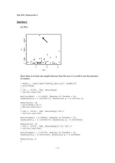
<strong>Since</strong> <strong>there</strong> <strong>is</strong> <strong>at</strong> <strong>least</strong> one sample faraway from the rest, it <strong>is</strong> worth to test the presence<br />
of outliers.<br />
> hm3q1 plot(hm3q1)<br />
><br />
> lm1 outlier.test(lm1)<br />
max|rstudent| = 10.58428, degrees of freedom = 44,<br />
unadjusted p = 1.125766e-13, Bonferroni p = 5.291101e-12<br />
Observ<strong>at</strong>ion: 28<br />
> plot(hm3q1[-28,])<br />
> abline(coef(lm1))<br />
><br />
> lm2 outlier.test(lm2)<br />
max|rstudent| = 4.499644, degrees of freedom = 43,<br />
unadjusted p = 5.113096e-05, Bonferroni p = 0.002352024<br />
Observ<strong>at</strong>ion: 16<br />
> lm3 outlier.test(lm3)<br />
max|rstudent| = 3.907709, degrees of freedom = 42,<br />
unadjusted p = 0.000333085, Bonferroni p = 0.01498882<br />
Observ<strong>at</strong>ion: 6<br />
><br />
- 1 -
<strong>St<strong>at</strong></strong> <strong>849</strong>- <strong>Homework</strong> 3<br />
> lm4 outlier.test(lm4)<br />
max|rstudent| = 2.888445, degrees of freedom = 41,<br />
unadjusted p = 0.006157369, Bonferroni p = 0.2709242<br />
Observ<strong>at</strong>ion: 44<br />
Therefore, we will exclude samples : 6, 16, 28.<br />
(b)<br />
> summary(lm4)<br />
Call:<br />
lm(formula = VL ~ GSS, d<strong>at</strong>a = hm3q1[c(-6, -16, -28), ])<br />
Residuals:<br />
Min 1Q Median 3Q Max<br />
-20544 -12787 -8729 2756 49174<br />
Coefficients:<br />
Estim<strong>at</strong>e Std. Error t value Pr(>|t|)<br />
(Intercept) 11780.0 6900.0 1.707 0.0952 .<br />
GSS 619.2 811.5 0.763 0.4497<br />
---<br />
Signif. codes: 0 ‘***’ 0.001 ‘**’ 0.01 ‘*’ 0.05 ‘.’ 0.1 ‘ ’ 1<br />
Residual standard error: 19460 on 42 degrees of freedom<br />
(1 observ<strong>at</strong>ion deleted due to m<strong>is</strong>singness)<br />
Multiple R-squared: 0.01367, Adjusted R-squared: -0.009813<br />
F-st<strong>at</strong><strong>is</strong>tic: 0.5822 on 1 and 42 DF, p-value: 0.4497<br />
The plot:<br />
> plot(hm3q1[c(-6,-16,-28),1:2])<br />
> abline(coef(lm4))<br />
- 2 -
<strong>St<strong>at</strong></strong> <strong>849</strong>- <strong>Homework</strong> 3<br />
(c) The following figure tells th<strong>at</strong> the normality assumption on error term viol<strong>at</strong>ed as<br />
well. Variance <strong>is</strong> not stable in the first plot, QQ plot shows th<strong>at</strong> it <strong>is</strong> not like normal<br />
d<strong>is</strong>tribution as well.<br />
Residuals vs Fitted<br />
Normal Q-Q<br />
Residuals<br />
-20000 20000<br />
3<br />
21<br />
44<br />
Standardized residuals<br />
-1 0 1 2 3<br />
44 21<br />
3<br />
14000 18000<br />
-2 -1 0 1 2<br />
Fitted values<br />
Theoretical Quantiles<br />
Standardized residuals<br />
0.0 0.5 1.0 1.5<br />
Scale-Loc<strong>at</strong>ion<br />
44 21<br />
3<br />
Standardized residuals<br />
-1 0 1 2 3<br />
Residuals vs Leverage<br />
21 44<br />
Cook's d<strong>is</strong>tance<br />
9<br />
0.5<br />
14000 18000<br />
0.00 0.04 0.08 0.12<br />
Fitted values<br />
Leverage<br />
(d) We can apply Boxcox transform<strong>at</strong>ion.<br />
> par(mfrow=c(1,2))<br />
> b1 lambda hm3q1$y summary(lmb1
<strong>St<strong>at</strong></strong> <strong>849</strong>- <strong>Homework</strong> 3<br />
Coefficients:<br />
Estim<strong>at</strong>e Std. Error t value Pr(>|t|)<br />
(Intercept) 18.43851 2.16262 8.526 5.99e-11 ***<br />
GSS 0.02962 0.24779 0.120 0.905<br />
---<br />
Signif. codes: 0 ‘***’ 0.001 ‘**’ 0.01 ‘*’ 0.05 ‘.’ 0.1 ‘ ’ 1<br />
Residual standard error: 6.302 on 45 degrees of freedom<br />
(1 observ<strong>at</strong>ion deleted due to m<strong>is</strong>singness)<br />
Multiple R-squared: 0.0003173, Adjusted R-squared: -0.0219<br />
F-st<strong>at</strong><strong>is</strong>tic: 0.01428 on 1 and 45 DF, p-value: 0.9054<br />
> plot(hm3q1[,-2])<br />
> abline(coef(lmb1))<br />
> outlier.test(lmb1)<br />
max|rstudent| = 2.707879, degrees of freedom = 44,<br />
unadjusted p = 0.009606887, Bonferroni p = 0.4515237<br />
Observ<strong>at</strong>ion: 28<br />
- 4 -
<strong>St<strong>at</strong></strong> <strong>849</strong>- <strong>Homework</strong> 3<br />
<strong>Question</strong> 2<br />
(a)<br />
4 5 6 7 8 9 10<br />
Brand_Liking<br />
60 70 80 90 100<br />
4 5 6 7 8 9 10<br />
Mo<strong>is</strong>ture_Content<br />
Sweetness<br />
2.0 2.5 3.0 3.5 4.0<br />
60 70 80 90 100 2.0 2.5 3.0 3.5 4.0<br />
From the plot, we can tell Brand_Liking <strong>is</strong> linearly rel<strong>at</strong>ed to Mo<strong>is</strong>ture_Content and<br />
Sweetness.<br />
(b)<br />
> brand fit summary(fit)<br />
Call:<br />
lm(formula = Brand_Liking ~ as.factor(Mo<strong>is</strong>ture_Content) +<br />
as.factor(Sweetness),<br />
d<strong>at</strong>a = brand)<br />
Residuals:<br />
Min 1Q Median 3Q Max<br />
-3.625 -1.312 -0.125 1.563 4.125<br />
Coefficients:<br />
Estim<strong>at</strong>e Std. Error t value Pr(>|t|)<br />
(Intercept) 64.125 1.500 42.737 1.40e-13 ***<br />
as.factor(Mo<strong>is</strong>ture_Content)6 8.000 1.898 4.215 0.00145 **<br />
as.factor(Mo<strong>is</strong>ture_Content)8 19.250 1.898 10.142 6.42e-07 ***<br />
as.factor(Mo<strong>is</strong>ture_Content)10 25.750 1.898 13.567 3.26e-08 ***<br />
as.factor(Sweetness)4 8.750 1.342 6.520 4.31e-05 ***<br />
---<br />
Signif. codes: 0 ‘***’ 0.001 ‘**’ 0.01 ‘*’ 0.05 ‘.’ 0.1 ‘ ’ 1<br />
Residual standard error: 2.684 on 11 degrees of freedom<br />
Multiple R-squared: 0.9597, Adjusted R-squared: 0.9451<br />
- 5 -
<strong>St<strong>at</strong></strong> <strong>849</strong>- <strong>Homework</strong> 3<br />
F-st<strong>at</strong><strong>is</strong>tic: 65.51 on 4 and 11 DF, p-value: 1.338e-07<br />
The coefficients on front of mo<strong>is</strong>ture content {6, 8,10} are the expected differences<br />
between th<strong>at</strong> content and mo<strong>is</strong>ture content 4.<br />
(c)<br />
First plot shows th<strong>at</strong> <strong>there</strong> <strong>is</strong> curve-like rel<strong>at</strong>ion in error terms. It contradicts the<br />
Gauss-Markov assumptions in th<strong>at</strong> error terms are independent.<br />
(d)<br />
- 6 -
<strong>St<strong>at</strong></strong> <strong>849</strong>- <strong>Homework</strong> 3<br />
(e)<br />
The plot in (d) shows th<strong>at</strong> <strong>there</strong> <strong>is</strong> curve-like rel<strong>at</strong>ion. After log transform<strong>at</strong>ion of X1<br />
it looks better from the diagnostic plot below.<br />
> summary(lm2 |t|)<br />
(Intercept) 14.3428 4.6599 3.078 0.00881 **<br />
log(Mo<strong>is</strong>ture_Content) 28.7205 2.1391 13.427 5.37e-09 ***<br />
Sweetness 4.3750 0.7328 5.970 4.67e-05 ***<br />
---<br />
Signif. codes: 0 ‘***’ 0.001 ‘**’ 0.01 ‘*’ 0.05 ‘.’ 0.1 ‘ ’ 1<br />
Residual standard error: 2.931 on 13 degrees of freedom<br />
Multiple R-squared: 0.9432, Adjusted R-squared: 0.9345<br />
F-st<strong>at</strong><strong>is</strong>tic: 108 on 2 and 13 DF, p-value: 7.993e-09<br />
> par(mfrow=c(2,2))<br />
> plot(lm2)<br />
- 7 -
<strong>St<strong>at</strong></strong> <strong>849</strong>- <strong>Homework</strong> 3<br />
Residuals vs Fitted<br />
Normal Q-Q<br />
Residuals<br />
-4 -2 0 2 4<br />
4<br />
7<br />
15<br />
Standardized residuals<br />
-1.0 0.0 1.0 2.0<br />
7<br />
4<br />
15<br />
65 75 85 95<br />
-2 -1 0 1 2<br />
Fitted values<br />
Theoretical Quantiles<br />
Standardized residuals<br />
0.0 0.4 0.8 1.2<br />
Scale-Loc<strong>at</strong>ion<br />
15<br />
4<br />
7<br />
Standardized residuals<br />
-1 0 1 2<br />
Residuals vs Leverage<br />
Cook's d<strong>is</strong>tance<br />
15<br />
4<br />
14<br />
0.5<br />
65 75 85 95<br />
0.00 0.10 0.20<br />
Fitted values<br />
Leverage<br />
(f)<br />
>summary(lm2 |t|)<br />
(Intercept) 14.3428 4.6599 3.078 0.00881 **<br />
log(Mo<strong>is</strong>ture_Content) 28.7205 2.1391 13.427 5.37e-09 ***<br />
Sweetness 4.3750 0.7328 5.970 4.67e-05 ***<br />
---<br />
Signif. codes: 0 ‘***’ 0.001 ‘**’ 0.01 ‘*’ 0.05 ‘.’ 0.1 ‘ ’ 1<br />
- 8 -
<strong>St<strong>at</strong></strong> <strong>849</strong>- <strong>Homework</strong> 3<br />
Residual standard error: 2.931 on 13 degrees of freedom<br />
Multiple R-squared: 0.9432, Adjusted R-squared: 0.9345<br />
F-st<strong>at</strong><strong>is</strong>tic: 108 on 2 and 13 DF, p-value: 7.993e-09<br />
> outlier.test(lm2)<br />
max|rstudent| = 2.055135, degrees of freedom = 12,<br />
unadjusted p = 0.06230417, Bonferroni p = 0.9968668<br />
Observ<strong>at</strong>ion: 15<br />
From outlier test above, we can reject the null hypothes<strong>is</strong> th<strong>at</strong> 15th observ<strong>at</strong>ion <strong>is</strong> an<br />
outlier.<br />
(g)<br />
> plot(leverage)<br />
> abline(h=2*p/n,col='red',lty=1)<br />
> x
<strong>St<strong>at</strong></strong> <strong>849</strong>- <strong>Homework</strong> 3<br />
> (fcv abline(h=fcv,col='red',lty=3)<br />
> ind bigcd fcv)<br />
> text(ind[bigcd],cooks.d<strong>is</strong>tance(lm2)[bigcd]-<br />
0.02,row.names(bp)[bigcd],col='red')<br />
cooks d<strong>is</strong>tance plot<br />
cooks.d<strong>is</strong>tance(lm2)<br />
0.00 0.05 0.10 0.15 0.20 0.25 0.30 0.35<br />
4<br />
7<br />
14<br />
15<br />
5 10 15<br />
Index<br />
So, observ<strong>at</strong>ion 4, 7, 14 and 15 are influential points.<br />
- 10 -
<strong>St<strong>at</strong></strong> <strong>849</strong>- <strong>Homework</strong> 3<br />
<strong>Question</strong> 3<br />
(a)<br />
> hay summary(lm1 |t|)<br />
(Intercept) 2.4750 0.1227 20.177 < 2e-16 ***<br />
as.factor(A)2 2.9750 0.1735 17.150 4.82e-16 ***<br />
as.factor(A)3 3.5000 0.1735 20.176 < 2e-16 ***<br />
as.factor(B)2 2.1250 0.1735 12.250 1.55e-12 ***<br />
as.factor(B)3 2.1000 0.1735 12.106 2.03e-12 ***<br />
as.factor(A)2:as.factor(B)2 1.3500 0.2453 5.503 7.91e-06 ***<br />
as.factor(A)3:as.factor(B)2 2.1750 0.2453 8.866 1.76e-09 ***<br />
as.factor(A)2:as.factor(B)3 1.5750 0.2453 6.420 7.05e-07 ***<br />
as.factor(A)3:as.factor(B)3 5.1750 0.2453 21.094 < 2e-16 ***<br />
---<br />
Signif. codes: 0 ‘***’ 0.001 ‘**’ 0.01 ‘*’ 0.05 ‘.’ 0.1 ‘ ’ 1<br />
Residual standard error: 0.2453 on 27 degrees of freedom<br />
Multiple R-squared: 0.9957, Adjusted R-squared: 0.9944<br />
F-st<strong>at</strong><strong>is</strong>tic: 774.9 on 8 and 27 DF, p-value: < 2.2e-16<br />
> anova(lm1)<br />
Analys<strong>is</strong> of Variance Table<br />
Response: hours<br />
Df Sum Sq Mean Sq F value Pr(>F)<br />
as.factor(A) 2 220.020 110.010 1827.86 < 2.2e-16 ***<br />
as.factor(B) 2 123.660 61.830 1027.33 < 2.2e-16 ***<br />
as.factor(A):as.factor(B) 4 29.425 7.356 122.23 < 2.2e-16 ***<br />
Residuals 27 1.625 0.060<br />
---<br />
Signif. codes: 0 ‘***’ 0.001 ‘**’ 0.01 ‘*’ 0.05 ‘.’ 0.1 ‘ ’ 1<br />
From results above, yˆ23 = 2.475 + 2.975 + 2.100 + 1.575 = 9.125.<br />
(b) Diagnostic plots. Second plot, QQ plot, looks a little skewed, but generally it<br />
looks all right.<br />
- 11 -
<strong>St<strong>at</strong></strong> <strong>849</strong>- <strong>Homework</strong> 3<br />
Residuals vs Fitted<br />
Normal Q-Q<br />
Residuals<br />
-0.4 0.0 0.4<br />
6<br />
23<br />
29<br />
Standardized residuals<br />
-2 -1 0 1 2<br />
23 629<br />
4 6 8 10 12<br />
-2 -1 0 1 2<br />
Fitted values<br />
Theoretical Quantiles<br />
Standardized residuals<br />
0.0 0.4 0.8 1.2<br />
Scale-Loc<strong>at</strong>ion<br />
6<br />
23<br />
29<br />
4 6 8 10 12<br />
Standardized residuals<br />
-2 -1 0 1 2<br />
Constant Leverage:<br />
Residuals vs Factor Levels<br />
6<br />
23<br />
29<br />
as.factor(A) :<br />
1 2 3<br />
Fitted values<br />
Factor Level Combin<strong>at</strong>ions<br />
(c) There <strong>is</strong> some interaction since they are not always parallel.<br />
B<br />
hours<br />
4 6 8 10 12<br />
3<br />
2<br />
1<br />
1 2 3<br />
A<br />
- 12 -
<strong>St<strong>at</strong></strong> <strong>849</strong>- <strong>Homework</strong> 3<br />
(d)<br />
From the result of ANOVA above, we can see th<strong>at</strong> F st<strong>at</strong><strong>is</strong>tic <strong>is</strong> 122.23. So we reject<br />
null hypothes<strong>is</strong> th<strong>at</strong> <strong>there</strong> <strong>is</strong> no interaction.<br />
(e)<br />
F st<strong>at</strong><strong>is</strong>tic <strong>is</strong> 18827.86 for A and 1027.33 for B. So we reject null hypothes<strong>is</strong> th<strong>at</strong> <strong>there</strong><br />
<strong>is</strong> no main effect.<br />
<strong>Question</strong> 4<br />
ˆ ε = Y − Yˆ<br />
= ( I − H ) Y , and H and ( I − H ) <strong>is</strong> idempotent.<br />
(a) E ( ˆ) ε = E(<br />
Y −Yˆ)<br />
= Xβ<br />
− Xβ<br />
= 0<br />
2<br />
2 2<br />
(b) cov( ˆ) ε = cov(( I − H ) Y ) = σ ( I − H ) = σ ( I − H )<br />
2<br />
2<br />
(c) cov( ˆ, ε Y ) = cov( Y −Yˆ,<br />
Y ) = ( I − H ) cov( Y ) = σ ( I − H )<br />
(d) cov( ˆ, ε Yˆ)<br />
= cov(( I − H ) Y,<br />
HY)<br />
= ( I − H )cov( Y ) H = cov( Y )( I − H ) H = 0<br />
(e) ˆ<br />
−1<br />
X ' ˆ ε = X '( Y − X ˆ) β = X ' Y − X ' Xβ<br />
= X ' Y − X ' X ( X ' X ) X ' Y = X ' Y − X ' Y = 0<br />
p×<br />
1<br />
n<br />
n<br />
1<br />
ˆε <strong>is</strong> the first row of X ' εˆ because the first row <strong>is</strong> 1 vector. Therefore ˆ ε = 0<br />
∑<br />
i=<br />
1<br />
i<br />
(f) ˆ ε ' Y = (( I − H ) Y )' Y = Y '( I − H ) Y because ( I − H ) <strong>is</strong> symmetric.<br />
(g) ˆ ε ' Yˆ<br />
= (( I − H ) Y )' Yˆ<br />
= Y '( I − H ) HY = 0<br />
(h)<br />
ˆ' ε X = (( I − H ) Y )' X = Y '( I − H ) X = Y ' X −Y<br />
' HX<br />
−1<br />
= Y ' X −Y<br />
' X ( X ' X ) X ' X = Y ' X −Y<br />
' X = 0<br />
n<br />
∑<br />
i=<br />
1<br />
i<br />
- 13 -
<strong>St<strong>at</strong></strong> <strong>849</strong>- <strong>Homework</strong> 3<br />
<strong>Question</strong> 5<br />
(a)<br />
X<br />
*<br />
' X<br />
∑<br />
n<br />
⎡<br />
2<br />
1 ( X − )<br />
= 1 1<br />
X<br />
i i 1<br />
⎢<br />
⎢ n −1<br />
SX1<br />
* SX1<br />
=<br />
⎢<br />
n<br />
− −<br />
⎢ 1 ∑ ( X )(<br />
= 1<br />
X1<br />
X<br />
2<br />
X<br />
i i<br />
i<br />
⎢⎣<br />
n −1<br />
SX1<br />
* SX<br />
2<br />
1 2<br />
)<br />
∑<br />
n<br />
1 ( X − −<br />
= 1<br />
X<br />
1)(<br />
X<br />
2<br />
X<br />
i i<br />
i<br />
n −1<br />
SX1<br />
* SX<br />
2<br />
n<br />
2<br />
1 ∑ ( X − )<br />
= 1 2<br />
X<br />
i i 2<br />
n −1<br />
SX * SX<br />
1 2<br />
2<br />
2<br />
) ⎤<br />
⎥<br />
⎥ ⎡1<br />
⎥<br />
= ⎢<br />
⎥<br />
⎣r<br />
⎥⎦<br />
r⎤<br />
1<br />
⎥<br />
⎦<br />
Therefore,<br />
* * −1<br />
2<br />
2 2<br />
2 2<br />
Var ( β ) = ( X ' X ) σ * . Then we will have σ<br />
β 1*<br />
= σ<br />
β 2*<br />
= σ * /(1 − r )<br />
(b) When the intercorrel<strong>at</strong>ions among the predictor variables increase, it will increase<br />
the variance of the estim<strong>at</strong>es.<br />
- 14 -
<strong>St<strong>at</strong></strong> <strong>849</strong>- <strong>Homework</strong> 3<br />
<strong>Question</strong> 6<br />
(a)<br />
⎡1<br />
0 0 1 0 0⎤<br />
⎢<br />
⎥<br />
⎢<br />
1 0 0 0 1 0<br />
⎥<br />
⎢0<br />
1 0 1 0 0⎥<br />
X = ⎢<br />
⎥ , rank(X) =5<br />
⎢0<br />
1 0 0 0 1⎥<br />
⎢0<br />
0 1 0 1 0⎥<br />
⎢<br />
⎥<br />
⎣0<br />
0 1 0 0 1<br />
⎦<br />
(b) Here I will first show why β<br />
1<br />
<strong>is</strong> not estimable.<br />
Suppose we can estim<strong>at</strong>e β<br />
1<br />
, then we should have a vector C such th<strong>at</strong><br />
⎧ c1<br />
+ c2<br />
= 1<br />
⎪<br />
⎪<br />
c3<br />
+ c4<br />
= 0<br />
⎪c5<br />
+ c6<br />
= 0<br />
CX = (1,0,0,0,0,0) . Then we will have ⎨ . Th<strong>is</strong> system has no solution.<br />
⎪c1<br />
+ c3<br />
= 0<br />
⎪c2<br />
+ c5<br />
= 0<br />
⎪<br />
⎩c4<br />
+ c6<br />
= 0<br />
Therefore a<br />
1<br />
<strong>is</strong> not estimable. Similarly the rest components of β <strong>is</strong> not estimable.<br />
(c) Let CX = ( 1, −1,0,0,0,0<br />
) , we will have<br />
⎧ c1<br />
+ c2<br />
= 1<br />
⎪<br />
⎪<br />
c3<br />
+ c4<br />
= −1<br />
⎪ c5<br />
+ c6<br />
= 0<br />
⎨ . We can set C=(1,0,-1,0,0,0). Therefore ψ<br />
1<br />
<strong>is</strong> estimable.<br />
⎪ c1<br />
+ c3<br />
= 0<br />
⎪ c2<br />
+ c5<br />
= 0<br />
⎪<br />
⎩ c4<br />
+ c6<br />
= 0<br />
Let CX = ( 1,1, −2,0,0,0)<br />
, we will have<br />
⎧ c1<br />
+ c2<br />
= 1<br />
⎪<br />
⎪<br />
c3<br />
+ c4<br />
= 1<br />
⎪c5<br />
+ c6<br />
= −2<br />
⎨ . We can set C=(0,1,0,1,-1,-1). Therefore ψ<br />
2<br />
<strong>is</strong> estimable.<br />
⎪ c1<br />
+ c3<br />
= 0<br />
⎪ c2<br />
+ c5<br />
= 0<br />
⎪<br />
⎩ c4<br />
+ c6<br />
= 0<br />
- 15 -


