Wheeler, Mechanics

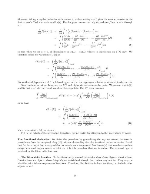
Moreover, taking a regular derivative with respect to α then setting α = 0 gives the same expression as the
first term of a Taylor series in small h(x). This happens because the only dependence f has on α is through
x :
d
d
f [x(λ, α)] =
dα dα
=
=
∫
(
)
L x (λ, α) , x (1) (λ, α) , . . . dλ
∫ ( ∂L ∂x
∂x ∂α +
∫ ( ∂L
∂x h +
∂L ∂x (1)
∂x (1) ∂α + . . . + ∂L ∂x (n) )
dλ (8)
∂x (n) ∂α
∂L
∂x (1) h(1) + . . . +
∂L )
∂x (n) h(n) dλ (9)
so that when we set α = 0, all dependence on x (λ) + αh (λ) reduces to dependence on x (λ) only.
therefore define the variation of f [x] as
We
δf [x (λ)]
≡
=
=
( )∣ d
∣∣∣α=0
dα f [x(λ, α)]
∫ ( ∂L (x (λ, α))
h + . . . +
∂x
∫ ( ∂L (x (λ))
h +
∂x
)∣
∂L (x (λ, α)) ∣∣∣α=0
h (n) dλ
∂x (n)
)
∂L (x (λ))
h (1) ∂L (x (λ))
+ . . . + h n dλ
∂x (1)
∂x (n)
Notice that all dependence of L on h has dropped out, so the expression is linear in h (λ) and its derivatives.
Now continue as before. Integrate the h (1) and higher derivative terms by parts. We assume that h (λ)
and its first n − 1 derivatives all vanish at the endpoints. The k th term becomes
∫ 1
∣ ∫ (
∂L ∣∣∣x(λ,α)=x(λ) 1
∣ )
h (k) (λ) dλ = (−1) k dλ dk ∂L ∣∣∣x=x(λ)
∂x (k) dλ k h (λ)
∂x (k)
so we have
0
0
δf [x (λ)] =
=
( )∣ d
∣∣∣α=0
dα f [x(λ, α)]
∫ 1
( ∂L (x (λ))
− d ∂L (x (λ))
0 ∂x dλ ∂x (1)
+ . . . + (−1) n d n
)
∂L (x (λ))
dλ n h (λ) dλ (10)
∂x (n)
where now, h (λ) is fully arbitrary.
Fill in the details of the preceeding derivation, paying particular attention to the integrations by parts.
The functional derivative We finish the procedure by generalizing the way we extract the term in
parentheses from the integrand of eq.(10), without demanding that the functional derivative vanish. Recall
that for the straight line, we argued that we can choose a sequence of functions h(x) that vanish everywhere
except in a small region around a point x 0 . It is this procedure that we formalize. The required rigor is
provided by the Dirac delta function.
The Dirac delta function To do this correctly, we need yet another class of new objects: distributions.
Distributions are objects whose integrals are wel-defined though their values may not be. They may be
identified with infinite sequences of functions. Therefore, distributions include functions, but include other
objects as well.
26