Analysis of Nominal and Ordinal Data (pdf)

Analysis of Nominal
and Ordinal Data
•Construction and Analysis of
Contingency Tables
•Statistical Aids for Interpretation
•Control Table Analysis
•Aaron D. Schroeder, PhD

Construction and Analysis
of Contingency Tables
• We have previously discussed levels of
measurement (nominal, ordinal, interval),
and the measures of central tendency
and dispersion that can be used to
summarize a group of data – This was
single variable or “univariate” statistics
• This type of analysis is common, but
generally reflects the first step in the
analysis of a problem

• Imagine you work in the Public Affairs
department of a large state agency
• Just finished annual survey of public opinion
toward the agency
• Initial results show most people feel agency is
doing a “very poor job” with a median of “poor
job”
• This is a dramatic downturn from previous
years
• Now that you have done the descriptive,
univariate statistics, what do you do?

• You DON‟T want to give this information to the agency
director without some idea of how the public image of
the agency might be improved
• You need to consider WHY public support has fallen
• Perhaps program cuts hit a particularly populous
county harder than others
• Perhaps the new director has a bad reputation “Mean”
Gean Maculroy they call him
• Either explanation would result in completely different
approaches to improving the public image of the
agency
• In both, we want to know the “relationship” between
TWO variables (county and opinion, view of director
and opinion)

• The method that is most employed to
quickly analyze the relationship between
two variables is called Contingency Table
Analysis or the analysis of Crosstabulations
(Cross-tabs)
• Here we will learn hw to construct crosstabs
and interrupter them

Percentage Distributions
• First, though, we will review percentage
distributions, as they are integral to crosstabulations
• As we have explored before, a percentage
distribution is simply a frequency distribution
that has been converted to percentages
• It tabulates the percentage associated with
each data value or group (class) of data values

Percentage Distributions
• Consider this table of
responses to whether or
not there are “too many”
bureaucrats in the
federal government
• Mode is “Agree”, but still
difficult to interpret
• Percentages would
make it easier to
interpret and compare to
previous years
Response
Strongly Agree 686
Agree 979
Neutral 208
Disagree 436
Strongly
Disagree
Number of
People
232
2,541

Steps in Percentaging
• The steps for Percentaging are easy:
• 1. Add the number of people (frequencies)
giving each of the responses. In our table that‟s
686+979+208+436+232=2,541
• 2. Divide each of the individual frequencies by
this total and multiply the result by 100. For
“Strongly Agree” we divide 686 by 2,541, then
multiply by 100 = 26.997
• So, about 27.0 percent responded “Strongly
Agree”

Displaying and Interpreting
Percentage Distributions
• It is clear from this
distribution that most
respondents “Agree”
with the statement
and that the extent of
“general agreement”
far outweighs the
extent of “general
disagreement”
Response
Strongly Agree 27.0
Agree 38.5
Neutral 8.2
Disagree 17.2
Strongly
Disagree
Percentage
9.1
Total 100.0
N = 2,541

Collapsing Percentage
Distributions
Response
Strongly Agree or Agree 65.5
Neutral 8.2
Disagree or Strongly Disagree 26.3
Total 100.0
Percentage
N = 2,541
• It is perfectly ok to collapse percentage distributions as long as the
categories are close in substantive meaning (e.g. you can‟t include
Neutral with either collapsed category
• The only time you can violate that rule is when dealing with nominal
variables where there are many categories with little data (e.g.
Protestant 62%, Catholic 22%, Jewish 13%, Other 3%)

In-Class Task
• Construct a
collapsed
percentage
distribution of
the data here
• How would
you collapse
it?
• One will
present
Where do people shop?
Main Store Named (and location)
Cleo‟s (neighborhood store) 5
Morgan‟s (downtown) 18
Wiese‟s (eastern shopping center) 12
Cheatham‟s (neighborhood store) 2
Shop City (eastern shopping center) 19
Food-o-Rama (western shopping center) 15
Stermer‟s (downtown) 7
Binzer‟s (neighborhood store) 2
England‟s (western shopping center) 1
Bargainville‟s (eastern shopping center) 26
Whiskey River (downtown) 13
Number of
Persons
120

Contingency Table
Analysis
• A “univariate” frequency distribution
simply presents the number of cases (or
frequency) taking each value of a given
variable
• A “bivariate” frequency distribution
presents the number of cases that fall
into each possible pairing of the values or
categories of two variables
simultaneously

Constructing Contingency
Tables
• Consider the
variables “race” and
“gender” for
volunteers to the
Klondike
Expessionist Art
Museum
• There are four
possible pairings
“Gender”
Female
Male
“Race”
White
Nonwhite

Constructing Contingency
Tables
• The cross-tabulation of
these two variables
displays the number of
cases (volunteers) that
fall into each of the racegender
combinations
• Called a “crosstabulation”
precisely
because it it crosses
(and tabulates) each of
the categories of one
variable with each of the
categories of a second
variable
Race and Gender of Volunteers to
Klondike Expressionist Art Museum
Race
Sex White Nonwhite Total
Male 142 109 251
Female 67 133 200
Total 209 242 451

Terminology
• Cell
• The cross-classification of
one category each from
two variables
• Marginals
• The totals of each column
and the totals for each row
• Grand Total
• The total number of cases
represented in the table
(N)
Race and Gender of Volunteers to
Klondike Expressionist Art Museum
Race
Sex White Nonwhite Total
Male 142 109 251
Female 67 133 200
Total 209 242 451

In-Class Task
• Create a cross-tabulation called “Relationship
between Type of Employment and Attitude
toward Balancing the Federal Budget”
• The variables of interest are “type of
employment” (public, private, nonprofit) and
“attitude toward balancing the federal budget”
(approve, disapprove)
• The cell frequencies are: public-disapprove 126;
public-approve 54; private-disapprove 51;
private-approve 97; nonprofit-disapprove 25;
nonprofit-approve 38

Relationships Between
Variables
• Managers make and analyze cross-tabs
because they are interested in the relationship
between two variables
• A statistical relationship is a recognizable
change in one variable as the other variable
changes
• The cell frequencies of a cross-tabulation
provide some information regarding whether
changes in one variable are statistically related
to changes in another

Relationships Between
Variables
Relationship between Educational Level and
Performance on Civil Service Examination
Performance
on Civil Service
Examination
High School or
Less
Education
More Than High
School
Total
Low 100 200 300
High 150 800 950
Total 250 1,000 1,250

Analysis Process
• Step 1 – Determine which variable is
Independent and which is Dependent
• Independent variable – the anticipated
causal variable – the one that leads to
changes or effects in the other variable
• Dependent variable – the one that gets
influenced

Analysis Process
• Stated as a Hypothesis: the higher the
education, the higher the expected score
on the test
• So, education is the independent variable
and performance on the test is the
dependent variable

Analysis Process
• Step 2 – Calculate percentages within the
categories of the independent variable
• In this case, education
• We would like to know the percentage of
people with high school education or less (low
education) who received high scores on the
exam and the percentage of people with more
than a high school education (high education)
who received high scores
• We could then compare and test our
hypothesis

• Go ahead and calculate the percentages within the
categories of the independent variable
Relationship between Educational Level and Performance
on Civil Service Examination
Performance
on Civil
Service
Examination
High School or
Less
Education
More Than
High School
Total
Low 100 200 300
High 150 800 950
Total 250 1,000 1,250

Analysis Process
• Step 3 – Compare the percentages calculated
within the categories of the independent
variable for one of the categories of the
dependent variable
• For example, whereas 80% of those with high
education earned high scores on the civil
service examination, only 60% of those with
low education did so.
• Therefore, our hypothesis is supported by
these data

Analysis Process
• Step 4 (optional) – Calculate a percentage
difference across one of the categories of the
dependent variable
• Not usually included in the table, but in the
write-up discussing support for the hypothesis
• A percentage difference is a measure
of the strength of the relationship
between the two variables

In-Class Task
• Automobile Maintenance in Berrysville
handout

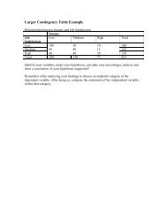
Larger Contingency
Tables
• In cross-tabs larger than 2 x 2 analysis is
conducted using the same process
• However, the choice of which category of
the Dependent Variable is selected for
analysis requires more care (it doesn‟t
matter in a 2x2 table)
• Avoid intermediate categories – choose an
endpoint category – choose “low” or “high”
in a “low”, “medium”, “high” variable
• Do the same for the Independent Variable

In-Class Task
• Relationship between Income and Job
Satisfaction handout

Hypothesis 1: The higher the income, the higher the job satisfaction
Hypothesis 2 (corollary): The lower the income, the lower the job satisfaction

Which one should you use?
• Since they both confirm your hypothesis, but to
a different degree, report BOTH.
• Income appears to make a difference of 37%
to 47% in job satisfaction.
• What if the two disagree?
• Then you really can‟t draw a conclusion. The
problem is more complex than you thought and
you‟ll have to revisit what you thought the
relationship was and how you have phrased
the question.

Displaying Contingency
Tables
• Conventions for the display of contingency tables or
cross-tabs
• Don‟t show the raw frequencies – just show the percentages
• The independent variable is placed along the columns of the
table
• The dependent variable is positioned down the rows of the
table
• The independent variable (if ordinal) should progress from left
to right (least to most)
• The dependent variable (if ordinal) should progress from top to
bottom (least to most)
• The percentages calculated within the categories of the
independent variable are summed down the column with a
total at the foot of the respective column
• The total number of cases (n=) is listed below the total
percentage for each column

Conventional Format for a
Contingency Table
Dependent
Variable
Substantive
meaning of
categories
increases
Independent Variable
Substantive meaning of categories increases (e.g., “low,” “medium,” “high”)
_____% _____% _____% _____%
_____% _____% _____% _____%
_____% _____% _____% _____%
Total 100.0% 100.0% 100.0% 100.0%
(n = ___ ) (n = ___ ) (n = ___ ) (n = ___ )

Computer Printouts
• Be careful with computer contingency tables
(like excel)
• The “wizards” can give three different
percentages
• Columns
• Rows
• Percentage of Total Table
• It doesn‟t know any better – you need to know
better!

In-Class Problems
• Teams of 2
• Prepare and present

Question 1
• The Lebanon postmaster suspects that working on
ziptronic machines is the cause of high absenteeism.
More than 10 absences from work without businessrelated
reasons is considered excessive absenteeism.
A check of employee records shows that 26 of the 44
ziptronic operators had 10 or more absences and 35 of
120 non-ziptronic workers had 10 or more absences.
Construct a contingency table for the postmaster. Does
the table support the postmaster‟s suspicion that
working on ziptronic machines is related to high
absenteeism?

Question 2
The Egyptian Air Force brass believe that overweight pilots have slow
reaction times. They attribute the poor performance of their air force in
recent war games in the Sinai to overweight pilots. The accompanying
data were collected for all pilots. Analyze these data for the Egyptian Air
Force.
Pilot Weight
Reaction
Time
Normal Up to 10
Pounds
Overweight
Poor 14 36 45
Adequate 35 40 33
Excellent 46 25 15
More than
10 Pounds
Overweight

Question 3
The state personnel office oversees the state‟s tuition assistance program,
which pays the tuition of civil servants taking courses for an MPA. Only two
schools offer an MPA degree in the state capital, Capital College of Law and
East Winslow State University. Some concern is expressed by legislators that
many tuition-assisted students do not graduate. Analyze the data in the
accompanying table for the personnel office.
Students Assisted for MPA Tuition
Status Capital East Winslow
Did not graduate 69 83
Graduated 23 37

Question 4
As head scheduler of special events for the Incomparable
Myriad (the city arena), your task is to schedule events
that make a profit so that the city need not subsidize the
arena. Analyze the data in the accompanying table, which
is based on last year‟s data, and report to the city council.
Type of Event
Status Hockey Games Religious
Rallies
Not
Profitable
Basketball
Games
Rock Concerts
24 4 21 2 3
Profitable 18 32 6 8 0
Public
Administration
Conventions

Question 5
The Cancer Institute is evaluating an experimental drug for
controlling lip cancer. Eighty lip cancer victims are
randomly selected and given the drug for 1 year. Sixty
other lip cancer victims are randomly selected and given a
placebo for a year. From the data in the accompanying
table, what would you conclude?
Cancer Status Drug Group Placebo Group
Active 58 42
Remission 22 18

Question 6
A professor of public administration has kept records on the class
participation of his students over the past several years. He has a
strong feeling (hypothesis) that class participation is related to grade in
the course. For this analysis he classifies course grades into two
categories, fail and pass. He operationalizes class participation as “low”
if the student participated in class discussion in fewer than 25% of class
periods, and “high” if the student participated in 25% or more of the
periods. Based on these definitions, he has assembled the crosstabulation
below. Does a relationship exist between class participation
and course grades?
Class Participation
Grade in Course Low High
Fail 56 15
Pass 178 107

Question 7
Madonna Lewis‟s job in the Department of Sanitary Engineering is to
determine whether new refuse collection procedures have improved
the public‟s perception of the department. Public opinion surveys
were taken both before and after the new procedures were
implemented. The results appear in the accompanying table.
Analyze the table, and evaluate whether public perception of the
department appears to have improved over time.
Opinion Before After
Department is
doing a poor job
Department is
doing a good
job
79 73
23 47

BREAK

Statistical Aids for
Interpretation
• So we now know how to determine if two
nominal or ordinal variables are related
statistically using a contingency table and
percentages
• But now we have to ask, “How strong” is that
relationship?
• Can we say that the relationship is “strong
enough” to have not occurred by chance?

Chi-Square Test: Statistical
Significance for Contingency Tables
• A procedure for evaluating the level of statistical
significance attained by a bivariate relationship in a
cross-tabulation
• Statistical Significance – how confident can we be that
this sample of data represents its parent population?
(We will get into this in more detail next week, but this
definition is sufficient for now)
• Chi Square – assumes there is “no relationship”
between the two variables and determines if the
relationship you think you are seeing is possibly just do
to chance

Chi Square – 3 Steps
• First – you calculate “expected frequencies” for
each cell in your contingency table – what
would be there if the was “no” relationship
• Second – you calculate the difference between
these expected frequencies and the actual
frequencies – this is Chi Square
• Third – you look up the value in a table to
determine the degree of confidence that a
relationship exists

Chi-Square Example – Step
By Step
• A disgruntled official working in the personnel
department of a large federal bureaucracy is
disturbed by the level of incompetence she
perceives in the leadership of the organization.
• She is convinced that incompetence rises to
the top
• She shares this thought with a coworker who
challenges her to substantiate her claim

Chi-Square Example – Step
By Step
• So, ignoring all personnel law, she selects a
random sample of 400 people employed by the
organization
• Using their civil service exams, she classifies
them into three levels of competence (low,
medium, high)
• Using their job descriptions, she classifies
them into three levels of hierarchical position
(low, medium, high)

Chi-Square Example – Step
By Step
Cross-Tabulation of Competence and Hierarchy
Competence
Hierarchy Low Medium High Total
Low 113 60 27 200
Medium 31 91 38 160
High 8 8 24 40
Total 152 159 89 400

Chi-Square : Step 1
• Compute the expected frequencies for each
cell assuming no relationship between the
independent and dependent variables (need to
be working with actual frequencies, not
percentages)
• For no relationship, we would expect there to
be identical distributions of the dependent
variable for each value of the independent
variable
• For each level of “Competence” (low, medium,
high), the distribution o hierarchy (low,
medium, high) should be the same

No Relationship would
look like this
Hypothetical No-Relationship Cross-Tabulation for Chi-Square
Competence
Hierarchy Low Medium High Total
Low 50% 50% 50% 50%
(n=200)
Medium 40% 40% 40% 40%
(n=160)
High 10% 10% 10% 10% (n=40)
The proportion for each value of the Hierarchy would be the same for each
Level of Competence (e.g. if the total proportion of “low in the hierarchy”
Is 50%, then it would be 50% for each value of competence

Chi-Square : Step 1
• Calculating the expected
frequencies is
cumbersome but easy
• Multiply the total
proportional percentage
of a value of the
dependent variable (e.g.
low in the hierarchy is
50%) by the total for
each value of the
independent variable
(e.g. 152 for low
competence)
Cross-Tabulation of Competence and
Hierarchy
Competence
Hierarchy Low Med High Total
Low .50 x 152 =
76.0
200
(50%)
Medium 160
(40%)
High 40
(10%)
Total 152 159 189 400
(100%)

Chi-Square : Step 1
Calculations for Expected Frequencies
Table Cell
Competence Hierarchy Observed Expected
Low Low 113 .50x152=76.0
Low Medium 31 .40x152=60.8
Low High 8 .10x152=15.2
Medium Low 60 .50x159=79.5
Medium Medium 91 .40x159=63.6
Medium High 8 .10x159=15.9
High Low 27 .50x89=44.5
High Medium 38 .40x89=35.6
High High 24 .10x89=8.9
Total 400 400

Chi-Square : Step 2
• Compute the value of Chi-Square
• Find out what the difference is between
each observed frequency and what
would be expected if no relationship
• Square that difference
• Divide that by the expected frequency
• Add them all up, and, voila, you‟ve got
chi-square!

Chi-Square : Step 2
Calculations for Expected Frequencies
Table Cell
Competence Hierarchy Observed Expected (O-E) 2 /E
Low Low 113 .50x152=76.0 18.01
Low Medium 31 .40x152=60.8 14.61
Low High 8 .10x152=15.2 3.41
Medium Low 60 .50x159=79.5 4.78
Medium Medium 91 .40x159=63.6 11.8
Medium High 8 .10x159=15.9 3.93
High Low 27 .50x89=44.5 6.88
High Medium 38 .40x89=35.6 .16
High High 24 .10x89=8.9 25.62
Total 400 400 89.2
CHI-SQUARE!

Chi-Square : Step 3
• Figure out the degrees of freedom and
statistical significance level
• Degrees of freedom: How big is your table? Multiply
number of rows -1 by number of columns – 1; so,
(3-1)x(3-1)=4
• Statistical significance level: probability your „wrong‟
– chance you‟re willing to put up with
(conventionally set at 5%)
• Look it up!
• Back of any stats or methods book, Chi-Square
distribution table (4 df down the side, .05 across the
top)

Chi-Square : Step 3
• What value do you get?
• If your chi-square value is higher than that,
then you‟ve found a relationship that is
statistically significant!
• So, is there a relationship between
Competence and Hierarchy?
• Is her hypothesis correct?
• In class – percentage the table and evaluate

Limitations of Chi-Square
• Chi-square helps you determine if a
relationship exists (is statistically
significant)
• Chi-square does not tell you how
strong that relationship is or which
direction that relationship takes
(positive, negative, etc.)

Assessing the Strength of a
Relationship: Percentage Difference
• The easiest and most
common method for
assessing the strength
and direction of a
relationship is to simply
use the percentage
distribution!
• Do this BEFORE trying
any fancier statistics!
• The closer you are to a
perfect positive or
negative relationship,
the stronger the
relationship!
Perfect Positive Relationship
Dependent
Variable
Independent Variable
Category 1 Category 2
Category 1 100% 0%
Category 2 0% 100%
100% 100%

In-Class Task
• Figure chi-square for this
table as well as
percentaging it
• Is there a statistically
significant relationship
there at the 5% level;
what about the 10%
level?
• Looking at the
percentages, can you
state the relationship in
“directional” language?
Capital
Punishment
Percent in
Favor
Percent
Opposed
Liberal Conservative
25 52
37 43

Measures of Association
• What if you can‟t really tell how strong the relationship
is, or in what direction?
• Like if you have a very large table?
• That‟s when you use “measures of association” –
fancier stats
• Cramer‟s V, lambda, Gamma, Somer‟s d, and others
• They give you a number that you can tell the strength
and direction (if ordinal or interval) of a relationship
• If stat made for Nominal data (e.g. Cramer‟s V), then
the number will be between 0 and 1 (e.g. .49)
• If made for ordinal/interval, then will usually be
between -1 and 1 to give both strength and direction.

A Common Measure:
Cramer’s V
• While you will generally not run across
many measures of association in your
work, if you d, it will most likely be
Cramer‟s V
• Non-directional between 0-1

Statistical Control Table
Analysis
• According to
this percentage
distribution,
does Ice Cream
Consumption
influence the
rate of juvenile
crime?
• What might be
going on?
Relationship between Juvenile Crime and Ice
Cream Consumption
Ice Cream Consumption
Crime rate Low High
Low 25% 80%
High 75% 20%
Total 100% 100%
(n = 20
precincts)
(n = 25
precincts)

Controlling for a Third
Variable
SES
Ice Cream
Consumption
?
Juvenile Crime

Controlling for a Third
Variable
• How we control for a third variable is
deceptively simple
• You just examine the relationship
between the original two variables within
each of the categories of the control
variable, then compare results across the
categories of the control
• Sounds more difficult than it is

Example: Alcoholism
• Handout

In-Class Task
• General Halftrack
suspects that
Colonel Sy Verleaf is
discriminating in his
promotions by
promoting more
whites than nonwhites.
The table
illustrates this
hypothesis.
Status
Passed
Over
Promote
d
Race
Nonwhite
White
Total
23 14 37
27 86 113
Total 50 100 150

In-Class Task
• When called in to
explain, Colonel
Verleaf presents the
following tables in his
defense
Non-West Pointers‟ Race
Status Non-white White
Passed
Over
20 12
Promoted 19 12
West Pointers‟ Race
Status Non-white White
Passed
Over
3 2
Promoted 8 74

Status
Passed
Over
Promote
d
Race
Nonwhite
White
Total
23 14 37
27 86 113
Total 50 100 150
Percentage the Tables
What does the first table seem to
show?
What variable is Colonel Verleaf
trying to control for?
What would be your report to
General Halftrack about Colonel
Verleaf?
Non-West Pointers‟ Race
Status Non-white White
Passed
Over
20 12
Promoted 19 12
West Pointers‟ Race
Status Non-white White
Passed
Over
3 2
Promoted 8 74

Quiz