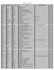
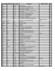
Download - Susquehanna University

Surface Evolver Manual 

Version 2.30 

January 1, 2008 

Kenneth A. Brakke 

Mathematics Department 

Susquehanna University 

Selinsgrove, PA 17870 

brakke@susqu.edu 

http://www.susqu.edu/brakke

Contents 

1 Introduction. 9 

1.1 General description . . . . . . . . . . . . . . . . . . . . . . . . . . . . . . . . . . . . . . . . . . . . 9 

1.2 Portability . . . . . . . . . . . . . . . . . . . . . . . . . . . . . . . . . . . . . . . . . . . . . . . . . 9 

1.3 Bug reports . . . . . . . . . . . . . . . . . . . . . . . . . . . . . . . . . . . . . . . . . . . . . . . . 10 

1.4 Web home page . . . . . . . . . . . . . . . . . . . . . . . . . . . . . . . . . . . . . . . . . . . . . . 10 

1.5 Newsletter . . . . . . . . . . . . . . . . . . . . . . . . . . . . . . . . . . . . . . . . . . . . . . . . . 11 

1.6 Acknowledgements . . . . . . . . . . . . . . . . . . . . . . . . . . . . . . . . . . . . . . . . . . . . 11 

2 Installation. 12 

2.1 Microsoft Windows . . . . . . . . . . . . . . . . . . . . . . . . . . . . . . . . . . . . . . . . . . . . 12 

2.2 Macintosh . . . . . . . . . . . . . . . . . . . . . . . . . . . . . . . . . . . . . . . . . . . . . . . . . 13 

2.3 Unix/Linux . . . . . . . . . . . . . . . . . . . . . . . . . . . . . . . . . . . . . . . . . . . . . . . . 13 

2.3.1 Compiling . . . . . . . . . . . . . . . . . . . . . . . . . . . . . . . . . . . . . . . . . . . . 14 

2.4 Geomview graphics . . . . . . . . . . . . . . . . . . . . . . . . . . . . . . . . . . . . . . . . . . . . 14 

2.5 X-Windows graphics . . . . . . . . . . . . . . . . . . . . . . . . . . . . . . . . . . . . . . . . . . . 15 

3 Tutorial 16 

3.1 Basic Concepts . . . . . . . . . . . . . . . . . . . . . . . . . . . . . . . . . . . . . . . . . . . . . . 16 

3.2 Example 1. Cube evolving into a sphere . . . . . . . . . . . . . . . . . . . . . . . . . . . . . . . . . 17 

3.3 Example 2. Mound with gravity . . . . . . . . . . . . . . . . . . . . . . . . . . . . . . . . . . . . . 20 

3.4 Example 3. Catenoid . . . . . . . . . . . . . . . . . . . . . . . . . . . . . . . . . . . . . . . . . . . 22 

3.5 Example 4. Torus partitioned into two cells . . . . . . . . . . . . . . . . . . . . . . . . . . . . . . . 24 

3.6 Example 5. Ring around rotating rod . . . . . . . . . . . . . . . . . . . . . . . . . . . . . . . . . . . 26 

3.7 Example 6. Column of liquid solder . . . . . . . . . . . . . . . . . . . . . . . . . . . . . . . . . . . 31 

3.8 Example 7. Rocket fuel tank . . . . . . . . . . . . . . . . . . . . . . . . . . . . . . . . . . . . . . . 34 

3.8.1 Surface energy . . . . . . . . . . . . . . . . . . . . . . . . . . . . . . . . . . . . . . . . . . 34 

3.8.2 Volume . . . . . . . . . . . . . . . . . . . . . . . . . . . . . . . . . . . . . . . . . . . . . . 35 

3.8.3 Gravity . . . . . . . . . . . . . . . . . . . . . . . . . . . . . . . . . . . . . . . . . . . . . . 36 

3.8.4 Running . . . . . . . . . . . . . . . . . . . . . . . . . . . . . . . . . . . . . . . . . . . . . . 37 

3.9 Example 8. Spherical tank . . . . . . . . . . . . . . . . . . . . . . . . . . . . . . . . . . . . . . . . 39 

3.9.1 Surface energy . . . . . . . . . . . . . . . . . . . . . . . . . . . . . . . . . . . . . . . . . . 40 

3.9.2 Volume . . . . . . . . . . . . . . . . . . . . . . . . . . . . . . . . . . . . . . . . . . . . . . 41 

3.9.3 Gravity . . . . . . . . . . . . . . . . . . . . . . . . . . . . . . . . . . . . . . . . . . . . . . 42 

3.9.4 Running . . . . . . . . . . . . . . . . . . . . . . . . . . . . . . . . . . . . . . . . . . . . . . 43 

3.10 Example 9. Crystalline integrand . . . . . . . . . . . . . . . . . . . . . . . . . . . . . . . . . . . . . 45 

3.11 Tutorial in Advanced Calculus . . . . . . . . . . . . . . . . . . . . . . . . . . . . . . . . . . . . . . 46 

2

Surface Evolver Manual 3 

4 The Model 50 

4.1 Dimension of surface . . . . . . . . . . . . . . . . . . . . . . . . . . . . . . . . . . . . . . . . . . . 50 

4.2 Geometric elements . . . . . . . . . . . . . . . . . . . . . . . . . . . . . . . . . . . . . . . . . . . . 50 

4.2.1 Vertices . . . . . . . . . . . . . . . . . . . . . . . . . . . . . . . . . . . . . . . . . . . . . . 50 

4.2.2 Edges . . . . . . . . . . . . . . . . . . . . . . . . . . . . . . . . . . . . . . . . . . . . . . . 51 

4.2.3 Facets . . . . . . . . . . . . . . . . . . . . . . . . . . . . . . . . . . . . . . . . . . . . . . . 52 

4.2.4 Bodies. . . . . . . . . . . . . . . . . . . . . . . . . . . . . . . . . . . . . . . . . . . . . . . 53 

4.2.5 Facetedges . . . . . . . . . . . . . . . . . . . . . . . . . . . . . . . . . . . . . . . . . . . . 53 

4.3 Quadratic model . . . . . . . . . . . . . . . . . . . . . . . . . . . . . . . . . . . . . . . . . . . . . . 53 

4.4 Lagrange model . . . . . . . . . . . . . . . . . . . . . . . . . . . . . . . . . . . . . . . . . . . . . . 54 

4.5 Simplex model . . . . . . . . . . . . . . . . . . . . . . . . . . . . . . . . . . . . . . . . . . . . . . 54 

4.6 Dimension of ambient space . . . . . . . . . . . . . . . . . . . . . . . . . . . . . . . . . . . . . . . 54 

4.7 Riemannian metric . . . . . . . . . . . . . . . . . . . . . . . . . . . . . . . . . . . . . . . . . . . . 54 

4.8 Torus domain. . . . . . . . . . . . . . . . . . . . . . . . . . . . . . . . . . . . . . . . . . . . . . . 55 

4.9 Quotient spaces and general symmetry . . . . . . . . . . . . . . . . . . . . . . . . . . . . . . . . . . 55 

4.9.1 TORUS symmetry group . . . . . . . . . . . . . . . . . . . . . . . . . . . . . . . . . . . . . 56 

4.9.2 ROTATE symmetry group . . . . . . . . . . . . . . . . . . . . . . . . . . . . . . . . . . . . 56 

4.9.3 FLIP ROTATE symmetry group . . . . . . . . . . . . . . . . . . . . . . . . . . . . . . . . . 56 

4.9.4 CUBOCTA symmetry group . . . . . . . . . . . . . . . . . . . . . . . . . . . . . . . . . . . 57 

4.9.5 XYZ symmetry group . . . . . . . . . . . . . . . . . . . . . . . . . . . . . . . . . . . . . . 57 

4.9.6 GENUS2 symmetry group . . . . . . . . . . . . . . . . . . . . . . . . . . . . . . . . . . . . 57 

4.9.7 DODECAHEDRON symmetry group . . . . . . . . . . . . . . . . . . . . . . . . . . . . . . 57 

4.9.8 CENTRAL SYMMETRY symmetry group . . . . . . . . . . . . . . . . . . . . . . . . . . . 58 

4.9.9 SCREW SYMMETRY symmetry group . . . . . . . . . . . . . . . . . . . . . . . . . . . . . 58 

4.10 Symmetric surfaces . . . . . . . . . . . . . . . . . . . . . . . . . . . . . . . . . . . . . . . . . . . . 58 

4.11 Level set constraints . . . . . . . . . . . . . . . . . . . . . . . . . . . . . . . . . . . . . . . . . . . . 58 

4.12 Boundaries . . . . . . . . . . . . . . . . . . . . . . . . . . . . . . . . . . . . . . . . . . . . . . . . 59 

4.13 Energy. . . . . . . . . . . . . . . . . . . . . . . . . . . . . . . . . . . . . . . . . . . . . . . . . . . 59 

4.14 Named quantities and methods . . . . . . . . . . . . . . . . . . . . . . . . . . . . . . . . . . . . . . 61 

4.15 Pressure . . . . . . . . . . . . . . . . . . . . . . . . . . . . . . . . . . . . . . . . . . . . . . . . . . 62 

4.16 Volume or content . . . . . . . . . . . . . . . . . . . . . . . . . . . . . . . . . . . . . . . . . . . . . 62 

4.17 Diffusion . . . . . . . . . . . . . . . . . . . . . . . . . . . . . . . . . . . . . . . . . . . . . . . . . 62 

4.18 Motion . . . . . . . . . . . . . . . . . . . . . . . . . . . . . . . . . . . . . . . . . . . . . . . . . . . 63 

4.19 Hessian . . . . . . . . . . . . . . . . . . . . . . . . . . . . . . . . . . . . . . . . . . . . . . . . . . 63 

4.20 Eigenvalues and eigenvectors . . . . . . . . . . . . . . . . . . . . . . . . . . . . . . . . . . . . . . . 64 

4.21 Mobility . . . . . . . . . . . . . . . . . . . . . . . . . . . . . . . . . . . . . . . . . . . . . . . . . . 65 

4.21.1 Vertex mobility . . . . . . . . . . . . . . . . . . . . . . . . . . . . . . . . . . . . . . . . . . 65 

4.21.2 Area normalization . . . . . . . . . . . . . . . . . . . . . . . . . . . . . . . . . . . . . . . . 65 

4.21.3 Area normalization with effective area . . . . . . . . . . . . . . . . . . . . . . . . . . . . . . 66 

4.21.4 Approximate polyhedral curvature . . . . . . . . . . . . . . . . . . . . . . . . . . . . . . . . 66 

4.21.5 Approximate polyhedral curvature with effective area . . . . . . . . . . . . . . . . . . . . . . 66 

4.21.6 User-defined mobility . . . . . . . . . . . . . . . . . . . . . . . . . . . . . . . . . . . . . . 66 

4.22 Stability . . . . . . . . . . . . . . . . . . . . . . . . . . . . . . . . . . . . . . . . . . . . . . . . . . 66 

4.22.1 Zigzag string . . . . . . . . . . . . . . . . . . . . . . . . . . . . . . . . . . . . . . . . . . . 66 

4.22.2 Perturbed sheet with equilateral triangulation . . . . . . . . . . . . . . . . . . . . . . . . . . 67 

4.23 Topology changes . . . . . . . . . . . . . . . . . . . . . . . . . . . . . . . . . . . . . . . . . . . . . 67 

4.24 Refinement . . . . . . . . . . . . . . . . . . . . . . . . . . . . . . . . . . . . . . . . . . . . . . . . 67 

4.25 Adjustable parameters and variables . . . . . . . . . . . . . . . . . . . . . . . . . . . . . . . . . . . 67 

4.26 The String Model . . . . . . . . . . . . . . . . . . . . . . . . . . . . . . . . . . . . . . . . . . . . . 68 

3


5 The Datafile 69 

5.1 Datafile organization . . . . . . . . . . . . . . . . . . . . . . . . . . . . . . . . . . . . . . . . . . . 69 

5.2 Lexical format . . . . . . . . . . . . . . . . . . . . . . . . . . . . . . . . . . . . . . . . . . . . . . . 69 

5.2.1 Comments . . . . . . . . . . . . . . . . . . . . . . . . . . . . . . . . . . . . . . . . . . . . 69 

5.2.2 Lines and line splicing . . . . . . . . . . . . . . . . . . . . . . . . . . . . . . . . . . . . . . 69 

5.2.3 Including files . . . . . . . . . . . . . . . . . . . . . . . . . . . . . . . . . . . . . . . . . . 70 

5.2.4 Macros . . . . . . . . . . . . . . . . . . . . . . . . . . . . . . . . . . . . . . . . . . . . . . 70 

5.2.5 Case . . . . . . . . . . . . . . . . . . . . . . . . . . . . . . . . . . . . . . . . . . . . . . . . 70 

5.2.6 Whitespace . . . . . . . . . . . . . . . . . . . . . . . . . . . . . . . . . . . . . . . . . . . . 70 

5.2.7 Identifiers . . . . . . . . . . . . . . . . . . . . . . . . . . . . . . . . . . . . . . . . . . . . . 70 

5.2.8 Strings . . . . . . . . . . . . . . . . . . . . . . . . . . . . . . . . . . . . . . . . . . . . . . 70 

5.2.9 Numbers . . . . . . . . . . . . . . . . . . . . . . . . . . . . . . . . . . . . . . . . . . . . . 70 

5.2.10 Keywords . . . . . . . . . . . . . . . . . . . . . . . . . . . . . . . . . . . . . . . . . . . . . 71 

5.2.11 Colors . . . . . . . . . . . . . . . . . . . . . . . . . . . . . . . . . . . . . . . . . . . . . . . 71 

5.2.12 Expressions . . . . . . . . . . . . . . . . . . . . . . . . . . . . . . . . . . . . . . . . . . . . 71 

5.3 Datafile top section: definitions and options . . . . . . . . . . . . . . . . . . . . . . . . . . . . . . . 72 

5.3.1 Macros . . . . . . . . . . . . . . . . . . . . . . . . . . . . . . . . . . . . . . . . . . . . . . 72 

5.3.2 Version check . . . . . . . . . . . . . . . . . . . . . . . . . . . . . . . . . . . . . . . . . . . 72 

5.3.3 Element id numbers . . . . . . . . . . . . . . . . . . . . . . . . . . . . . . . . . . . . . . . 72 

5.3.4 Variables . . . . . . . . . . . . . . . . . . . . . . . . . . . . . . . . . . . . . . . . . . . . . 73 

5.3.5 Arrays . . . . . . . . . . . . . . . . . . . . . . . . . . . . . . . . . . . . . . . . . . . . . . . 73 

5.3.6 Dimensionality . . . . . . . . . . . . . . . . . . . . . . . . . . . . . . . . . . . . . . . . . . 74 

5.3.7 Domain . . . . . . . . . . . . . . . . . . . . . . . . . . . . . . . . . . . . . . . . . . . . . . 74 

5.3.8 Length method . . . . . . . . . . . . . . . . . . . . . . . . . . . . . . . . . . . . . . . . . . 75 

5.3.9 Area method . . . . . . . . . . . . . . . . . . . . . . . . . . . . . . . . . . . . . . . . . . . 75 

5.3.10 Volume method . . . . . . . . . . . . . . . . . . . . . . . . . . . . . . . . . . . . . . . . . . 75 

5.3.11 Representation . . . . . . . . . . . . . . . . . . . . . . . . . . . . . . . . . . . . . . . . . . 76 

5.3.12 Hessian special normal vector . . . . . . . . . . . . . . . . . . . . . . . . . . . . . . . . . . 76 

5.3.13 Dynamic load libraries . . . . . . . . . . . . . . . . . . . . . . . . . . . . . . . . . . . . . . 76 

5.3.14 Extra attributes . . . . . . . . . . . . . . . . . . . . . . . . . . . . . . . . . . . . . . . . . . 76 

5.3.15 Surface tension energy . . . . . . . . . . . . . . . . . . . . . . . . . . . . . . . . . . . . . . 77 

5.3.16 Squared mean curvature . . . . . . . . . . . . . . . . . . . . . . . . . . . . . . . . . . . . . 78 

5.3.17 Integrated mean curvature . . . . . . . . . . . . . . . . . . . . . . . . . . . . . . . . . . . . 78 

5.3.18 Gaussian curvature . . . . . . . . . . . . . . . . . . . . . . . . . . . . . . . . . . . . . . . . 78 

5.3.19 Squared Gaussian curvature . . . . . . . . . . . . . . . . . . . . . . . . . . . . . . . . . . . 78 

5.3.20 Ideal gas model . . . . . . . . . . . . . . . . . . . . . . . . . . . . . . . . . . . . . . . . . . 78 

5.3.21 Gravity . . . . . . . . . . . . . . . . . . . . . . . . . . . . . . . . . . . . . . . . . . . . . . 78 

5.3.22 Gap energy . . . . . . . . . . . . . . . . . . . . . . . . . . . . . . . . . . . . . . . . . . . . 79 

5.3.23 Knot energy . . . . . . . . . . . . . . . . . . . . . . . . . . . . . . . . . . . . . . . . . . . . 79 

5.3.24 Mobility and motion by mean curvature . . . . . . . . . . . . . . . . . . . . . . . . . . . . . 79 

5.3.25 Annealing . . . . . . . . . . . . . . . . . . . . . . . . . . . . . . . . . . . . . . . . . . . . . 79 

5.3.26 Diffusion . . . . . . . . . . . . . . . . . . . . . . . . . . . . . . . . . . . . . . . . . . . . . 80 

5.3.27 Named method instances . . . . . . . . . . . . . . . . . . . . . . . . . . . . . . . . . . . . . 80 

5.3.28 Named quantities . . . . . . . . . . . . . . . . . . . . . . . . . . . . . . . . . . . . . . . . . 80 

5.3.29 Level set constraints . . . . . . . . . . . . . . . . . . . . . . . . . . . . . . . . . . . . . . . 82 

5.3.30 Constraint tolerance . . . . . . . . . . . . . . . . . . . . . . . . . . . . . . . . . . . . . . . 83 

5.3.31 Boundaries . . . . . . . . . . . . . . . . . . . . . . . . . . . . . . . . . . . . . . . . . . . . 83 

5.3.32 Numerical integration precision . . . . . . . . . . . . . . . . . . . . . . . . . . . . . . . . . 84 

5.3.33 Scale factor . . . . . . . . . . . . . . . . . . . . . . . . . . . . . . . . . . . . . . . . . . . . 84 

5.3.34 Mobility . . . . . . . . . . . . . . . . . . . . . . . . . . . . . . . . . . . . . . . . . . . . . 84 

5.3.35 Metric . . . . . . . . . . . . . . . . . . . . . . . . . . . . . . . . . . . . . . . . . . . . . . . 84 

4


5.3.36 Autochopping . . . . . . . . . . . . . . . . . . . . . . . . . . . . . . . . . . . . . . . . . . . 85 

5.3.37 Autopopping . . . . . . . . . . . . . . . . . . . . . . . . . . . . . . . . . . . . . . . . . . . 85 

5.3.38 Total time . . . . . . . . . . . . . . . . . . . . . . . . . . . . . . . . . . . . . . . . . . . . . 85 

5.3.39 Runge-Kutta . . . . . . . . . . . . . . . . . . . . . . . . . . . . . . . . . . . . . . . . . . . 85 

5.3.40 Homothety scaling . . . . . . . . . . . . . . . . . . . . . . . . . . . . . . . . . . . . . . . . 85 

5.3.41 Viewing matrix . . . . . . . . . . . . . . . . . . . . . . . . . . . . . . . . . . . . . . . . . . 85 

5.3.42 View transforms . . . . . . . . . . . . . . . . . . . . . . . . . . . . . . . . . . . . . . . . . 86 

5.3.43 View transform generators . . . . . . . . . . . . . . . . . . . . . . . . . . . . . . . . . . . . 86 

5.3.44 Zoom parameter . . . . . . . . . . . . . . . . . . . . . . . . . . . . . . . . . . . . . . . . . 87 

5.3.45 Alternate volume method . . . . . . . . . . . . . . . . . . . . . . . . . . . . . . . . . . . . . 87 

5.3.46 Fixed area constraint . . . . . . . . . . . . . . . . . . . . . . . . . . . . . . . . . . . . . . . 87 

5.3.47 Merit factor . . . . . . . . . . . . . . . . . . . . . . . . . . . . . . . . . . . . . . . . . . . . 87 

5.3.48 Parameter files . . . . . . . . . . . . . . . . . . . . . . . . . . . . . . . . . . . . . . . . . . 87 

5.3.49 Suppressing warnings . . . . . . . . . . . . . . . . . . . . . . . . . . . . . . . . . . . . . . 87 

5.4 Element lists . . . . . . . . . . . . . . . . . . . . . . . . . . . . . . . . . . . . . . . . . . . . . . . . 87 

5.5 Vertex list . . . . . . . . . . . . . . . . . . . . . . . . . . . . . . . . . . . . . . . . . . . . . . . . . 88 

5.6 Edge list . . . . . . . . . . . . . . . . . . . . . . . . . . . . . . . . . . . . . . . . . . . . . . . . . . 88 

5.7 Face list . . . . . . . . . . . . . . . . . . . . . . . . . . . . . . . . . . . . . . . . . . . . . . . . . . 89 

5.8 Bodies . . . . . . . . . . . . . . . . . . . . . . . . . . . . . . . . . . . . . . . . . . . . . . . . . . . 89 

5.9 Commands . . . . . . . . . . . . . . . . . . . . . . . . . . . . . . . . . . . . . . . . . . . . . . . . 90 

6 Operation 91 

6.1 System command line . . . . . . . . . . . . . . . . . . . . . . . . . . . . . . . . . . . . . . . . . . 91 

6.2 Initialization . . . . . . . . . . . . . . . . . . . . . . . . . . . . . . . . . . . . . . . . . . . . . . . 92 

6.3 Error handling . . . . . . . . . . . . . . . . . . . . . . . . . . . . . . . . . . . . . . . . . . . . . . 92 

6.4 Commands . . . . . . . . . . . . . . . . . . . . . . . . . . . . . . . . . . . . . . . . . . . . . . . . 93 

6.5 General language syntax . . . . . . . . . . . . . . . . . . . . . . . . . . . . . . . . . . . . . . . . . 93 

6.6 General control structures . . . . . . . . . . . . . . . . . . . . . . . . . . . . . . . . . . . . . . . . 93 

6.6.1 Command separator . . . . . . . . . . . . . . . . . . . . . . . . . . . . . . . . . . . . . . . 93 

6.6.2 Compound commands . . . . . . . . . . . . . . . . . . . . . . . . . . . . . . . . . . . . . . 93 

6.6.3 Command repetition . . . . . . . . . . . . . . . . . . . . . . . . . . . . . . . . . . . . . . . 94 

6.6.4 Piping command output . . . . . . . . . . . . . . . . . . . . . . . . . . . . . . . . . . . . . 94 

6.6.5 Redirecting command output . . . . . . . . . . . . . . . . . . . . . . . . . . . . . . . . . . . 94 

6.6.6 Flow of control . . . . . . . . . . . . . . . . . . . . . . . . . . . . . . . . . . . . . . . . . . 94 

6.6.7 User-defined procedures . . . . . . . . . . . . . . . . . . . . . . . . . . . . . . . . . . . . . 95 

6.6.8 User-defined functions . . . . . . . . . . . . . . . . . . . . . . . . . . . . . . . . . . . . . . 96 

6.7 Expressions . . . . . . . . . . . . . . . . . . . . . . . . . . . . . . . . . . . . . . . . . . . . . . . . 96 

6.8 Element generators. . . . . . . . . . . . . . . . . . . . . . . . . . . . . . . . . . . . . . . . . . . . . 101 

6.9 Aggregate expressions . . . . . . . . . . . . . . . . . . . . . . . . . . . . . . . . . . . . . . . . . . 102 

6.10 Single-letter commands . . . . . . . . . . . . . . . . . . . . . . . . . . . . . . . . . . . . . . . . . . 102 

6.10.1 Single-letter command summary . . . . . . . . . . . . . . . . . . . . . . . . . . . . . . . . 102 

6.10.2 Alphabetical single-letter command reference . . . . . . . . . . . . . . . . . . . . . . . . . 104 

6.11 General commands . . . . . . . . . . . . . . . . . . . . . . . . . . . . . . . . . . . . . . . . . . . . 108 

6.11.1 SQL-type queries on sets of elements . . . . . . . . . . . . . . . . . . . . . . . . . . . . . . 108 

6.11.2 Variable assignment . . . . . . . . . . . . . . . . . . . . . . . . . . . . . . . . . . . . . . . 113 

6.11.3 Array operations. . . . . . . . . . . . . . . . . . . . . . . . . . . . . . . . . . . . . . . . . . 114 

6.11.4 Information commands . . . . . . . . . . . . . . . . . . . . . . . . . . . . . . . . . . . . . . 114 

6.11.5 Action commands . . . . . . . . . . . . . . . . . . . . . . . . . . . . . . . . . . . . . . . . 116 

6.11.6 Toggles . . . . . . . . . . . . . . . . . . . . . . . . . . . . . . . . . . . . . . . . . . . . . . 128 

6.12 Graphics commands . . . . . . . . . . . . . . . . . . . . . . . . . . . . . . . . . . . . . . . . . . . 136 

6.13 Script examples . . . . . . . . . . . . . . . . . . . . . . . . . . . . . . . . . . . . . . . . . . . . . . 140 

5


6.14 Interrupts . . . . . . . . . . . . . . . . . . . . . . . . . . . . . . . . . . . . . . . . . . . . . . . . . 142 

6.15 Graphics output file formats . . . . . . . . . . . . . . . . . . . . . . . . . . . . . . . . . . . . . . . 143 

6.15.1 Pixar . . . . . . . . . . . . . . . . . . . . . . . . . . . . . . . . . . . . . . . . . . . . . . . 143 

6.15.2 Geomview . . . . . . . . . . . . . . . . . . . . . . . . . . . . . . . . . . . . . . . . . . . . 143 

6.15.3 PostScript . . . . . . . . . . . . . . . . . . . . . . . . . . . . . . . . . . . . . . . . . . . . 143 

6.15.4 Triangle file . . . . . . . . . . . . . . . . . . . . . . . . . . . . . . . . . . . . . . . . . . . 144 

6.15.5 SoftImage file . . . . . . . . . . . . . . . . . . . . . . . . . . . . . . . . . . . . . . . . . . 144 

7 Technical Reference 145 

7.1 Notation . . . . . . . . . . . . . . . . . . . . . . . . . . . . . . . . . . . . . . . . . . . . . . . . . . 145 

7.2 Surface representation . . . . . . . . . . . . . . . . . . . . . . . . . . . . . . . . . . . . . . . . . . 145 

7.3 Energies and forces . . . . . . . . . . . . . . . . . . . . . . . . . . . . . . . . . . . . . . . . . . . . 146 

7.3.1 Surface tension . . . . . . . . . . . . . . . . . . . . . . . . . . . . . . . . . . . . . . . . . . 146 

7.3.2 Crystalline integrand . . . . . . . . . . . . . . . . . . . . . . . . . . . . . . . . . . . . . . . 146 

7.3.3 Gravity . . . . . . . . . . . . . . . . . . . . . . . . . . . . . . . . . . . . . . . . . . . . . . 146 

7.3.4 Level set constraint integrals . . . . . . . . . . . . . . . . . . . . . . . . . . . . . . . . . . . 147 

7.3.5 Gap areas . . . . . . . . . . . . . . . . . . . . . . . . . . . . . . . . . . . . . . . . . . . . . 147 

7.3.6 Ideal gas compressibility . . . . . . . . . . . . . . . . . . . . . . . . . . . . . . . . . . . . . 147 

7.3.7 Prescribed pressure . . . . . . . . . . . . . . . . . . . . . . . . . . . . . . . . . . . . . . . . 148 

7.3.8 Squared mean curvature . . . . . . . . . . . . . . . . . . . . . . . . . . . . . . . . . . . . . 148 

7.3.9 Squared Gaussian curvature . . . . . . . . . . . . . . . . . . . . . . . . . . . . . . . . . . . 149 

7.4 Named quantities and methods . . . . . . . . . . . . . . . . . . . . . . . . . . . . . . . . . . . . . . 149 

7.4.1 Vertex value . . . . . . . . . . . . . . . . . . . . . . . . . . . . . . . . . . . . . . . . . . . . 150 

7.4.2 Edge length . . . . . . . . . . . . . . . . . . . . . . . . . . . . . . . . . . . . . . . . . . . . 150 

7.4.3 Facet area . . . . . . . . . . . . . . . . . . . . . . . . . . . . . . . . . . . . . . . . . . . . . 150 

7.4.4 Path integrals . . . . . . . . . . . . . . . . . . . . . . . . . . . . . . . . . . . . . . . . . . . 151 

7.4.5 Line integrals . . . . . . . . . . . . . . . . . . . . . . . . . . . . . . . . . . . . . . . . . . . 151 

7.4.6 Scalar surface integral . . . . . . . . . . . . . . . . . . . . . . . . . . . . . . . . . . . . . . 151 

7.4.7 Vector surface integral . . . . . . . . . . . . . . . . . . . . . . . . . . . . . . . . . . . . . . 151 

7.4.8 2-form surface integral . . . . . . . . . . . . . . . . . . . . . . . . . . . . . . . . . . . . . . 151 

7.4.9 General edge integral . . . . . . . . . . . . . . . . . . . . . . . . . . . . . . . . . . . . . . . 151 

7.4.10 General facet integral . . . . . . . . . . . . . . . . . . . . . . . . . . . . . . . . . . . . . . . 151 

7.4.11 String area integral . . . . . . . . . . . . . . . . . . . . . . . . . . . . . . . . . . . . . . . . 152 

7.4.12 Volume integral . . . . . . . . . . . . . . . . . . . . . . . . . . . . . . . . . . . . . . . . . . 152 

7.4.13 Gravity . . . . . . . . . . . . . . . . . . . . . . . . . . . . . . . . . . . . . . . . . . . . . . 152 

7.4.14 Hooke energy . . . . . . . . . . . . . . . . . . . . . . . . . . . . . . . . . . . . . . . . . . . 153 

7.4.15 Local Hooke energy . . . . . . . . . . . . . . . . . . . . . . . . . . . . . . . . . . . . . . . 153 

7.4.16 Integral of mean curvature . . . . . . . . . . . . . . . . . . . . . . . . . . . . . . . . . . . . 153 

7.4.17 Integral of squared mean curvature . . . . . . . . . . . . . . . . . . . . . . . . . . . . . . . . 153 

7.4.18 Integral of Gaussian curvature . . . . . . . . . . . . . . . . . . . . . . . . . . . . . . . . . . 154 

7.4.19 Average crossing number . . . . . . . . . . . . . . . . . . . . . . . . . . . . . . . . . . . . . 154 

7.4.20 Linear elastic energy . . . . . . . . . . . . . . . . . . . . . . . . . . . . . . . . . . . . . . . 154 

7.4.21 Knot energies . . . . . . . . . . . . . . . . . . . . . . . . . . . . . . . . . . . . . . . . . . . 154 

7.5 Volumes . . . . . . . . . . . . . . . . . . . . . . . . . . . . . . . . . . . . . . . . . . . . . . . . . . 157 

7.5.1 Default facet integral . . . . . . . . . . . . . . . . . . . . . . . . . . . . . . . . . . . . . . . 157 

7.5.2 Symmetric content facet integral . . . . . . . . . . . . . . . . . . . . . . . . . . . . . . . . . 157 

7.5.3 Edge content integrals . . . . . . . . . . . . . . . . . . . . . . . . . . . . . . . . . . . . . . 158 

7.5.4 Volume in torus domain . . . . . . . . . . . . . . . . . . . . . . . . . . . . . . . . . . . . . 158 

7.6 Constraint projection . . . . . . . . . . . . . . . . . . . . . . . . . . . . . . . . . . . . . . . . . . . 159 

7.6.1 Projection of vertex to constraints . . . . . . . . . . . . . . . . . . . . . . . . . . . . . . . . 159 

7.6.2 Projection of vector onto constraint tangent space . . . . . . . . . . . . . . . . . . . . . . . . 159 

6


7.7 Volume and quantity constraints . . . . . . . . . . . . . . . . . . . . . . . . . . . . . . . . . . . . . 160 

7.7.1 Volume restoring motion . . . . . . . . . . . . . . . . . . . . . . . . . . . . . . . . . . . . . 160 

7.7.2 Motion projection in gradient mode . . . . . . . . . . . . . . . . . . . . . . . . . . . . . . . 160 

7.7.3 Force projection in mean curvature mode . . . . . . . . . . . . . . . . . . . . . . . . . . . . 160 

7.7.4 Pressure at z = 0 . . . . . . . . . . . . . . . . . . . . . . . . . . . . . . . . . . . . . . . . . 161 

7.8 Iteration . . . . . . . . . . . . . . . . . . . . . . . . . . . . . . . . . . . . . . . . . . . . . . . . . . 161 

7.8.1 Fixed scale motion . . . . . . . . . . . . . . . . . . . . . . . . . . . . . . . . . . . . . . . . 161 

7.8.2 Optimizing scale motion . . . . . . . . . . . . . . . . . . . . . . . . . . . . . . . . . . . . . 161 

7.8.3 Conjugate gradient mode . . . . . . . . . . . . . . . . . . . . . . . . . . . . . . . . . . . . . 162 

7.9 Hessian iteration . . . . . . . . . . . . . . . . . . . . . . . . . . . . . . . . . . . . . . . . . . . . . 162 

7.10 Dirichlet and Sobolev approximate Hessians . . . . . . . . . . . . . . . . . . . . . . . . . . . . . . . 165 

7.11 Calculating Forces and Torques on Rigid Bodies . . . . . . . . . . . . . . . . . . . . . . . . . . . . . 167 

7.11.1 Method 1. Finite differences . . . . . . . . . . . . . . . . . . . . . . . . . . . . . . . . . . . 167 

7.11.2 Method 2. Principle of Virtual Work by Finite Differences . . . . . . . . . . . . . . . . . . . 167 

7.11.3 Method 3. Principle of Virtual Work using Lagrange Multipliers . . . . . . . . . . . . . . . . 168 

7.11.4 Method 4. Explicit forces . . . . . . . . . . . . . . . . . . . . . . . . . . . . . . . . . . . . 169 

7.11.5 Method 5. Variational formulation . . . . . . . . . . . . . . . . . . . . . . . . . . . . . . . . 170 

7.11.6 Example of variational integrals . . . . . . . . . . . . . . . . . . . . . . . . . . . . . . . . . 171 

7.12 Equiangulation . . . . . . . . . . . . . . . . . . . . . . . . . . . . . . . . . . . . . . . . . . . . . . 176 

7.13 Dihedral angle . . . . . . . . . . . . . . . . . . . . . . . . . . . . . . . . . . . . . . . . . . . . . . . 177 

7.14 Area normalization . . . . . . . . . . . . . . . . . . . . . . . . . . . . . . . . . . . . . . . . . . . . 177 

7.15 Hidden surfaces . . . . . . . . . . . . . . . . . . . . . . . . . . . . . . . . . . . . . . . . . . . . . . 177 

7.16 Extrapolation . . . . . . . . . . . . . . . . . . . . . . . . . . . . . . . . . . . . . . . . . . . . . . . 178 

7.17 Curvature test . . . . . . . . . . . . . . . . . . . . . . . . . . . . . . . . . . . . . . . . . . . . . . . 178 

7.18 Annealing (jiggling) . . . . . . . . . . . . . . . . . . . . . . . . . . . . . . . . . . . . . . . . . . . . 178 

7.19 Long wavelength perturbations (long jiggling) . . . . . . . . . . . . . . . . . . . . . . . . . . . . . . 178 

7.20 Homothety . . . . . . . . . . . . . . . . . . . . . . . . . . . . . . . . . . . . . . . . . . . . . . . . 178 

7.21 Popping non-minimal edges . . . . . . . . . . . . . . . . . . . . . . . . . . . . . . . . . . . . . . . 179 

7.22 Popping non-minimal vertex cones . . . . . . . . . . . . . . . . . . . . . . . . . . . . . . . . . . . . 179 

7.23 Refining . . . . . . . . . . . . . . . . . . . . . . . . . . . . . . . . . . . . . . . . . . . . . . . . . . 179 

7.24 Refining in the simplex model . . . . . . . . . . . . . . . . . . . . . . . . . . . . . . . . . . . . . . 179 

7.25 Removing tiny edges . . . . . . . . . . . . . . . . . . . . . . . . . . . . . . . . . . . . . . . . . . . 180 

7.26 Weeding small triangles . . . . . . . . . . . . . . . . . . . . . . . . . . . . . . . . . . . . . . . . . . 180 

7.27 Vertex averaging . . . . . . . . . . . . . . . . . . . . . . . . . . . . . . . . . . . . . . . . . . . . . 180 

7.28 Zooming in on vertex . . . . . . . . . . . . . . . . . . . . . . . . . . . . . . . . . . . . . . . . . . . 181 

7.29 Mobility and approximate curvature . . . . . . . . . . . . . . . . . . . . . . . . . . . . . . . . . . . 181 

8 Named Methods and Quantities 183 

8.1 Introduction . . . . . . . . . . . . . . . . . . . . . . . . . . . . . . . . . . . . . . . . . . . . . . . . 183 

8.2 Named methods . . . . . . . . . . . . . . . . . . . . . . . . . . . . . . . . . . . . . . . . . . . . . . 183 

8.3 Method instances . . . . . . . . . . . . . . . . . . . . . . . . . . . . . . . . . . . . . . . . . . . . . 183 

8.4 Named quantities . . . . . . . . . . . . . . . . . . . . . . . . . . . . . . . . . . . . . . . . . . . . . 184 

8.5 Implemented methods . . . . . . . . . . . . . . . . . . . . . . . . . . . . . . . . . . . . . . . . . . . 185 

8.6 Method descriptions . . . . . . . . . . . . . . . . . . . . . . . . . . . . . . . . . . . . . . . . . . . . 189 

9 Miscellaneous 209 

9.1 Customizing graphics . . . . . . . . . . . . . . . . . . . . . . . . . . . . . . . . . . . . . . . . . . . 209 

9.1.1 Random-order interface . . . . . . . . . . . . . . . . . . . . . . . . . . . . . . . . . . . . . 209 

9.1.2 Painter interface . . . . . . . . . . . . . . . . . . . . . . . . . . . . . . . . . . . . . . . . . 210 

9.2 Dynamic load libraries . . . . . . . . . . . . . . . . . . . . . . . . . . . . . . . . . . . . . . . . . . 210 

7


10 Helpful hints and notes 212 

10.1 Hints . . . . . . . . . . . . . . . . . . . . . . . . . . . . . . . . . . . . . . . . . . . . . . . . . . . . 212 

10.2 Checking your datafile . . . . . . . . . . . . . . . . . . . . . . . . . . . . . . . . . . . . . . . . . . 214 

10.3 Reasonable scale factors . . . . . . . . . . . . . . . . . . . . . . . . . . . . . . . . . . . . . . . . . 215 

11 Bugs 216 

12 Version history 217 

13 Bibliography 228 

8

Chapter 1 

Introduction. 

1.1 General description 

The Surface Evolver is an interactive program for the study of surfaces shaped by surface tension and other energies. 

A surface is implemented as a simplicial complex, that is, a union of triangles. The user defines an initial surface in a 

datafile. The Evolver evolves the surface toward minimal energy by a gradient descent method. The evolution is meant 

to be a computer model of the process of evolution by mean curvature, which was studied in [B1] for surface tension 

energy in the context of varifolds and geometric measure theory. The energy in the Evolver can be a combination of 

surface tension, gravitational energy, squared mean curvature, user-defined surface integrals, or knot energies. The 

Evolver can handle arbitrary topology (as seen in real soap bubble clusters), volume constraints, boundary constraints, 

boundary contact angles, prescribed mean curvature, crystalline integrands, gravity, and constraints expressed as surface 

integrals. The surface can be in an ambient space of arbitrary dimension, which can have a Riemannian metric, 

and the ambient space can be a quotient space under a group action. The user can interactively modify the surface to 

change its properties or to keep the evolution well-behaved. The Evolver was written for one and two dimensional 

surfaces, but it can do higher dimensional surfaces with some restrictions on the features available. Graphical output 

is available as screen graphics and in several file formats, including PostScript. 

The Surface Evolver program is freely available (see chapter 2) and is in use by a number of researchers. Some of 

the applications of the Evolver so far include modelling the shape of fuel in rocket tanks in low gravity [Te], calculating 

areas for the Opaque Cube Problem [B4],[B6], computing capillary surfaces in cubes [MH] and in exotic containers 

[C], simulating grain growth [FT][WM], studying grain boundaries pinned by inclusions, finding partitions of space 

more efficient than Kelvin’s tetrakaidecahedra [WP][KS1], calculating the rheology of foams [KR1][KR2], modelling 

the shape of molten solder on microcircuits [RSB], studying polymer chain packing, modelling cell membranes [MB], 

knot energies [KS2], sphere eversion [FS], and classifying minimal surface singularities. 

The strength of the Surface Evolver program is in the breadth of problems it handles, rather than optimal treatment 

of some specific problem. It is under continuing development, and users are invited to suggest new features. 

This manual contains operational details and mathematical descriptions (please excuse the inconsistent fonts and 

formatting; the manual grows by bits and pieces). Much of the manual (the stuff without a lot of mathematical 

formulas) is also in HTML format, included in the distribution. A journal article description of the Evolver appeared 

in [B2]. 

Previous users of the Evolver should consult the History chapter for the new features. 

1.2 Portability 

The Evolver is written in portable C and has been run on several systems: Silicon Graphics, Sun, HP, DEC, MS-DOS, 

Windows NT, Windows 95/98, and Macintosh. It is meant to be easily portable to any system that has C. 

9


1.3 Bug reports 

Bug reports should be submitted by email to brakke@susqu.edu . Please include the Evolver version number, a 

description of the problem, the initial datafile, and the sequence of commands necessary to reproduce the problem. 

1.4 Web home page 

My Web home page is http://www.susqu.edu/brakke/ 

particular, there are many examples of surfaces. 

. Evolver-related material and links will be posted there. In 

10


1.5 Newsletter 

The group of Surface Evolver users has grown large enough that I have started a newsletter. Mostly it consists of 

announcements of new Evolver versions. If you would like to be on the mailing list, send your email address to 

brakke@susqu.edu . Back issues are included in the HTML part of the distribution. 

1.6 Acknowledgements 

The Evolver was originally written as part of the Minimal Surfaces Group of the Geometry Supercomputing Project 

(now The Geometry Center), sponsored by the National Science Foundation, the Department of Energy, Minnesota 

Technology, Inc., and the University of Minnesota. The program is available free of charge. 

11

Chapter 2 

Installation. 

This chapter explains how to get and install the Evolver. Evolver is written to be portable between systems. There are 

pre-compiled versions for Windows and Macintosh; source files and a Makefile are provided for unix/Linux systems. 

The distribution packages for various systems are available from 

http://www.susqu.edu/brakke/evolver/evolver.html 

Each package also contains documentation and sample datafiles and scripts. The documentation subdirectory is named 

doc , and contains the manual in PDF format, an HTML version of the documentation (except for the mathematical 

parts), and a brief unix man page evolver.1. The HTML files are also used by the Evolver help command. The samples 

are in the subdirectory fe (which is the file extension I use for datafiles; it stands for “facet-edge,” referring to the 

internal structure of surfaces in the Evolver). 

This manual is separately downloadable in PostScript format from 

or PDF format from 

http://www.susqu.edu/brakke/evolver/manual230.ps 

http://www.susqu.edu/brakke/evolver/manual230.pdf 

The PDF version is included in the standard Evolver distributions. There is also an HTML version of most of the 

manual (except the parts with mathematical formulas) in the distributions. This is needed even if you don’t have a 

Web browser, since Evolver’s on-line help uses extracts from these files. When using a browser directly, start with 

default.htm . The HTML manual can be read on-line at 

2.1 Microsoft Windows 

http://www.susqu.edu/brakke/evolver/html/default.htm . 

The file http://www.susqu.edu/brakke/evolver/evolver230-NT.zip has the executable file evolver.exe along 

with the documentation and sample datafile subdirectories. Create a directory (such as C: \evolver ), and unzip the 

distribution package there. You can leave evolver.exe there and add C: \evolver to your PATH, or you can copy 

evolver.exe to someplace in your PATH, such as C: \windows \system32 . 

You should also create an environment variable EVOLVERPATH telling Evolver where to search for various files. 

Do this by opening Control Panel/System/Advanced/Environment Variables, clicking New under System Variables, 

entering EVOLVERPATH for the Variable name, and c: \evolver \fe;c: \evolver \doc for the Variable value. You 

may add further paths of your own to this list if you wish. 

To make Evolver start automatically when you click on a *.fe file, you can associate Evolver with the file extension 

.fe by opening My Computer/Tools/Folder Options/File Types/New, entering the File Extension fe, clicking OK, 

clicking Change, and browsing for the evolver.exe program. (This sequence of actions may vary on different Windows 

versions.) 

12


The Windows version uses OpenGL/GLUT graphics. OpenGL is standard in Windows, and all the necessary 

GLUT components are included in the executable, so you don’t have to install anything. 

2.2 Macintosh 

I am not a Mac person, and have only learned enough Mac to get Evolver minimally ported, so there are no Mac bells 

and whistles. 

There is a Mac OSX version at http://www.susqu.edu/brakke/evolver/Evolver230-OSX.tar.gz . After 

downloading and unpacking it, you probably get a folder Evolver230-OSX, which has the executable file Evolver, the 

samples folder fe, and the documentation folder doc. You can move the executable to some place on your PATH, or 

add the folder to your PATH. You should also create an environment variable EVOLVERPATH containing paths to the 

fe and doc folders by placing the following line in your .tcshrc file, with appropriate modifications: 

setenv EVOLVERPATH /User/yourname/Evolver230-OSX/fe:/User/yourname/Evolver230-OSX/doc 

This descends from the unix version, not the Mac OS 9 version, so you must run it from a terminal window. It uses 

OpenGL GLUT graphics, which are standard with OSX. 

For those still stuck with Mac OS 9, there is an old Mac PowerPC version available as 

http://www.susqu.edu/brakke/evolver/EvolverOS9-220.sit.hqx . 

These are Stuffit Lite self-extracting archives treated with BinHEx. They include a README file with Mac specific 

information, datafiles in Mac format, and the HTML version of the documentation. 

2.3 Unix/Linux 

The program is distributed in a compressed tar file evolver-2.30.tar.gz 

Get this file into a working directory. Uncompress it with 

(for unix systems; see below for others). 

gunzip evolver-2.30.tar.gz 

Extract the files with 

tar xvf evolver.tar 

This will unpack into three subdirectories: src (source code), doc (the manual), and fe (sample datafiles). The packed 

archive is about 2MB, unpacks to about 5MB. You will probably need another 3 or 4 MB to compile. See below for 

compilation instructions. 

Evolver needs to find the initial datafile and sometimes other files (e.g. command files for the “read” command, 

or the HTML version of the manual). If the file is not in the current directory, then an environment variable called 

EVOLVERPATH will be consulted for a directory search list. The datafile directory and the documentation directory with 

the HTML files should definitely be included. The format is the same as the usual PATH variable. Set it up as usual in 

your system: 

Unix C shell: 

setenv EVOLVERPATH /usr/you/evolver/fe:/usr/you/evolver/doc 

Bourne shell: 

EVOLVERPATH=/usr/you/evolver/fe:/usr/you/evolver/doc 

export EVOLVERPATH 

13


2.3.1 Compiling 

First, you need to modify Makefile for your system. Makefile begins with sets of macro definitions for various 

systems. If your system is listed, remove the comment symbols ’#’ from start of your definitions. If your system 

is not there, use the GENERIC defines, or set up your own, and leave the graphics file as glutgraph.o if you have 

OpenGL/GLUT, else xgraph.o if you have X-windows, and nulgraph.o otherwise. If you do define your own 

system, be sure to put a corresponding section in include.h . After you get a working program you can write a 

screen graphics interface if you can’t use one of those provided. Edit CFLAGS to have the proper options (optimization, 

floating point option, etc.). GRAPH should be the name of a screen graphics interface file. GRAPHLIB should be the 

appropriate graphics library plus any other libraries needed. Check all paths and change if necessary for your system. 

GLUT graphics uses a separate thread to display graphics, so if you use GLUT, you must compile with -DPTHREADS 

and put -lpthread in GRAPHLIB . 

If you want Evolver to be able to use geomview, include -DOOGL in CFLAGS . 

If you wish to use the commands based on the METIS partitioning software (metis , kmetis , and metis_factor ), 

then you should download the METIS package from 

http://www-users.cs.umn.edu/ 

˜karypis/metis/ 

and "make" the library libmetis.a (on some systems, make complains it cannot find ranlib, but the resulting libmetis.a 

still works). In Evolver’s Makefile, add -DMETIS to CFLAGS , and add -lmetis to GRAPHLIB . You will probably also 

have to add -L path to GRAPHLIB to tell the linker where to find libmetis.a. Note that METIS is incorporated in the 

Windows executable. If you are using hessian commands on very large surfaces, then metis_factor can be much 

faster than the other sparse matrix factoring schemes in Evolver, and I highly recommend it. 

If you want Evolver to operate in a higher space dimension n than the default maximum of 4, include 

-DMAXCOORD= n in CFLAGS . This sets the upper limit of dimensionality, and is used for allocating space in data structures. 

You can use -DMAXCOORD=3 to save a little memory. 

If your system supports the long double data type, you can compute in higher precision by compiling with 

-DLONGDOUBLE in CFLAGS . This should only be used by the precision-obsessed. 

You can let the compiler optimize better if you hard-wire the space dimension into the code with the compiler 

option -DSDIM= n, where n is the desired dimension of space. But such an Evolver can handle only the given space 

dimension, no more, no less. 

Silicon Graphics systems with multiple processors may compile a version that will use all processors for some 

calculations by including -DSGI_MULTI in CFLAGS . This version will run fine with one processor, also. Currently, the 

only calculations done in parallel are the “named quantities”. The number of processes actually done in parallel can 

be controlled with the -p n command line option. 

The file include.h lists the include files for various systems. If your system isn’t listed, you will have to put in 

a list of your own. Try copying the generic list (or one of the others) and compiling. Your compiler will no doubt be 

very friendly and helpful in pointing out unfound header files. 

include.h also has various other system-specific defines. See the GENERIC section of it for comments on these, 

and include the appropriate ones for your system. 

Now try compiling by running make. Hopefully, you will only have to change the system-specific parts of 

Makefile and include.h to get things to work. If significant changes to other files are needed, let me know. For 

example, the return value of sprintf() varies among systems, and that caused problems once upon a time. 

Test by running on the cube.fe sample file as described in the Tutorial chapter. 

2.4 Geomview graphics 

Evolver has built-in OpenGL/GLUT graphics that will work on most all current systems, but it is also possible to 

use the external geomview program on unix systems. geomview is available from http://www.geomview.org For 

those with surfaces already defined for geomview , files in geomview ’s OFF format may be converted to the Evolver’s 

datafile format by the program polymerge , which is included in the geomview distribution. Use the -b option. Files 

in other geomview formats may be converted to OFF with anytooff , also included with geomview . 

14


2.5 X-Windows graphics 

There is a very primitive X-Windows graphics interface, which can be used on unix systems if for some reason OpenGL 

doesn’t work. To have Evolver use X-Windows graphics for its native graphics, edit Makefile to have xgraph.o as 

the graphics module and have all the proper libraries linked in. The X window will appear when you do the “s” 

command. Evolver does not continually poll for window redraw events, so if you move or resize the window you will 

have to do “s” again to redraw the surface. 

15

Chapter 3 

Tutorial 

This chapter introduces some basic concepts and then guides the user through a series of examples. Not all the sample 

datafiles that come with Evolver are discussed; users may browse them at their liesure. This chapter can be read before 

the following chapters. The following chapters assume you have read the Basic Concepts section of this chapter. If 

you are a little rusty on Advanced Calculus, there is a short tutorial on it at the end of this chapter. 

3.1 Basic Concepts 

The basic geometric elements used to represent a surface are vertices, edges, facets, and bodies. Vertices are points in 

Euclidean 3-space. Edges are straight line segments joining pairs of vertices. Facets are flat triangles bounded by three 

edges. A surface is a union of facets. (Actually, there is no separate surface entity in the program; all facets essentially 

belong to one logical surface.) A body is defined by giving its bounding facets. 

The term “surface", when used to refer to the entity upon which the Evolver operates, refers to all the geometric 

elements plus auxiliary data such as constraints, boundaries, and forces. 

There are no limitations on how many edges may share a vertex nor on how many facets may share an edge. Thus 

arbitrary topologies are possible, including the triple junctions of surfaces characteristic of soap films. 

Edges and facets are oriented for bookkeeping purposes, but there are no restrictions on the orientation of neighboring 

facets. Unoriented surfaces are thus possible. 

A surface is deemed to have a total energy, arising from surface tension, gravitational energy, and possibly other 

sources. It is this energy which the Evolver minimizes. 

No particular units of measurement are used. The program only deals with numerical values. If you wish to relate 

the program values to the real world, then all values should be within one consistent system, such as cgs or MKS. 

The initial surface is specified in a text file (hereafter referred to as the datafile) that may be created with any 

standard text editor. (The .fe extension I always use for datafiles stands for facet-edge, which refers to the internal 

data structure used to represent the surface. You may use any name you wish for a datafile.) 

The basic operation of the Evolver is to read in a datafile and take commands from the user. The main command 

prompt is 

Enter command: 

Basic commands are one letter (case is significant), sometimes with a numerical parameter. The most frequently used 

commands are: 

g n 

s 

r 

P 

q 

do n iterations 

show surface on screen (or P option 8 for geomview) 

refine triangulation of surface 

graphics output (option 3 for PostScript) 

quit 

16


5 

8 

8 

7 

5 

9 

6 

6 

12 

7 

10 

11 

4 4 

1 

3 

1 

2 

2 3 

Figure 3.1: The cube skeleton. 

There is also a more elaborate command language (in which case is not significant). Commands must be followed 

with the ENTER key; Evolver only reads complete lines. 

An iteration is one evolution step. The motion for the step is calculated as follows: First, the force on each vertex 

is calculated from the gradient of the total energy of the surface as a function of the position of that vertex. The force 

gives the direction of motion. Second, the force is made to conform to whatever constraints are applicable. Third, the 

actual motion is found by multiplying the force by a global scale factor. 

3.2 Example 1. Cube evolving into a sphere 

A sample datafile cube.fe comes with Evolver. The initial surface is a unit cube. The surface bounds one body, and 

the body is constrained to have volume 1. There is no gravity or any other force besides surface tension. Hence the 

minimal energy surface will turn out to be a sphere. This example illustrates the basic datafile format and some basic 

commands. 

Let’s look at the datafile that specifies the initial unit cube: 

// cube.fe 

// Evolver data for cube of prescribed volume. 

vertices /* given by coordinates */ 

1 0.0 0.0 0.0 

2 1.0 0.0 0.0 

3 1.0 1.0 0.0 

4 0.0 1.0 0.0 

5 0.0 0.0 1.0 

6 1.0 0.0 1.0 

7 1.0 1.0 1.0 

8 0.0 1.0 1.0 

17


edges /* given by endpoints */ 

1 1 2 

2 2 3 

3 3 4 

4 4 1 

5 5 6 

6 6 7 

7 7 8 

8 8 5 

9 1 5 

10 2 6 

11 3 7 

12 4 8 

faces /* given by oriented edge loop */ 

1 1 10 -5 -9 

2 2 11 -6 -10 

3 3 12 -7 -11 

4 4 9 -8 -12 

5 5 6 7 8 

6 -4 -3 -2 -1 

bodies /* one body, defined by its oriented faces */ 

1 1 2 3 4 5 6 volume 1 

The datafile is organized in lines, with one geometric element defined per line. Vertices must be defined first, then 

edges, then faces, then bodies. Each element is numbered for later reference in the datafile. 

Comments are delimited by /* */ as in C, or follow // until the end of the line as in C++. Case is not significant, 

and all input is lower-cased immediately. Hence error messages about your datafiles will refer to items in lower case, 

even when you typed them in upper case. 

The datafile syntax is based on keywords. The keywords VERTICES , EDGES , FACES , and BODIES signal the start 

of the respective sections. Note that the faces are not necessarily triangles (which is why they are called FACES and 

not FACETS ). Any non-triangular face will be automatically triangulated by putting a vertex at its center and putting in 

edges to each of the original vertices. Faces don’t have to be planar. Note that a minus sign on an edge means that the 

edge is traversed in the opposite direction from that defined for it in the EDGES section. The face oriented normal is 

defined by the usual right hand rule. The cube faces all have outward normals, so they all are positive in the body list. 

In defining a body, the boundary faces must have outward normals. If a face as defined has an inward normal, it must 

be listed with a minus sign. 

That the body is constrained to have a volume of 1 is indicated by the keyword VOLUME after the body definition, 

with the value of the volume following. Any attributes or properties an element has are given on the same line after its 

definition. 

Start Evolver and load the datafile with the command line 

evolver cube.fe 

You should get a prompt 

Enter command: 

Give the command s to show the surface. You should see a square divided into four triangles by diagonals. This is 

the front side of the cube; you are looking in along the positive x-axis, with the z axis vertical and the positive y axis 

to the right. On most systems, you can manipulate the displayed surface with the mouse: dragging the mouse over 

18


the surface with the left button down rotates the surface; you can change to "zoom" mode by hitting the z key, to 

"translate" by hitting t, to "spin" by hitting c, and back to "rotate" by hitting r. Hit the ’h’ key with the mouse focus 

in the graphics window to get a summary of the possibilities. You can also give graphics commands at the graphics 

command prompt; this is good for precise control. The graphics command prompt is 

Graphics command: 

It takes strings of letters, each letter making a viewing transformation on the surface: The most used ones are 

r 

l 

u 

d 

R 

q 

rotate right by 6 degrees 

rotate left by 6 degrees 

rotate up by 6 degrees 

rotate down by 6 degrees 

reset to original position 

quit back to main command prompt 

Try rrdd to get an oblique view of the cube. Any transformations you make will remain in effect the next time 

you show the surface. Now do q to get back to the main prompt. 

If you are using geomview for graphics, do command P option 8 to get a display. It takes a couple of seconds to 

initialize. You can manipulate the geomview display as usual independently of the Evolver. Evolver will automatically 

update the image whenever the surface changes. 

Now do some iterations. Give the command g 5 to do 5 iterations. You should get this: 

5. area: 5.11442065156005 energy: 5.11442065156005 scale: 0.186828 





Note that after each iteration a line is printed with the iterations countdown, area, energy, and current scale factor. By 

default, the Evolver seeks the optimal scale factor to minimize energy. At first, there are large motions, and the volume 

constraint may not be exactly satisfied. The energy may increase due to the volume constraint taking hold. Volume 

constraints are not exactly enforced, but each iteration tries to bring the volume closer to the target. Here that results 

in increases in area. You can find the current volumes with the v command: 

Body target volume actual volume pressure 

1 1.000000000000000 0.999999779366360 3.408026016427987 

The pressure in the last column is actually the Lagrange multiplier for the volume constraint. Now let’s refine the 

triangulation with the r command. This subdivides each facet into four smaller similar facets. The printout here 

gives the counts of the geometric elements and the memory they take: 

Vertices: 50 Edges: 144 Facets: 96 Facetedges: 288 Memory: 27554 

Iterate another 10 times: 











19


You can continue iterating and refining as long as you have time and memory. 

Eventually, you will want to quit. So give the q command. You get 

Enter new datafile name (none to continue, q to quit): 

You can start a new surface by entering a datafile name (it can be the same one you just did, to start over), or continue 

with the present surface by hitting ENTER with no name (in case you pressed q by accident, or suddenly you remember 

something you didn’t do), or you can really quit with another q. 

3.3 Example 2. Mound with gravity 

5 8 

8 

7 

11 

9 

5 

6 

15 

6 

12 

7 

12 

14 

10 

1 4 

1 

2 

11 

4 

3 

2 3 

16 

10 

13 

9 

Figure 3.2: The mound skeleton. 

This example is a mound of liquid sitting on a tabletop with gravity acting on it. The contact angle between the 

drop surface and the tabletop is adjustable, to simulate the different degrees to which the liquid wets the table. This 

example illustrates macros, variables, constraints with energy, and omitting faces from body surfaces. 

The drop starts as a cube with one face (face 6 of example 1) on the tabletop (the z = 0 plane). The most straightforward 

way to specify a contact angle is to declare face 6 to be constrained to stay on the tabletop and give it a surface 

tension different than the default of 1. But this leads to problems described below. The way the contact angle is 

handled instead is to omit face 6 and give the edges around face 6 an energy integrand that results in the same energy 

we would get if we did include face 6. If we let the interface energy density for face 6 be T , then we want a vectorfield 

⃗w such that 

∫ ∫ 

∫ 

T⃗k · ⃗dS = ⃗w · ⃗dl. 

f ace 6 

∂( f ace 6) 

So by Green’s Theorem, all we need is curl ⃗w = T⃗k, and I have used ⃗w = −Ty⃗i. In practice, I don’t think about Green’s 

Theorem as such; I just write down a line integral that sums up strips of surface. 

I have chosen to parameterize the contact angle as the angle in degrees between the table and the surface on the 

interior of the drop. This angle can be adjusted by assigning a value to the variable angle at run time. I could have 

made WALLT the parameter directly, but then I wouldn’t have had an excuse to show a macro. 

Here is the datafile mound.fe : 

20


// mound.fe 

// Evolver data for drop of prescribed volume sitting on plane with gravity. 

// Contact angle with plane can be varied. 

PARAMETER angle = 90 

// interior angle between plane and surface, degrees 

#define T (-cos(angle*pi/180)) // virtual tension of facet on plane 

constraint 1 /* the table top */ 

formula: x3 = 0 

energy: // for contact angle 

e1: -T*y 

e2: 0 

e3: 0 

vertices 

1 0.0 0.0 0.0 constraint 1 /* 4 vertices on plane */ 

2 1.0 0.0 0.0 constraint 1 

3 1.0 1.0 0.0 constraint 1 

4 0.0 1.0 0.0 constraint 1 

5 0.0 0.0 1.0 

6 1.0 0.0 1.0 

7 1.0 1.0 1.0 

8 0.0 1.0 1.0 

9 2.0 2.0 0.0 fixed /* for table top */ 

10 2.0 -1.0 0.0 fixed 

11 -1.0 -1.0 0.0 fixed 

12 -1.0 2.0 0.0 fixed 

edges /* given by endpoints and attribute */ 

1 1 2 constraint 1 /* 4 edges on plane */ 

2 2 3 constraint 1 



5 5 6 

6 6 7 

7 7 8 

8 8 5 

9 1 5 

10 2 6 

11 3 7 

12 4 8 

13 9 10 fixed /* for table top */ 

14 10 11 fixed 

15 11 12 fixed 

16 12 9 fixed 


1 1 10 -5 -9 

2 2 11 -6 -10 

3 3 12 -7 -11 

21


4 4 9 -8 -12 

5 5 6 7 8 

7 13 14 15 16 density 0 fixed /* table top for display */ 


1 1 2 3 4 5 volume 1 density 1 

The mound itself was basically copied from cube.fe , but with face 6 deleted. The reason for this is that face 6 is 

not needed, and would actually get in the way. It is not needed for the volume calculation since it would always be at 

z = 0 and thus not contribute to the surface integral for volume. The bottom edges of the side faces are constrained to 

lie in the plane z = 0, so face 6 is not needed to keep them from catastrophically shrivelling up. We could have handled 

the contact angle by including face 6 with a surface tension equal to the interface energy density between the liquid 

and surface, but that can cause problems if the edges around face 6 try to migrate inward. After refinement a couple 

of times, interior vertices of the original face 6 have no forces acting on them, so they don’t move. Hence it would be 

tough for face 6 to shrink when its outer vertices ran up against its inner vertices. The tabletop face, face 7, is entirely 

extraneous to the calculations. Its only purpose is to make a nice display. You could remove it and all its vertices and 

edges without affecting the shape of the mound. It’s constraint 1 that is the tabletop as far as the mound is concerned. 

To see what happens with the bottom face present, load moundB.fe and do "run". 

Now run Evolver on mound.fe. Refine and iterate a while. You should get a nice mound. It’s not a hemisphere, 

since gravity is on by default with G = 1. If you use the G command to set G 0 and iterate a while, you get a 

hemisphere. Try changing the contact angle, to 45 degrees (with the command angle := 45 or 135 degrees for 

example. You can also play with gravity. Set G 10 to get a flattened drop, or G -5 to get a drop hanging from the 

ceiling. G -10 will cause the drop to try to break loose, but it can’t, since its vertices are still constrained. 

3.4 Example 3. Catenoid 

The catenoid is the minimal surface formed between two rings not too far apart. In cylindrical coordinates, its equation 

is r = (1/a)cosh(az). In cat.fe , both the upper and lower rings are given as one-parameter boundary wires. The 

separation and radius are parameters, so you can change them during a run with the A command. The initial radius 

given is the minimum for which a catenoid can exist for the given separation of the rings. To get a stable catenoid, you 

will have to increase this value. However, if you do run with the original value, you can watch the neck pinch out. 

The initial surface consists of six rectangles forming a cylinder between the two circles. The vertices on the 

boundaries are fixed, elsewise they would slide along the boundary to short-cut the curvature; two diameters is shorter 

than one circumference. The boundary edges are fixed so that vertices arising from subdividing the edges are likewise 

fixed. 

Here is the catenoid datafile: 

// cat.fe 

// Evolver data for catenoid. 

PARAMETER RMAX = 1.5088795 // minimum radius for height 

PARAMETER ZMAX = 1.0 

boundary 1 parameters 1 // upper ring 

x1: RMAX * cos(p1) 

x2: RMAX * sin(p1) 

x3: ZMAX 

boundary 2 parameters 1 // lower ring 


22


5 

4 

4 

3 

3 

5 

2 

17 

6 

16 

6 

1 

1 

15 

2 

11 

18 

10 

10 

9 

9 

14 

11 

13 

8 

12 

12 

7 

7 

8 

Figure 3.3: The catenoid skeleton. Vertices and edges 1-6 are on circular boundary 1, and vertices and edges 7-12 are 

on circular boundary 2. 


x3: -ZMAX 

vertices // given in terms of boundary parameter 

1 0.00 boundary 1 fixed 

2 pi/3 boundary 1 fixed 

3 2*pi/3 boundary 1 fixed 

4 pi boundary 1 fixed 









edges 

1 1 2 boundary 1 fixed 












23


13 1 7 

14 2 8 

15 3 9 

16 4 10 

17 5 11 

18 6 12 

faces 

1 1 14 -7 -13 

2 2 15 -8 -14 

3 3 16 -9 -15 

4 4 17 -10 -16 

5 5 18 -11 -17 

6 6 13 -12 -18 

The parameter in a boundary definition is always P1 (and P2 in a two-parameter boundary). The Evolver can 

handle periodic parameterizations, as is done in this example. 

Try this sequence of commands (displaying at your convenience): 

r (refine to get a crude, but workable, triangulation) 

u (equiangulation makes much better triangulation) 

g 120 (takes this many iterations for neck to collapse) 

t (collapse neck to single vertex by eliminating all edges shorter than 0.05) 

0.05 

o (split neck vertex to separate top and bottom surfaces) 

g (spikes collapse) 

The catenoid shows some of the subtleties of evolution. Suppose the initial radius is set to RMAX = 1.0 and the 

initial height to ZMAX = 0.55. Fifty iterations with optimizing scale factor result in an area of 6.458483. At this point, 

each iteration is reducing the area by only .0000001, the triangles are all nearly equilateral, everything looks nice, 

and the innocent user might conclude the surface is very near its minimum. But this is really a saddle point of energy. 

Further iteration shows that the area change per iteration bottoms out about iteration 70, and by iteration 300 the area is 

down to 6.4336. The triangulation really wants to twist around so that there are edges following the lines of curvature, 

which are vertical meridians and horizontal circles. Hence the optimum triangulation appears to be rectangles with 

diagonals. 

The evolution can be speeded up by turning on the conjugate gradient method with the ‘U’ command. For conjugate 

gradient cognoscenti, the saddle point demonstrates the difference between the Fletcher-Reeves and Polak-Ribiere 

versions of conjugate gradient (§7.8.3). The saddle point seems to confuse the Fletcher-Reeves version (which used to 

be the default). However, the Polak-Ribiere version (the current default) has little problem. The U toggles conjugate 

gradient on and off, and ribiere toggles the Polak-Ribiere version. With Fletcher-Reeves conjugate gradient in 

effect, the saddle point is reached at iteration 17 and area starts decreasing again until iteration 30, when it reaches 

6.4486. But then iteration stalls out, and the conjugate gradient mode has to be turned off and on to erase the history 

vector. Once restarted, another 20 iterations will get the area down to 6.4334. In Polak-Ribiere mode, no restart is 

necessary. 

Exercise for the reader: Get the Surface Evolver to display an unstable catenoid by declaring the catenoid facets to 

be the boundary of a body, and adjusting the body volume with the b command to get zero pressure. 

3.5 Example 4. Torus partitioned into two cells 

This example has a flat 3-torus (i.e. periodic boundary conditions) divided into two bodies. The unit cell is a unit cube, 

and the surface has the topology of Kelvin’s partitioning of space into tetrakaidecahedra [TW], which was the least 

24


Figure 3.4: Pair of Kelvin tetrakaidecahedra. 

area partitioning of space into equal volumes known until recently [WP]. The datafile handles the wrapping of edges 

around the torus by specifying for each direction whether an edge wraps positively (+), negatively (-), or not at all (*). 

The display of a surface in a torus can be done several ways. The connected command (my favorite) shows 

each body as a single unit. The clipped command shows the surface clipped to the fundamental parallelpiped. The 

raw_cells command shows the unedited surface. 

The Weaire-Phelan structure [WP] is in the datafile phelanc.fe . It has area 0.3% less than Kelvin’s. 

// twointor.fe 

// Two Kelvin tetrakaidecahedra in a torus. 

TORUS_FILLED 

periods 

1.000000 0.000000 0.000000 

0.000000 1.000000 0.000000 

0.000000 0.000000 1.000000 

vertices 

1 0.499733 0.015302 0.792314 

2 0.270081 0.015548 0.500199 

3 0.026251 0.264043 0.500458 

4 0.755123 0.015258 0.499302 

5 0.026509 0.499036 0.794636 

6 0.500631 0.015486 0.293622 

7 0.025918 0.750639 0.499952 

8 0.499627 0.251759 0.087858 

9 0.256701 0.499113 0.087842 

10 0.026281 0.500286 0.292918 

11 0.500693 0.765009 0.086526 

12 0.770240 0.499837 0.087382 

edges 

1 1 2 * * * 

25


2 2 3 * * * 

3 1 4 * * * 

4 3 5 * * * 

5 2 6 * * * 

6 2 7 * - * 

7 1 8 * * + 

8 4 6 * * * 

9 5 9 * * + 

10 3 10 * * * 

11 3 4 - * * 

12 6 8 * * * 

13 6 11 * - * 

14 7 4 - + * 

15 8 12 * * * 

16 9 8 * * * 

17 9 11 * * * 

18 10 7 * * * 

19 11 1 * + - 

20 12 5 + * - 

21 5 7 * * * 

22 11 12 * * * 

23 10 12 - * * 

24 9 10 * * * 

faces 

1 1 2 4 9 16 -7 

2 -2 5 12 -16 24 -10 

3 -4 10 18 -21 

4 7 15 20 -4 11 -3 

5 -1 3 8 -5 

6 6 14 -11 -2 

7 5 13 -17 24 18 -6 

8 -12 13 19 7 

9 -16 17 22 -15 

10 -10 11 8 12 15 -23 

11 -21 9 17 19 1 6 

12 -14 -18 23 -22 -13 -8 

13 -24 -9 -20 -23 

14 -19 22 20 21 14 -3 

bodies 

1 -1 -2 -3 -4 -5 9 7 11 -9 10 12 5 14 3 volume 0.500 

2 2 -6 -7 8 -10 -12 -11 -13 1 13 -14 6 4 -8 volume 0.500 

Doing some refining and iterating will show that the optimal shape is curved a bit. 

3.6 Example 5. Ring around rotating rod 

This example consists of a ring of liquid forming a torus around a rod rotating along its long axis (z axis) in weightlessness. 

The liquid has controllable contact angle with the rod. The interesting question is the stability of the ring as 

26


5 

13 

5 

6 

8 

9 12 

9 

10 

12 

11 

10 

11 

6 

8 

16 

7 

7 

1 

14 

4 

4 

3 

15 

1 

2 

2 

3 

Figure 3.5: The ringblob.fe skeleton. This takes advantage of symmetry to do just the upper half. The rod passes 

vertically through the hole in the middle. Only the free liquid surface need be done, since the contact angle on the rod 

can specified by a constraint energy integral on edges 9-12, and the liquid/rod surface contributes zero to the volume 

calculation. 

the spin increases. 

The effect of the rotation is incorporated in the energy through an integral using the divergence theorem: 

∫ ∫ ∫ 

∫ ∫ 

1 

E = − 

2 ρr2 ω 2 1 

dV = − 

2 ρω2 (x 2 + y 2 )z⃗k · ⃗dA 

B 

where B is the region of the liquid, ρ is the fluid density and ω is the angular velocity. Note the energy is negative, 

because spin makes the liquid want to move outward. This has to be countered by surface tension forces holding 

the liquid on the rod. If ρ is negative, then one has a toroidal bubble in a rotating liquid, and high spin stabilizes 

the torus. The spin energy is put in the datafile using the named quantity syntax (see below). “centrip ” is a userchosen 

name for the quantity, “energy ” declares that this quantity is part of the total energy, “global_method ” says 

that the following method is to be applied to the whole surface, “facet_vector_integral ” is the pre-defined name 

of the method that integrates vector fields over facets, and “vector_integrand ” introduces the components of the 

vectorfield. 

The rod surface is defined to be constraint 1 with equation x 2 + y 2 = R 2 , where R is the radius of the rod. The 

contact energy of the liquid with the rod is taken care of with an edge integral over the edges where the liquid surface 

meets the rod: 

∫ ∫ 

∫ 

∫ 

z 

E = −T cos(θ)dA = −T cos(θ) zds = T cos(θ) 

S 

∂S 

∂S R (y ⃗i − x⃗j) · ⃗ds 

Here S is the rod surface not included as facets in ∂B, T is the surface tension of the free surface, and θ is the internal 

contact angle. 

Constraint 2 is a horizontal symmetry plane. By assuming symmetry, we only have to do half the work. 

Constraint 3 is a one-sided constraint that keeps the liquid outside the rod. Merely having boundary edges on the 

rod with constraint 1 is not enough in case the contact angle is near 180 ◦ and the liquid volume is large. Constraint 

27 

∂B


3 may be put on any vertices, edges, or faces likely to try to invade the rod. However, it should be noted that if you 

put constraint 3 on only some vertices and edges, equiangulation will be prevented between facets having different 

constraints. 

Constraint 4 is a device to keep the vertices on the rod surface evenly spaced. Edges on curved constraints often 

tend to become very uneven, since long edges short-cutting the curve can save energy. Hence the need for a way 

to keep the vertices evenly spread circumferentially, but free to move vertically. One way to do that is with another 

constraint with level sets being vertical planes through the z axis at evenly spaced angles. Constraint 4 uses the real 

modulus function with arctangent to create a periodic constraint. Each refinement, the parameters need to be halved 

to cut the period in half. This is done with the special “rr ” refinement command at the end of the datafile. The regular 

“r” refinement command should never be used on this file. Note that autorecalc is temporarily turned off to prevent 

projecting vertices to the constraint when it is in an invalid state. Also note the π/6 offset to avoid the discontinuity in 

the modulus function. π/6 was cleverly chosen so that all refinements would also avoid the discontinuity. 

For detecting stability, one can perturb the torus by defining a command 

perturb := set vertex y y + .01 where not on_constraint 1 

This sets the y coordinate of each vertex to y + .01. For convenience, this command is defined in the “read ” section 

at the end of the datafile, where you can put whatever commands you want to execute immediately after the datafile 

is loaded. To detect small perturbations, and get numerical values for the size of perturbations, the y moment of the 

liquid is calculated in the named quantity “ymoment ”. It is not part of the energy, as indicated by the “info_only ” 

keyword. You can see the value with the “v” command. 

// ringblob.fe 

// Toroidal liquid ring on a rotating rod in weightlessness. 

// Half of full torus 

// Using second periodic constraint surface intersecting rod to 

// confine vertices on rod to vertical motion. 

// Important note to user: Use only the ’rr’ command defined at 

// the end of this file to do refinement. This is due to the 

// nature of constraint 4 below. 

// This permits drawing both halves of the ring 

view_transforms 1 

1 0 0 0 

0 1 0 0 

0 0 -1 0 

0 0 0 1 

// Basic parameters. These may be adjusted at runtime with the 

// ’A’ command. Only spin is being adjusted in these experiments. 

parameter rodr = 1 // rod radius 

parameter spin = 0.0 // angular velocity 

parameter angle = 30 // internal contact angle with rod 

parameter tens = 1 // surface tension of free surface 

#define rode (-tens*cos(angle*pi/180)) // liquid-rod contact energy 

parameter dens = 1 // density of liquid, negative for bubble 

// spin centripetal energy 

quantity centrip energy global_method facet_vector_integral 

vector_integrand: 

28


q1: 0 

q2: 0 

q3: -0.5*dens*spin*spin*(x^2+y^2)*z 

// y moment, for detecting instability 

quantity ymoment info_only global_method facet_vector_integral 


q1: 0 

q2: 0 

q3: y*z 

// Constraint for vertices and edges confined to rod surface, 

// with integral for blob area on rod 

constraint 1 

formula: x^2 + y^2 = rodr^2 

energy: 

e1: -rode*z*y/rodr 

e2: rode*z*x/rodr 

e3: 0 

// Horizontal symmetry plane 

constraint 2 

formula: z = 0 

// Rod surface as one-sided constraint, to keep stuff from caving in 

// Can be added to vertices, edges, facets that try to cave in 

constraint 3 nonnegative 

formula: x^2 + y^2 = rodr^2 

// Constraint to force vertices on rod to move only vertically. 

// Expressed in periodic form, so one constraint fits arbitrarily 

// many vertices. Note offset to pi/6 to avoid difficulties with 

// modulus discontinuity at 0. 

parameter pp = pi/2 /* to be halved each refinement */ 

parameter qq = pi/6 /* to be halved each refinement */ 

constraint 4 

formula: (atan2(y,x)+pi/6) % pp = qq 

//initial dimensions 

#define ht 2 

#define wd 3 

vertices 

1 0 -wd 0 constraints 2 // equatorial vertices 

2 wd 0 0 constraints 2 

3 0 wd 0 constraints 2 

4 -wd 0 0 constraint 2 

5 0 -wd ht // upper outer corners 

6 wd 0 ht 

7 0 wd ht 

8 -wd 0 ht 

29


9 0 -rodr ht constraints 1,4 // vertices on rod 

10 rodr 0 ht constraints 1,4 

11 0 rodr ht constraints 1,4 

12 -rodr 0 ht constraints 1,4 

edges 

1 1 2 constraint 2 // equatorial edges 




5 5 6 // upper outer edges 

6 6 7 

7 7 8 

8 8 5 

9 9 10 constraint 1,4 // edges on rod 

10 10 11 constraint 1,4 



13 1 5 // vertical outer edges 

14 2 6 

15 3 7 

16 4 8 

17 5 9 // cutting up top face 

18 6 10 

19 7 11 

20 8 12 


1 1 14 -5 -13 tension tens // side faces 

2 2 15 -6 -14 tension tens // Remember you can’t change facet tension 

3 3 16 -7 -15 tension tens // dynamically just by changing tens; you have 

4 4 13 -8 -16 tension tens // to do "tens := 2; set facet tension tens" 

5 5 18 -9 -17 tension tens // top faces 

6 6 19 -10 -18 tension tens 

7 7 20 -11 -19 tension tens 

8 8 17 -12 -20 tension tens 


1 1 2 3 4 5 6 7 8 volume 25.28 

read // some initializations 

transforms off // just show fundamental region to start with 

// special refinement command redefinition 

r :::= { autorecalc off; pp := pp/2; qq := qq % pp; ’r’; autorecalc on; } 

// a slight perturbation, to check stability 

perturb := set vertex y y+.01 where not on_constraint 1 

hessian_normal // to make Hessian well-behaved 

linear_metric // to normalize eigenvalues 

30


3.7 Example 6. Column of liquid solder 

6 

5 

5 4 

4 

3 

6 

1 1 

2 

2 

3 

17 

16 

18 

15 

11 

12 

13 

14 

11 10 

10 

9 

12 

7 

7 

8 

8 

9 

Figure 3.6: The column skeleton. 

Here we have a tiny drop of liquid solder that bridges between two parallel, horizontal planes, the lower at z = 0 

and the upper at z = ZH. On each plane there is a circular pad that the solder perfectly wets, and the solder is perfectly 

nonwetting off the pads. This would be just a catenoid problem with fixed volume, except that the pads are offset, and 

it is desired to find out what horizontal and vertical forces the solder exerts. The surface is defined the same way as 

in the catenoid example, except the upper boundary ring has a shift variable “SHIFT ” in it to provide an offset in the 

y direction. This makes the shift adjustable at run time. Since the top and bottom facets of the body are not included, 

the constant volume they account for is provided by content integrals around the upper boundary, and the gravitational 

energy is provided by an energy integral. One could use the volconst attribute of the body instead for the volume, but 

then one would have to reset that every time ZH changed. 

The interesting part of this example is the calculation of the forces. One could incrementally shift the pad, minimize 

the energy at each shift, and numerically differentiate the energy to get the force. Or one could set up integrals to 

calculate the force directly. But the simplest method is to use the Principle of Virtual Work by shifting the pad, 

recalculating the energy without re-evolving, and correcting for the volume change. Re-evolution is not necessary 

because when a surface is at an equilibrium, then by definition any perturbation that respects constraints does not 

change the energy to first order. To adjust for changes in constraints such as volume, the Lagrange multipliers (pressure 

for the volume constraint) tell how much the energy changes for given change in the constraints: 

DE = L T DC 

where DE is the energy change, L is the vector of Lagrange multipliers and DC is the vector of constraint value 

changes. Therefore, the adjusted energy after a change in a parameter is 

E ad j = E raw − L T DC 

where E raw is the actual energy and DC is the vector of differences of constraint values from target values. The 

commands do_yforce and do_zforce in the datafile do central difference calculations of the forces on the top pad, 

and put the surface back to where it was originally. Note that the perturbations are made smoothly, i.e. the shear varies 

31


linearly from bottom to top. This is not absolutely necessary, but it gives a smoother perturbation and hence a bit more 

accuracy. 

// column.fe 

// example of using facet_general_integral to measure restoring force 

// of tiny column of liquid solder in shape of skewed catenoid. 

// All units cgs 

parameter RAD = 0.05 // ring radius 

parameter ZH = 0.04 // height 

parameter SHI = 0.025 // shift 

#define SG 8 // specific gravity of solder 

#define TENS 460 // surface tension of solder 

#define GR 980 // acceleration of gravity 

quantity grav_energy energy modulus GR*SG global_method gravity_method 

method_instance dvoly method facet_vector_integral modulus -1 


q1: 0 

q2: (z+ZH)/2/ZH 

q3: 0 

// following method instances and quantity for aligning force 

method_instance dareay method facet_general_integral 

scalar_integrand: TENS*x6*x5/2/ZH/sqrt(x4^2+x5^2+x6^2) 

method_instance dgrav method facet_vector_integral 


q1: 0 

q2: -0.25*GR*SG*z^2/ZH 

q3: 0 

quantity forcey info_only global_method dareay global_method dvoly 

global_method dgrav 

BOUNDARY 1 PARAMETERS 1 

X1: RAD*cos(P1) 

X2: RAD*sin(P1) 

X3: ZH 

BOUNDARY 2 PARAMETERS 1 

X1: RAD*cos(P1) 

X2: RAD*sin(P1) + SHI 

X3: -ZH 





32











edges 













13 1 7 

14 2 8 

15 3 9 

16 4 10 

17 5 11 

18 6 12 

faces 

1 1 14 -7 -13 density TENS 



4 4 17 -10 -16 density TENS 

5 5 18 -11 -17 density TENS 

6 6 13 -12 -18 density TENS 

bodies 

1 -1 -2 -3 -4 -5 -6 volume 0.000275 volconst 2*pi*RAD^2*ZH 

read 

hessian_normal 

dodiff := { olde := total_energy; shi := shi + .0001 ; olddarea := dareay.value; 

conj_grad; ribiere; g 40; 

printf "Actual force: %2.15g\\n", (total_energy-olde)/.0001; 

printf "darea force: %2.15g\\n", (dareay.value/2+olddarea/2)/2; 

} 

33


3.8 Example 7. Rocket fuel tank 

8 

9 

16 

1 2 

4 

8 

7 

10 

1 

5 

11 

3 

15 

14 

7 

6 

2 4 

5 

3 

12 

13 

6 

Figure 3.7: The tank skeleton, left, and surface, right. Only the free surface needs to be explicitly represented. 

This example discusses a cylindrical flat-ended tank in low gravity with some liquid inside. Complete understanding 

of this example qualifies you as an Evolver Power User. 

The initial configuration is shown in the figure. The axis is horizontal with the base at the left. We will assume 

the fuel is in a ring around the base of the tank. The fuel comprises one body, and the boundary of the body has four 

components: 

1. The covered part of the flat circular base at y = 0, implemented as constraint 1.. 

2. The cylindrical wall at x 2 + z 2 = R 2 , implemented as constraint 2.. 

3. The triangular facets (8 of them in the figure). 

4. The gaps between the edges on the wall (the “gap edges”, edges 5,6,7,8 in the figure) and the wall. We will 

assume that the gap surfaces are generated by lines radially outward from the central axis (the y axis) through 

the points of the gap edges. 

To specify contact angles, let θ B be the interior contact angle with the base, and let θ W be the interior contact angle 

with the cylindrical wall. 

3.8.1 Surface energy 

Base 

The surface energy here comes from the contact angle. The angle is represented by pretending the uncovered base has 

surface tension T B = cos(θ B ). That we handle with an energy integral on constraint 1. We want 

∫ ∫ 

E = T B 

⃗j · ⃗dA. (3.1) 

base 

By Stokes’ theorem, this is the integral around the edges in the base (edges 1,2,3,4) 

∫ 

E = T B z⃗i · ⃗ds, (3.2) 

edges 

where the edges are oriented oppositely from the figure. Hence the energy integrand for constraint 1 should be −T B z⃗i. 

34


Wall 

The contact angle is represented by pretending the uncovered wall has surface tension T W = cos(θ W ). The uncovered 

wall in infinite, so we will assume equivalently that the covered wall has tension −T W . The energy is 

∫ ∫ 

∫ ∫ 

1 

E = −T W dA = −T W 

wall 

wall R (x ⃗i + z⃗k) · ⃗dA. (3.3) 

We want to turn this into an integral over the boundary of the wall, which is made of two paths, the base circumference 

and the “gap trace” where the gap surfaces meet the wall. This calls for a vector potential, but our integrand above 

does not have zero divergence. But we could choose a divergenceless integrand that is equal on the wall: 

∫ ∫ 

E = ⃗F · ⃗dA. (3.4) 

wall 

where 

Now we can get a vector potential ⃗w 

Hence 

⃗w = −T W 

⃗F = −T W 

R 

(x 2 + z 2 ) (x ⃗i + z⃗k). (3.5) 

Ry 

(x 2 + z 2 ) (−z ⃗i + x⃗k), ∇ ×⃗w = ⃗F. (3.6) 

∫ 

∫ 

E = ⃗w · ds + ⃗w · ds. (3.7) 

basecircum 

gap trace 

The first of these is zero since y = 0 there. The second is equal to the integral over the gap edges, since ∇ × ⃗w is 

parallel to the gap surfaces! So 

∫ 

E = ⃗w · ds, (3.8) 

gap edges 

where the gap edges are oppositely oriented from the figure. Hence the constraint 2 energy integrand includes −⃗w. 

The facets 

The surface tension energy here is automatically taken care of by the Evolver. We will leave the surface tension as the 

default value of 1. 

The gaps 

We will declare constraint 2 to be CONVEX so that Evolver will include a gap surface energy for all the gap edges. We 

put the spring constant to be 1, as that value give the best approximation to the true area for small gaps. 

3.8.2 Volume 

The body volume V = ∫ ∫ ∫ dV can be calculated as a surface integral V = ∫ ∫ ⃗F · ⃗dA where ∇ · F = 1. The integral 

over the facets is handled automatically, but there are two choices for ⃗F. We will take ⃗F = (x⃗i + y⃗j + z⃗k)/3 by putting 

SYMMETRIC_CONTENT in the datafile. (This choice works better for the tank on its side; for an upright tank, the default 

⃗F = z⃗k is easier.) The surface integral has four components: 

Base 

This part of the integral is zero, since y = 0 and the normal is ⃗j. 

35


The wall 

Here the ⃗j component of ⃗F can be dropped, and the rest put in the equivalent divergenceless form 

This has vector potential 

⃗w = 

⃗F W = 

R 2 

3(x 2 + z 2 ) (x ⃗i + z⃗k). (3.9) 

R 2 y 

3(x 2 + z 2 ) (−z ⃗i + x⃗k), ∇ ×⃗w = ⃗F W . (3.10) 

By the same reasoning as for wall area, this reduces to the integral of −⃗w over the gap edges. Thus we include −⃗w in 

the content integrand of constraint 2. 

Facets 

Evolver takes care of these automatically. 

Gaps 

We subtract some radial component from ⃗F to get a divergenceless vector ⃗F G with the same surface integral over the 

gap surfaces: 

This has vector potential 

⃗F G = − 1 6 x ⃗i + 1 3 y ⃗j − 1 6 z ⃗k. (3.11) 

⃗w = 1 6 zy ⃗i − 1 6 xy ⃗k. (3.12) 

Hence 

∫ ∫ 

∫ 

∫ 

⃗F · dA = ⃗w · ds + ⃗w · ds. (3.13) 

gaps 

gap trace 

gap edges 

The second part we can put directly into the constraint 2 content integrand (with opposite orientation of the edges). 

The gap trace part we convert to an equivalent integrand⃗v: 

⃗v = 

R 2 y 

6(x 2 + z 2 ) (z ⃗i − x⃗k). (3.14) 

which has radial curl. Hence the gap trace integral is the same as ∫ gap edges⃗v · ds, this time with the edges in the same 

orientation as the figure. 

3.8.3 Gravity 

Just for fun, we’re going to put in gravity in such a way that the user can make it act in any direction. Let the 

acceleration of gravity be ⃗G = g y 

⃗j + g z 

⃗k. g y and g z will be adjustable constants. Let the fuel density be ρ. Then the 

gravitational potential energy is 

∫ ∫ ∫ 

∫ ∫ ∫ 

E = − ⃗G ·⃗xρdV = − (g y y + g z z)ρdV. (3.15) 

body 

body 

First we change this to a surface integral 

∫ ∫ 

E = −ρ 

It turns out convenient to take 

The surface integral has four components: 

∂body 

⃗F · ⃗dA, ∇ · ⃗F = g y y + g z z. (3.16) 

⃗F = (g y 

y 2 

2 + g zyz)⃗j. (3.17) 

36


Base 

This part is zero since y = 0. 

Wall 

This part is also zero since ⃗F is parallel to the wall. 

Facets 

This part is taken care of by installing −ρ⃗F as the integrand for named quantity arb_grav 

for the facets. 

Gaps 

We get an equivalent divergence-free integrand ⃗F G by adding a radial component to ⃗F: 

( y 

2 

⃗F G = g y 

2 ⃗ j − y ) ( 

2 (x ⃗i + z⃗k) + g z yz⃗j − z ) 

3 (x ⃗i + z⃗k) . (3.18) 

This has vector potential ⃗w 

y 

⃗w = 

(g 2 ) 

y 

4 + g yz 

z (z⃗i − x⃗k). (3.19) 

3 

This is integrated over the gap edges with negative orientation, so ρ⃗w goes into the energy integrand of constraint 2, 

and over the gap trace. For the gap trace part, we construct an equivalent ⃗w G that has radial curl: 

so 

y 

⃗w G = 

(g 2 

y 

4 

∫ 

R 2 

(x 2 + y 2 ) + g yz 

z 

3 

gap trace 

R 3 ) 

(x 2 + z 2 ) (3/2) 

(z⃗i − x⃗k), (3.20) 

∫ 

⃗w · ⃗ds = ⃗w G · ⃗ds. (3.21) 

gap edges 

Here the integral is over the same orientation as in the figure, so −ρw G also goes into the energy integrand of constaint 

2. 

3.8.4 Running 

Refine once before iterating. Iterate and refine to your heart’s content. You might try command u once in a while to 

regularize the triangulation. Play around with command A to change gravity and wall contact angles. Keep an eye on 

the scale factor. If it gets towards zero, check out the t and w histograms. 

// tankex.fe 

// Equilibrium shape of liquid in flat-ended cylindrical tank. 

// Tank has axis along y-axis and flat bottom in x-z plane. This 

// is so gravity acting vertically draws liquid toward wall. 

// Straight edges cannot conform exactly to curved walls. 

// We need to give them an area so that area cannot shrink by straght edges 

// pulling away from the walls. The gaps are also accounted for 

// in volume and gravitational energy. 

SYMMETRIC_CONTENT 

// for volume calculations 

37


// Contact angles, initially for 45 degrees. 

PARAMETER ENDT = 0.707 /* surface tension of uncovered base */ 

PARAMETER WALLT = 0.707 /* surface tension of uncovered side wall */ 

// Gravity components 

PARAMETER GY = 0 

PARAMETER GZ = -1 

SPRING_CONSTANT 1 // for most accurate gap areas for constraint 2 

#define TR 1.00 /* tank radius */ 

#define RHO 1.00 /* fuel density */ 

constraint 1 // flat base 

function: y = 0 

energy: 

// for contact energy line integral 

e1: -ENDT*z 

e2: 0 

e3: 0 

#define wstuff (WALLT*TR*y/(x^2 + z^2)) // common wall area term 

#define vstuff (TR^2/3*y/(x^2 + z^2)) // common wall volume term 

#define gstuff (GY*TR^2*y^2/4/(x^2 + z^2) + GZ*TR^3*y*z/3/(x^2+z^2)**1.5) 

// common gap gravity term 

constraint 2 CONVEX // cylindrical wall 

function: x^2 + z^2 = TR^2 

energy: 

// for contact energy and gravity 

e1: -wstuff*z + RHO*GY*y^2*z/4 + RHO*GZ*y*z^2/3 - RHO*gstuff*z 

e2: 0 

e3: wstuff*x - RHO*GY*y^2*x/4 - RHO*GZ*y*z*x/3 + RHO*gstuff*x 

content: 

// so volumes calculated correctly 

c1: vstuff*z - z*y/6 + vstuff*z/2 

c2: 0 

c3: -vstuff*x + x*y/6 - vstuff*x/2 

// named quantity for arbitrary direction gravity on facets 

quantity arb_grav energy method facet_vector_integral global 


q1: 0 

q2: -RHO*GY*y^2/2 - RHO*GZ*y*z 

q3: 0 

// Now the specification of the initial shape 

vertices 

1 0.5 0.0 0.5 constraint 1 

2 0.5 0.0 -0.5 constraint 1 

3 -0.5 0.0 -0.5 constraint 1 

38


4 -0.5 0.0 0.5 constraint 1 

5 1.0 0.5 0.0 constraint 2 

6 0.0 0.5 -1.0 constraint 2 

7 -1.0 0.5 0.0 constraint 2 

8 0.0 0.5 1.0 constraint 2 

edges 









9 1 8 

10 1 5 

11 2 5 

12 2 6 

13 3 6 

14 3 7 

15 4 7 

16 4 8 

faces 

1 13 6 -14 

2 3 14 -15 

3 15 7 -16 

4 2 16 -9 

5 9 8 -10 

6 1 10 -11 

7 11 5 -12 

8 4 12 -13 

bodies 

1 1 2 3 4 5 6 7 8 volume 0.6 density 0 /* no default gravity */ 

3.9 Example 8. Spherical tank 

This example discusses a sperical tank in low gravity with some liquid inside. Complete understanding of this example 

qualifies you as an Evolver Power User. 

The initial configuration is shown above. The liquid comprises one body, and the boundary of the body has three 

components: 

1. The sphere at x 2 + y 2 + z 2 = R 2 , implemented as constraint 1. ( Actually, implemented as √ x 2 + y 2 + z 2 ) = R 

so that projection to the constraint is linear in the radius, which gives much faster convergence.) 

2. The faceted surface (initially, the single face). 

3. The gaps between the edges on the sphere (the “gap edges”, edges 1,2,3,4 in the figure) and the sphere. We will 

39


5 

8 

9 

9 

4 

3 

5 

10 

16 

3 

8 

12 2 

15 

10 

11 

13 

14 

1 

7 

2 

4 

1 

7 

6 

6 

Figure 3.8: The liquid surface (equatorial plane) and the rear hemisphere. 

assume that the gap surfaces are generated by lines radially outward from the center of the sphere through the 

points of the gap edges. 

We will often be looking for vectorfields that have radial curl, since their integral over the gap edges will be the 

same as over the gap trace. As a useful fact for all the curls below, note that if 

then 

⃗w = 

∇ ×⃗w = 

z n 

(x 2 + y 2 )(x 2 + y 2 + z 2 ) n/2 (y ⃗i − x⃗j) (3.22) 

nz n−1 

(x 2 + y 2 + z 2 ) 1+n/2 (x ⃗i + y⃗j + z⃗k). (3.23) 

To specify contact angles, let θ W be the interior contact angle with the spherical wall. 

3.9.1 Surface energy 

Wall 

The contact angle is represented by pretending the uncovered wall has surface tension T W = cos(θ W ). We will assume 

equivalently that the covered wall has tension −T W . The energy is 

∫ ∫ 

∫ ∫ 

1 

E = −T W dA = −T W 

wall 

wall R (x ⃗i + y⃗j + z⃗k) · ⃗dA. (3.24) 

We want to turn this into an integral over the boundary of the covered wall, the “gap trace” where the gap surfaces 

meet the wall. This calls for a vector potential, but our integrand above does not have zero divergence. But we could 

choose a divergenceless integrand that is equal on the wall: 

∫ ∫ 

E = ⃗F · ⃗dA, (3.25) 

wall 

40


where 

Now we can get a vector potential ⃗w (see useful fact above with n = 1) 

Hence 

⃗w = −T W 

⃗F = −T W 

R 2 

(x 2 + y 2 + z 2 ) 3/2 (x ⃗i + y⃗j + z⃗k). (3.26) 

R 2 z 

(x 2 + y 2 )(x 2 + y 2 + z 2 ) 1/2 (y ⃗i − x⃗j), ∇ ×⃗w = ⃗F. (3.27) 

∫ 

E = ⃗w · ds. (3.28) 

gap trace 

This is equal to the integral over the gap edges, since ∇ ×⃗w is parallel to the gap surfaces. So 

∫ 

E = ⃗w · ds, (3.29) 

gap edges 

where the gap edges are oppositely oriented from the figure. Hence the constraint energy integrand includes −⃗w. 

Note the potential ⃗w is zero at z = 0, so it is actually measuring area above the equator. So one would need to add a 

hemisphere’s worth of energy 2T W πR 2 /3. 

The facets 

The surface tension energy here is automatically taken care of by the Evolver. We will leave the surface tension as the 

default value of 1. 

The gaps 

We will declare constraint 1 to be CONVEX so that Evolver will include a gap surface energy for all the gap edges. We 

put the spring constant to be 1, as that value give the best approximation to the true area for small gaps. 

3.9.2 Volume 

The body volume V = ∫ ∫ ∫ dV can be calculated as a surface integral V = ∫ ∫ ⃗F · ⃗dA where ∇ · F = 1. The integral 

over the facets is handled automatically, but there are two choices for ⃗F. We will take ⃗F = (x⃗i + y⃗j + z⃗k)/3 by putting 

SYMMETRIC_CONTENT in the datafile. Thus 

V = 1 ∫ ∫ 

(x⃗i + y⃗j + z⃗k) · dA. (3.30) 

3 

The surface integral has three components: 

The wall 

body sur f ace 

Like wall energy, this is first put in the equivalent divergenceless form 

This has vector potential (again useful fact above with n = 1) 

R 3 

⃗F = 1 3 (x 2 + y 2 + z 2 ) 3/2 (x ⃗i + y⃗j + z⃗k). (3.31) 

⃗w = 1 R 3 z 

3 (x 2 + y 2 )(x 2 + y 2 + z 2 ) 1/2 (y ⃗i − x⃗j), ∇ ×⃗w = ⃗F. (3.32) 

By the same reasoning as for wall area, this reduces to the integral of −⃗w over the gap edges. Thus we include −⃗w 

in the content integrand of constraint 1. However, we also note a potential problem at z = −R where x 2 + y 2 = 0. 

41


We must be sure that this point always remains within the covered surface. As long as it does, it will have a constant 

effect. In fact, we see that at z = 0 the integrand ⃗w is zero, and the other volume contributions are zero at z = 0, so the 

singularity at z = −R must have a contribution to the volume of half the volume of the sphere. We can account for this 

by using VOLCONST 2*pi*R^3/3 with the body. 

Facets 

Evolver takes care of these automatically. 

Gaps 

The integrand is parallel to the gap surfaces, hence this contribution is zero. 

3.9.3 Gravity 

The sphere being very symmetric, all directions of gravity are the same. Therefore we will use Evolver’s default 

gravity. Let the magnitude of gravity be G (downwards). Let the liquid density be ρ. Then the gravitational potential 

energy is 

∫ ∫ ∫ 

E = G zρdV. (3.33) 

body 

First we change this to a surface integral 

∫ ∫ 

E = Gρ 

The default gravity mechanism uses 

The surface integral has three components: 

Wall 

∂body 

First, we convert to the equivalent divergence-free integrand 

⃗F · ⃗dA, ∇ · ⃗F = z. (3.34) 

⃗F = Gρ z2 2 ⃗ k. (3.35) 

R 

⃗F 4 z 3 

= Gρ 

2(x 2 + y 2 + z 2 ) 3 (x ⃗i + y⃗j + z⃗k). (3.36) 

Note this has the same dot product with x⃗i + y⃗j + z⃗k on the surface of the sphere. The vector potential is 

So 

R 4 z 4 

⃗w = Gρ 

8(x 2 + y 2 )(x 2 + y 2 + z 2 ) 2 (y ⃗i − x⃗j), ∇ ×⃗w = ⃗F. (3.37) 

∫ 

E = ⃗w · ⃗ds − GρR4 . (3.38) 

gap trace 4 

The constant term here is the gravitational energy of the lower hemisphere, since ⃗w = 0 when z = 0. It will not show 

up in the Evolver energy; you must remember to adjust for it yourself. Due to the radial curl of ⃗w, the integral is also 

the integral over the gap edges. The orientation is opposite that given for the gap edges, so −⃗w goes in the energy for 

constraint 1. 

Facets 

The integrals over facets are automatically taken care of by the Evolver. 

42


Gaps 

We get an equivalent divergence-free integrand ⃗F G by adding a radial component −(z/4)(x⃗i + y⃗j + z⃗k) to ⃗F: 

This has vector potential ⃗w 

⃗F G = Gρ 

4 (−xz ⃗i + −yz⃗j + z 2 ⃗k). (3.39) 

⃗w = − Gρz2 

8 (y ⃗i − x⃗j). (3.40) 

This is integrated over the gap edges with opposite orientation, so −⃗w goes into the energy integrand of constraint 1, 

and over the gap trace. For the gap trace part, we construct an equivalent ⃗w G that has radial curl (using two versions 

of useful fact with n = 2 and n = 4 to show radial curl): 

so 

⃗w G = Gρ z 2 (R 2 − z 2 ) 

8 (x 2 + y 2 ) (y ⃗i − x⃗j) 

( 

= Gρ 

8 

= Gρ 

8 

z 2 R 4 

(x 2 + y 2 )(x 2 + y 2 + z 2 ) − z 4 R 4 ) 

(x 2 + y 2 )(x 2 + y 2 + z 2 ) 2 (y⃗i − x⃗j) 

z 2 R 4 

(x 2 + y 2 + z 2 ) 2 (y ⃗i − x⃗j) (3.41) 

∫ 

gap trace 

∫ 

⃗w · ⃗ds = ⃗w G · ⃗ds. (3.42) 

gap edges 

Here the integral is over the same orientation as in the figure, so w G also goes into the energy integrand of constaint 1. 

3.9.4 Running 

Refine once before iterating. Iterate and refine to your heart’s content. You might try command u once in a while to 

regularize the triangulation. Play around with command A to change gravity and wall contact angles. Keep an eye on 

the scale factor. If it gets towards zero, check out the t and w histograms. 

// sphere.fe 

// Spherical tank partially filled with liquid with contact angle. 


// natural for a sphere 

parameter rad = 1.00 

parameter angle = 45 

// sphere radius 

// contact angle, in degrees 

// cosine of contact angle 

#define WALLT cos(angle*pi/180) 

// density of body 

#define RHO 1.0 

// Various expressions used in constraints 

#define wstuff (rad^2*z/(x^2 + y^2)/sqrt(x^2+y^2+z^2)) 

#define gstuff (G*RHO/8*rad^4*z^4/(x^2 + y^2)*(x^2+y^2+z^2)^2) 

#define gapstuff (G*RHO*rad^4/8*z^2/(x^2+y^2+z^2)^2) 

43


constraint 1 convex // the sphere, as wall for liquid 

formula: sqrt(x^2 + y^2 + z^2) = rad 

energy: 

e1: WALLT*wstuff*y - gstuff*y + G*RHO/8*y*z^2 - gapstuff*y 

e2: -WALLT*wstuff*x + gstuff*x - G*RHO/8*x*z^2 + gapstuff*x 

e3: 0 

content: 

c1: -rad*wstuff*y/3 

c2: rad*wstuff*x/3 

c3: 0 

constraint 2 // the sphere, for display only 

formula: sqrt(x^2 + y^2 + z^2) = rad 

vertices: 

1 rad 0 0 constraint 1 

2 0 rad 0 constraint 1 

3 -rad 0 0 constraint 1 

4 0 -rad 0 constraint 1 

5 0 0 rad constraint 2 FIXED // to show back hemisphere 

6 0 0 -rad constraint 2 FIXED 

7 0 rad 0 constraint 2 FIXED 

8 -rad 0 0 constraint 2 FIXED 

9 0 -rad 0 constraint 2 FIXED 

edges: 





5 5 9 constraint 2 FIXED // to show back hemisphere 

6 9 6 constraint 2 FIXED 







faces: 

1 1 2 3 4 

2 5 10 -9 constraint 2 density 0 FIXED // to show back hemisphere 

3 -10 6 11 constraint 2 density 0 FIXED 

4 -11 7 12 constraint 2 density 0 FIXED 

5 8 9 -12 constraint 2 density 0 FIXED 

bodies: // start with sphere half full 

1 1 volume 2*pi*rad^3/3 volconst 2*pi*rad^3/3 density RHO 

read 

44


// Typical short evolution 

gogo := { g 5; r; g 5; r; g 5; r; g 10; conj_grad; g 20; } 

3.10 Example 9. Crystalline integrand 

This example shows how to use Wulff vectors for a crystalline integrand. In general, the Wulff vector at a point on a 

surface is a vector that is dotted with the surface normal to give the energy density of the surface. For ordinary area, 

it is the unit normal itself. But if a finite set of Wulff vectors is given, and the one used at a point is the one with 

the maximum dot product, then the minimal surface has only flat faces, i.e. it is crystalline. The crystal shape in this 

example is an octahedron. The Wulff vectors are the vertices of the octahedron, and are in octa.wlf . The datafile 

crystal.fe describes a cube with extra edges around the equator. These edges provide places for octahedron edges 

to form. Things work a lot better if the facet edges are where the crystal edges want to be. 

To see the cube turn into an octahedron, refine once, use the m command to set the scale to 0.05, and iterate about 

50 times. Fixed scale works much better than optimizing scale for crystalline integrands, since crystalline energy is 

not a smooth function of the scale factor. Sometimes you have to put in jiggling also to get over local obstacles to 

minimizing energy. 

Here is the Wulff vector file octa.wlf : 

0 0 1 

0 0 -1 

0.707 0.707 0 

-0.707 0.707 0 

0.707 -0.707 0 

-0.707 -0.707 0 

Here is the datafile: 

// crystal.fe 

// Evolver data for cube of prescribed volume with 

// crystalline surface energy. Evolves into an octahedron. 

Wulff "octa.wlf" 

// Wulff vectors for octahedral crystal 

vertices 

1 0.0 0.0 0.0 

2 1.0 0.0 0.0 

3 1.0 1.0 0.0 

4 0.0 1.0 0.0 

5 0.0 0.0 1.0 

6 1.0 0.0 1.0 

7 1.0 1.0 1.0 

8 0.0 1.0 1.0 

9 0.0 0.0 0.5 

10 1.0 0.0 0.5 

11 1.0 1.0 0.5 

12 0.0 1.0 0.5 

edges /* given by endpoints and attribute */ 

1 1 2 

2 2 3 

45


3 3 4 

4 4 1 

5 5 6 

6 6 7 

7 7 8 

8 8 5 

9 1 9 

10 2 10 

11 3 11 

12 4 12 

13 9 5 

14 10 6 

15 11 7 

16 12 8 

17 9 10 

18 10 11 

19 11 12 

20 12 9 


1 1 10 -17 -9 

2 2 11 -18 -10 

3 3 12 -19 -11 

4 4 9 -20 -12 

5 5 6 7 8 

6 -4 -3 -2 -1 

7 17 14 -5 -13 

8 18 15 -6 -14 

9 19 16 -7 -15 

10 20 13 -8 -16 


1 1 2 3 4 5 6 7 8 9 10 volume 1 

3.11 Tutorial in Advanced Calculus 

Some Evolver users may be a bit rusty in advanced calculus, so this section states the basic theorems and shows how 

to apply them to find appropriate edge integrals for area and volume. 

Notation: If S is an oriented surface or plane region, then ∂S is its oriented boundary, oriented counterclockwise 

with respect to the unit normal vector ⃗N. 

Green’s Theorem: If S is a plane region and ⃗w(x,y) = M(x,y)⃗i + N(x,y)⃗j is a vectorfield, then 

∫ 

∂S 

∫ ∫ 

∂N 

⃗w · ⃗dl = 

S ∂x − ∂M 

∂y dxdy. 

Green’s Theorem is actually a special case of Stokes’ Theorem: 

Stokes’ Theorem: If S is an oriented surface in R 3 and ⃗w(x,y,z) = w x (x,y,z)⃗i+w y (x,y,z)⃗j+w z (x,y,z)⃗k is a vectorfield, 

then 

∫ ∫ ∫ 

⃗w · ⃗dl = curl ⃗w ·⃗N dA 

S 

∂S 

46


where 

([ ∂wz 

curl ⃗w = ∇ ×⃗w = 

∂y − ∂w ] 

y 

⃗i,[ ∂wx 

∂z ∂z − ∂w ] 

z 

⃗j,[ ∂wy 

∂z ∂x − ∂w ] ) 

x ⃗k . 

∂y 

Notation: If B is a region in R 3 , then ∂B is its boundary surface, oriented with outward unit normal ⃗N. 

Divergence Theorem: If B is a region in R 3 and ⃗w is a vectorfield, then 

∫ ∫ ∫ 

∫ ∫ 

div⃗wdxdydz = ⃗w ·⃗N dA, 

where 

Theorem: divcurl ⃗w = 0. 

B 

∂B 

div⃗w = ∇ ·⃗w = ∂w x 

∂x + ∂w y 

∂y + ∂w z 

∂z . 

Application to volume integrals. 

Suppose B is a body we wish to calculate the volume of. The volume can be defined as the triple integral 

∫ ∫ ∫ 

V = 1dxdydz. 

B 

Evolver can’t do volume integrals, but it can do surface integrals, so Evolver uses the Divergence Theorem with ⃗w = z⃗k, 

since divz⃗k = 1: 

∫ ∫ 

V = z⃗k ·⃗N dA. 

∂B 

Taking an upward pointing normal to the surface, this can be written as 

∫ ∫ 

V = zdxdy. 

∂B 

It is often inconvenient and unnecessary to integrate over all of ∂B. For example, any portion lying in the plane z = 0 

may obviously be omitted, along with any portion that is vertical, i.e. has a horizontal tangent ⃗N. Other parts of ∂B 

may be omitted if we specifically include compensating integrals. Suppose a portion S of ∂B is part of a constraint 

level set F(x,y,z) = 0. Then we want to use Stokes’ Theorem to rewrite 

∫ ∫ 

∫ 

z⃗k ·⃗N dA = ⃗w · ⃗dl 

S 

∂S 

for some vectorfield ⃗w with z⃗k = curl ⃗w. Unfortunately, divz⃗k ≠ 0, so we can’t do that. We have to get an equivalent 

form of z⃗k valid on S. Clearly the equivalent form cannot contain z as such, so we have to solve the implicit function 

F(x,y,z) = 0 explicitly for z = f (x,y). Then it remains to solve f (x,y)⃗k = curl ⃗w for ⃗w. There are many possible 

solutions to this (all differing by the gradient of some scalar function), but one convenient solution is to take w x = 

M(x,y), w y = N(x,y), and w z = 0, with 

∂N 

∂x − ∂M 

∂y = f (x,y). 

There are still many solutions of this. One could take partial antiderivatives 

∫ 

M(x,y) = 0, N(x,y) = f (x,y)dx, 

or 

∫ 

M(x,y) = − 

f (x,y)dy, N(x,y) = 0, 

or some combination thereof. The choice is guided by the principle that M⃗i + N⃗j should be perpendicular to the 

portions of ∂S that are not included in edge constraint integrals. 

47


Often, the problem has rotational symmetry around the z axis. Then it is usually convenient to choose a vectorfield 

⃗w with rotational symmetry, of the form 

⃗w = g(t)(−y⃗i + x⃗j), 

where t = x 2 + y 2 . Using the Chain Rule on t, we get 

∂N 

∂x − ∂M 

∂y = g′ (t) · 2x · x + g(t) + g ′ (t) · 2y · y + g(t) = 2g ′ (t)t + 2g(t) = 2(tg(t)) ′ . 

Writing f (x,y) = h(t) , the solution of 

is 

2(tg(t)) ′ = h(t) 

g(t) = 1 ∫ 

h(t)dt. 

2t 

Symbolic integration programs like Mathematica or Maple can be useful in doing this indefinite integral. The result 

needs to have t replaced with x 2 +y 2 , and the relation F(x,y,z) = 0 is often useful in simplifying the result. Great care 

may be needed to get the result into a form that is valid everywhere, particularly if there are square roots of ambiguous 

sign. Always check your results for reasonableness, and check any datafiles to make sure the initial values for volumes 

are what you expect. 

Example: Hyperboloid constraint x 2 + y 2 − z 2 = R 2 . Here the surface is a disk spanning the hyperboloid, and 

the body is the region between the z = 0 plane and the disk. The edge integral must compensate for the volume below 

the surface but outside the hyperboloid. We have z = f (x,y) = (x 2 +y 2 −R 2 ) 1/2 , so h(t) = (t −R 2 ) 1/2 , and integrating 

gives 

g(t) = 1 2 

2t 3 (t − R2 ) 3/2 . 

Hence 

Using the hyperboloid equation, this simplifies to 

⃗w = (x2 + y 2 − R 2 ) 3/2 

3(x 2 + y 2 (−y⃗i + x⃗j). 

) 

⃗w = 

z 3 

3(x 2 + y 2 ) (−y ⃗i + x⃗j). 

Notice this form is smooth everywhere on the surface and zero when z = 0. When integrated over the disk boundary, 

it properly gives negative volumes for curves with negative z. In the datafile, this vector would go in the constraint 

integral with reversed signs, since we want to subtract the volume under the hyperboloid from the volume under the 

disk. 

Application to area. Here we want to calculate the area on a constraint surface S bounded by a curve ∂S for 

the purpose of prescribing the contact angle of the curve. We want to use Stokes’ Theorem to rewrite the area as a 

boundary line integral: 

∫ ∫ ∫ ∫ 

∫ 

A = 1dA = ⃗v ·⃗N dA = curl ⃗w · ⃗dl. 

S 

S 

∂S 

To this end, we need to find a vectorfield ⃗v with ⃗v ·⃗N = 1 and div⃗v = 0. Again, one way to do this is to solve for the 

surface as the graph of z = f (x,y) and use⃗v = (1 + f 2 x + f 2 y ) 1/2 ⃗k to write the area as 

and use Green’s Theorem. We need to solve 

∫ ∫ 

(1 + fx 2 + fy 2 ) 1/2 dxdy, 

S 

∂N 

∂x − ∂M 

∂y = (1 + f 2 x + f 2 y ) 1/2 . 

48


The same remarks as in the volume case apply. 

Example: Hyperboloid constraint x 2 + y 2 − z 2 = R 2 . We have z = f (x,y) = (x 2 + y 2 − R 2 ) 1/2 , so 

(1 + fx 2 + fy 2 ) 1/2 = 

[1 + x2 + y 2 ] 1/2 

x 2 + y 2 − R 2 . 

Using the rotationally symmetric approach as in the volume example, we have 

h(t) = [1 +t/(t − R 2 )] 1/2 , 

and 

g(t) = 1 2t 

∫ 

[1 +t/(t − R 2 )] 1/2 dt. 

Mathematica gives the integral in the horrible form 

√ 

R 2 − 2t ( 

−R 2 

R 2 +t ) − R2 log(−3R 2 + 2 √ √ 

2R 2 R 2 −2t 

+ 4t − 2 √ 2 

R 2 −t 

−t 

2 √ 2 

Taking advantage of the fact that t ≥ R 2 , this becomes 

And using t − R 2 = z 2 , 

√ 

R 2 −2t 

R 2 −t 

√ 

(2t − R 2 )(t − R 2 ) − R2 log(−3R 2 + 2 √ 2 √ (2t − R 2 )(t − R 2 ) + 4t) 

2 √ . 

2 

z 

√2t − R 2 − R2 log(−3R 2 + 2 √ 2z √ 2t − R 2 ) + 4t) 

2 √ . 

2 

Adding a constant of integration to make this 0 at z = 0 gives 

z 

√2t − R 2 − R2 ( ( 

2 √ log 4t − 3R 2 + 2 √ ) ) 

2z 

√2t − R 2 − log(R 2 ) . 

2 

This is in fact an odd function of z. The final vectorfield is 

⎡ 

⃗w = ⎣ 2√ 2z √ ( 

2(x 2 + y 2 ) − R 2 − R 2 log 

(4(x 2 + y 2 ) − 3R 2 + 2 √ 2z √ ) ) ⎤ 

2(x 2 + y 2 ) − R 2 − log(R 2 ) 

4 √ ⎦(−y⃗i + x⃗j). 

2(x 2 + y 2 ) 

t) 

. 

49

Chapter 4 

The Model 

This chapter describes the mathematical model of a surface that the Surface Evolver incorporates. See the Datafile 

chapter for how to set up the initial surface and the Operations chapter for how to manipulate the surface. Keywords 

are often given in upper case in this manual, even though case is not significant. In the Index, keywords are in 

typewriter font. 

4.1 Dimension of surface 

In the standard Evolver surface, the surface tension resides in the two-dimensional facets (this is referred to as the 

soapfilm model.). However, it is possible to have the tension reside in the edges. This is referred to as the string 

model and is declared by the keyword STRING in the datafile. See slidestr.fe for an example. It is possible in the 

soapfilm model to also have edges with tension in order to represent a situation where singular curves have energy. 

This chapter is written mainly for the soapfilm model. For differences in the string model, see the String Model 

section below. For a surface of more than two dimensions, see Simplex model. 

4.2 Geometric elements 

The surface is defined in terms of its geometric elements of each dimension. Each element has its own set of attributes. 

Some may be set by the user; others are set internally but may be queried by the user. It is also possible to dynamically 

define “extra attributes” for any type of element, which may be single values or vectors of values. 

4.2.1 Vertices 

A vertex is a point in space. The coordinates of the vertices are the parameters that determine the location of the 

surface. It is the coordinates that are changed when the surface evolves. 

Attributes: 

coordinates - Euclidean coordinates. 

boundary - Vertex position is defined parametrically on a boundary. A vertex can be 

on at most one boundary. 

boundary parameters - For a vertex on a boundary. 

fixed - Vertex cannot be moved or eliminated. 

constraints - Vertex may be subject to a set of level set constraints. 

noncontent - Vertex does not contribute to constraint content integrals (string model). 

50


id - An identification number. 

original - Number of the vertex in the original datafile, -1 if subsequently created. 

bare - Vertex does not have an adjacent edge (string model) or adjacent facet (soapfilm 

model). Useful for avoiding warning messages. 

valence - Number of adjacent edges. 

mid_edge - 1 if on an edge but is not a midpoint, 0 elsewise. Relevant in quadratic 

and Lagrange models. 

mid_facet - 1 if it is an interior control point of a facet in the Lagrange model, 0 

elsewise. 

axial_point - With a symmetry group, indicates that the vertex is a fixed point of the 

group, i.e. on an axis of rotation. 

triple_point - For telling Evolver three films meet at this vertex. Used when 

effective_area is on to adjust motion of vertex by making the effective area 

around the vertex 1/ √ 3 of the actual area. 

tetra_point - For telling Evolver six films meet at this vertex. Used when 

effective_area is on to adjust motion of vertex by making the effective area 

around the vertex 1/ √ 6 of the actual area. 

vertexnormal[n] - Components of a normal vector. 

extra attributes - User-defined values. 

4.2.2 Edges 

An edge is an oriented line segment between a tail vertex and a head vertex, in the linear model. In the quadratic 

model, an edge has a midpoint. In the Lagrange model, an edge has lagrange_order + 1 

Attributes: 

vertices - Vertices of the edge. 

midv - In the quadratic model, the midpoint of the edge. 

length - Actual length of the edge. 

fixed - All vertices generated from subdividing edge will be fixed. Edges fixed in the 

datafile will have their endpoints fixed. 

constraints - Set of level set constraints edge satisfies. Constraints may be used to 

specify volume and energy integrands. 

boundary - Edge may be in one parameterized boundary. 

no_refine - Edge is not to be refined by the ’r’ command. 

noncontent - Edge is not to be counted in the area calculation of a facet (string model) 

or a constraint content integral (soapfilm model). 

torus wrapping - Whether edge crosses torus unit cell faces, and in which direction. 

density or tension - Energy per unit length in string model. 

color - For display. 


oid - Signed identification number, for orientation. 

51


original - Number of the original datafile edge this edge is descended from, -1 if not 

descended. 

orientation - For the sign of oriented integrals on this edge. Value +1 or -1. 

x,y,z - Components of vector from tail to head. 

bare - Edge does not have adjacent facets. Useful for avoiding warning messages. 

frontbody - (String model) The id of the body of which the edge is on the positively 

oriented boundary. 

backbody - (String model) The id of the body of which the edge is on the negatively 

oriented boundary. 

extra attributes - User-defined quantities. 

4.2.3 Facets 

A facet is an oriented polygon defined by its edges. In the soapfilm model, it is always a triangle. In the string model, 

it may have any number of sides. In the Lagrange soapfilm model, it will have interior vertices if lagrange_order 

exceeds 2. 

Attributes: 

edges - Loop of edges connected head to tail. 

area - Actual area of the facet. 

fixed - Fixedness inherited by all elements descended from this facet. 

constraints - Set of level set constraints facet satisfies. 

boundary - Facet may be in one boundary. 

density - Energy per unit area; surface tension. 


oid - Signed identification number, for orientation. 

orientation - For the sign of oriented integrals on this facet. Value +1 or -1. 

original - Number of the original datafile facet this facet is descended from, -1 if not 

descended. 

no_refine - Edges generated in the interior of the facet will inherit the no_refine attribute. 

But otherwise, this attribute has no effect on whether the facet will be 

refined by the ’r’ command. 

noncontent - Facet does not contribute to the volume calculation of any body. 

color - For display. 

frontcolor, backcolor - For coloring the two sides differently. 

phase - For determining boundary tension in string model. 

orientation - For the sign of oriented integrals on this facet. Value +1 or -1. 

bodies - Ids of the two bodies this facet forms positive or negative boundary with, 

respectively. 

frontbody - The id of the body of which the facet is on the positively oriented boundary. 

backbody - The id of the body of which the facet is on the negatively oriented boundary. 

52


valence - Number of edges around facet. 

x,y,z - components of normal vector. 


4.2.4 Bodies. 

A body is a three-dimensional region of space in the soapfilm model, and a two-dimensional region in the string model. 

Attributes: 

facets - A set of oriented facets defines the boundary of body. These facets are used for 

calculating body volume and gravitational energy. Only those facets needed for 

correct calculation need be given. In the string model, usually a body corresponds 

to one facet, and hte “volume” of the body is the area of the facet. 


density - For gravitational potential energy. 

volume - Actual volume. 

target volume - Constrained volume value set by user. 

volconst - An adjustment used in the torus model to do correct volume calculations. 

The value is added to whatever volume is otherwise calculated. 

pressure - For prescribed pressure, or for pressure resulting from volume constraint. 

phase - For determining boundary tension in soapfilm model. 

volfixed - Read-only attribute, 1 if the volume of the body is fixed, 0 if not. 


4.2.5 Facetedges 

A facetedge is an internal data structure used by the Evolver to hold connectivity information. The user need not be 

concerned about facetedges in the ordinary course of events. 

Attributes: 


edge - Generates the edge the facetedge is associated with. 

facet - Generates the facet the facetedge is associated with. 


4.3 Quadratic model 

By default, edges and facets are linear. It is possible to represent edges as quadratic curves and facets as quadratic 

patches by putting the QUADRATIC keyword in the datafile or by using the M command. If this is done, then each edge 

is endowed with a midpoint vertex. Some basic features are implemented for the quadratic representation, such as 

area, volume, constraints, and basic named quantity methods. 

53


4.4 Lagrange model 

For higher accuracy than the linear or quadratic models provide, there is a very limited implementation of higher order 

elements. In the Lagrange model of order n, each edge is defined by Lagrange interpolation on n + 1 vertices evenly 

spaced in the parameter domain, and each facet is defined by interpolation on (n + 1)(n + 2)/2 vertices evenly spaced 

in a triangular pattern in the parameter domain. That is, the elements are Lagrange elements in the terminology of 

finite element analysis. The Lagrange model may be invoked with the command "lagrange n". 

The Lagrange model is limited to certain named quantities and methods, so the Evolver must be started with the 

-q option, or you must give the convert_to_quantities command. No triangulation manipulations are available: 

no refining, equiangulation, or anything. Use the linear or quadratic model to establish your final triangulation, and 

just use the Lagrange model to get extra precision. 

Lagrange elements are normally plotted subdivided on their vertices, but if the smooth_graph flag is on, they are 

plotted with 8-fold subdivision. 

4.5 Simplex model 

This model represents a surface solely with vertices and facets. It was put in to enable representation of arbitrary 

dimension surfaces, but many Evolver features are not available with it. Here each facet is represented as an oriented 

list of k + 1 vertices, where k is the dimension of the surface. Edges may be specified as k − 1 dimensional simplices, 

but they are used only to compute constraint integrals; a complete list of edges is not needed. Bodies still exist for 

hypersurfaces. 

The datafile must have the keyword SIMPLEX_REPRESENTATION in the first section, and the phrase 

SURFACE_DIMENSION k if k ≠ 2. If the domain is not 3-dimensional, then SPACE_DIMENSION n must also be included. 

The EDGES section is optional. Each facet should list k + 1 vertex numbers. Non-simplicial facets are not 

allowed. See the sample datafile simplex3.fe . 

Most features are not implemented. Vertices may be FIXED . Constraints are allowed, but no integrands of any 

kind. No TORUS domain. No QUADRATIC representation. No surface changing except iteration and refining. Refining 

subdivides each simplex edge, with the edge midpoint inheriting the common attributes of the edge endpoints. Refining 

will increase the number of facets by a factor of 2 k . 

The simplex_to_fe command will convert a 1 or 2 dimensional simplex model to a string or soapfilm model, in 

any ambient dimension. 

4.6 Dimension of ambient space 

By default, surfaces live in 3 dimensional space. However, the phrase SPACE_DIMENSION n in the datafile sets the 

dimension to n. This means that all coordinates and vectors have n components. The only restriction is that Evolver 

has to be compiled with the MAXCOORD macro defined to be at least n in Makefile or in model.h . Change MAXCOORD 

and recompile if you want more than four dimensions. 

Graphics will display only the first three dimensions of spaces with more than three dimensions, except for geomview, 

which has a four-dimensional viewer built in (although its use is awkward now). 

4.7 Riemannian metric 

The ambient space can be endowed with a Riemannian metric by putting the keyword METRIC or CONFORMAL_METRIC 

in the datafile followed by the elements of the metric tensor. A conformal metric tensor is a multiple of the identity 

matrix, so only one element is needed. Only one coordinate patch is allowed, but the quotient space feature makes this 

quite flexible. Edges and facets are linear in coordinates, they are not geodesic. The metric is used solely to calculate 

lengths and areas. It is not used for volume. To get a volume constraint on a body, you will have to define your own 

“quantity” constraint. See quadm.fe for an example of a metric. 

54


One special metric is available built-in. It is the Klein model of hyperbolic space in n dimensions. The domain 

is the unit disk or sphere in Euclidean coordinates. Including the keyword KLEIN_METRIC in the top section of the 

datafile will invoke this metric. Lengths and areas are calculated exactly, but as with other metrics you are on your 

own for volumes and quantities. 

4.8 Torus domain. 

By default, the domain of a surface is Euclidean space R 3 . However, there are many interesting problems dealing with 

periodic surfaces. The Evolver can take as its domain a flat torus with an arbitrary parallelpiped as its unit cell, i.e. the 

domain is a parallelpiped with its opposite faces identified. This is indicated by the TORUS keyword in the datafile. The 

defining basis vectors of the parallelpiped are given in the TORUS_PERIODS entry of the datafile. See twointor.fe for 

an example. 

Certain features are not available with the torus domain, namely quadratic representation, constraints, boundaries, 

quantities, and gravity. (Actually, you could put them in, but they will not take into account the torus wrapping.) 

However, there are new named quantity methods that will do quadratic model torus domain. 

Volumes and volume constraints are available. However, if the torus is completely partitioned into bodies of 

prescribed volume, then the volumes must add up to the volume of the unit cell and the TORUS_FILLED keyword must 

be given in the datafile. Or just don’t prescribe the volume of one body. 

Volumes are somewhat ambiguous. The volume calculation method is accurate only to one torus volume, so it is 

possible that a body whose volume is positive gets its volume calculated as negative. Evolver adjusts volumes after 

changes to be as continuous as possible with the previous volumes as possible, or with target volumes when available. 

You can also set a body’s volconst attribute if you don’t like the Evolver’s actions. 

Level set constraints can be used in the torus model, but be cautious when using them as mirror symmetry planes 

with volumes. The torus volume algorithm does not cope well with such partial surfaces. If you must, then use y=const 

symmetry planes rather than x=const, and use the -q option or do convert_to_quantities . Double-check that your 

volumes are turning out correctly; use volconst if necessary. 

Vertex coordinates are given as Euclidean coordinates within the unit cell, not as linear combinations of the basis 

vectors. The coordinates need not lie within the parallelpiped, as the exact shape of the unit cell is somewhat arbitrary. 

The way the surface wraps around in the torus is given by saying how the edges cross the faces of the unit cell. In the 

datafile, each edge has one symbol per dimension indicating how the edge vector crosses each identified pair of faces, 

and how the vector between the endpoints needs to be adjusted to get the true edge vector: 

* does not cross face 

+ crosses in same direction as basis vector, so basis vector added to edge vector 

- crosses in opposite direction, so basis vector subtracted from edge vector. 

There are several commands for ways of displaying a torus surface: 

raw_cells - Graph the facets as they are. Good for checking your datafile if it’s all triangles. Faces that get subdivided 

may be unrecognizable. 

connected - Each body’s facets are unwrapped in the torus, so the body appears in one connected piece. Nicest 

option. 

clipped 

- Shows the unit cell specified in the datafile. Facets are clipped on the parallelpiped faces. 

4.9 Quotient spaces and general symmetry 

As a generalization of the torus domain, you may declare the domain to be the quotient space of R n with respect to some 

symmetry group. This cannot be completely specified in the datafile, but requires you to write some C routines to define 

group operations. Group elements are represented by integers attached to edges (like the wrap specifications in the 

torus model). You define the integer representation of the group elements. See the files quotient.c and symtest.fe 

55


for an example. See khyp.c and khyp.fe for a more intricate example modelling an octagon in Klein hyperbolic 

space identified into a genus 2 surface. The datafile requires the keyword SYMMETRY_GROUP followed by your name 

for the group in quotes. Edges that wrap have their group element specified in the datafile by the phrase “wrap n”, 

where n is the number of the group element. The wrap values are accessible at run time with the wrap attribute of 

edges. The group operations are accessible by the functions wrap_inverse( w) and wrap_compose( w1,w2). 

Using any Hessian commands with any symmetry group other than the built-in torus model requires converting to 

all named quantities with either the -q startup option or the convert_to_quantities command. 

Volumes of bodies may not be calculated correctly with a symmetry group. The volume calculation only knows 

about the built-in torus model. For other symmetry groups, if you declare a body, it will use the Euclidean volume 

calculation. It is up to you to design an alternate volume calculation using named quantities and methods. 

Currently implemented symmetries: 

4.9.1 TORUS symmetry group 

This is the underlying symmetry for the torus model. Although the torus model has a number of special features built 

in to the Evolver, it can also be accessed through the general symmetry group interface. The torus group is the group 

on n-dimensional Euclidean space generated by n independent vectors, called the period vectors. The torus group uses 

the torus periods listed in the datafile top section. 

Datafile declaration: 

symmetry_group "torus" 

periods 

2 0 0 

0 3 0 

0 0 3 

Group element encoding: The 32-bit code word is divided into 6-bit fields, one field for the wrap in each dimension, 

with low bits for the first dimension. Hence the maximum space dimension is 5. Within each bitfield, 1 codes for 

positive wrap and 011111 codes for negative wrap. The coding is actually a 2’s complement 5-bit integer,so higher 

wraps could be represented. 

4.9.2 ROTATE symmetry group 

This is the cyclic symmetry group of rotations in the x-y plane, where the order of the group is given by the internal 

variable rotation_order Note: Since this group has fixed points, some special precautions are necessary. Vertices 

on the rotation axis must be labelled with the attribute axial_point in the datafile. Edges out of an axial point must 

have the axial point at their tail, and must have zero wrap. Facets including an axial point must have the axial point at 

the tail of the first edge in the facet. 

Sample datafile declaration: 

symmetry_group "rotate" 

parameter rotation_order = 6 

Group element encoding: An element is encoded as the power of the group generator. 

4.9.3 FLIP ROTATE symmetry group 

This is the cyclic symmetry group of rotations in the x-y plane with a flip z -> -z on every odd rotation, where the 

order of the group is given by the internal variable rotation_order , which had better be even. Note: Since this 

group has points that are fixed under an even number of rotations, some special precautions are necessary. Vertices on 

the rotation axis must be labelled with the attribute double_axial_point in the datafile. Edges out of an axial point 

56


must have the axial point at their tail, and must have zero wrap. Facets including an axial point must have the axial 

point at the tail of the first edge in the facet. 


symmetry_group "flip_rotate" 

parameter rotation_order = 6 

Group element encoding: An element is encoded as the power of the group generator. 

4.9.4 CUBOCTA symmetry group 

This is the full symmetry group of the cube. It can be viewed as all permutations and sign changes of (x,y,z). 


symmetry_group "cubocta" 

Group element encoding: The low bit of wrap denotes reflection in x; second lowest bit reflection in y; third lowest 

bit reflection in z; next two bits form the power of the (xyz) permutation cycle; next bit tells whether to then swap x,y. 

(By John Sullivan; source in quotient.c under name pgcube) 

4.9.5 XYZ symmetry group 

The orientation-preserving subgroup of cubocta. Included temporarily since it is referred to in a paper. See cubocta 

for details. 

4.9.6 GENUS2 symmetry group 

This is a symmetry group on the Klein model of hyperbolic space whose quotient group is a genus 2 hyperbolic 

manifold. The fundamental region is an octagon. 


symmetry_group "genus2" 

Group element encoding: There are 8 translation elements that translate the fundamental region to one of its neighbors. 

Translating around a vertex gives a circular string of the 8 elements. The group elements encoded are substrings 

of the 8, with null string being the identity. Encoding is 4 bits for start element, 4 bits for stop (actually the one after 

stop so 0 0 is identity). See khyp.c for more. 

4.9.7 DODECAHEDRON symmetry group 

This is the symmetry group of translations of hyperbolic 3 space tiled with right-angled dodecahedra. The elements 

of the group are represented as integers. There are 32 generators of the group so each generator is represented by five 

bits. Under this scheme any element that is the composition of up to five generators can be represented. If you want to 

use this group, you’ll have to check out the source code in dodecgroup.c, since somebody else wrote this group and I 

don’t feel like figuring it all out right now. 


Klein_metric 

symmetry_group "dodecahedron" 

57


4.9.8 CENTRAL SYMMETRY symmetry group 

This is the order 2 symmetry group of inversion through the origin, X -> -X. 


symmetry_group "central_symmetry" 

Group element encoding: 0 for identity, 1 for inversion. 

4.9.9 SCREW SYMMETRY symmetry group 

This is the symmetry group of screw motions along the z axis.The global parameter screw_height is the translation 

distance (default 1), and the global parameter screw_angle is the rotation angle in degrees (default 0). 


parameter screw_height = 4.0 

parameter screw_angle = 180.0 

symmetry_group "screw_symmetry" 

Group element encoding: The integer value is the power of the group generator. 

4.10 Symmetric surfaces 

Symmetric surfaces can often be done more easily by evolving just one fundamental domain. This is easiest if the 

fundamental region is bounded by planes of mirror symmetry. These planes become constraint surfaces for the fundamental 

domain (see Constraints below). Multiple images of the fundamental domain may be displayed by using 

transformation matrices (see view_transforms in the Datafile chapter). 

4.11 Level set constraints 

A constraint is a restriction on the motion of vertices. It may be represented as a level set of a function or as a 

parametric manifold. The term “constraint” as used in the Evolver refers to the level set formulation, and “boundary” 

refers to the parametric formulation. The term “volume constraint” is something entirely else, refering to bodies. 

A level set constraint may have several roles: 

1. Vertices may be required to lie on a constraint (equality constraint) or on one side (inequality constraint). A 

constraint may be declared GLOBAL , in which case it applies to all vertices. See mound.fe for an example. The 

formula defining the function may contain attributes of vertices, so in particular vertex extra attributes may be used to 

customize one formula to individual vertices. 

2. A constraint may have a vectorfield associated with it that is integrated over edges lying in the constraint to give 

an energy. This is useful for specifying wall contact angles and for calculating gravitational energy. Integrals are not 

evaluated over edges that are FIXED. See mound.fe for an example. 

3. A constraint may be declared CONVEX , in which case edges in the constraint have an energy associated with 

them that is proportional to the area between the straight edge and the curved wall. This energy (referred to as “gap 

energy”) is meant to compensate for the tendency for flat facets meeting a curved wall to minimize their area by 

lengthening some edges on the wall and shortening others, with the net effect of increasing the net gap between the 

edges and the wall. See tankex.fe for an example. 

4. A constraint may have a vectorfield associated with it that is integrated over edges lying in the constraint to give 

a volume contribution to a body whose boundary facets contain the edges. This is useful for getting correct volumes 

for bodies without completely surrounding them with otherwise useless facets. It is important to understand how the 

content is added to the body in order to get the signs right. The integral is evaluated along the positive direction of the 

58


edge. If the edge is positively oriented on a facet, and the facet is positively oriented on a body, then the integral is 

added to the body. This may wind up giving the opposite sign to the integrand from what you think may be natural. 

Integrals are not evaluated over edges that are FIXED. See tankex.fe for an example. 

5. A constraint may have a vectorfield associated with it that is integrated as a surface integral over facets lying 

in the constraint to give a contribution to the total energy. This is useful for having gravity in an arbitrary direction. 

Integrals are not evaluated over facets that are FIXED. See tankex.fe for an example. 

Edge integrands are evaluated by Gaussian quadrature. The number of points used is controlled by the 

INTEGRAL_ORDER option in the datafile. 

4.12 Boundaries 

Boundaries are parameterized submanifolds. Vertices, edges, and facets may be deemed to lie in a boundary. For a 

vertex, this means that the fundamental parameters of the vertex are the parameters of the boundary, and its coordinates 

are calculated from these. Vertices on boundaries may move during iteration, unless declared fixed. See cat.fe for 

an example. Edges on boundaries have energy and content integrals in the same manner as constraint edges, but they 

are internally implemented as named quantities. 

A delicate point is how to handle wrap-arounds on a boundary such as a circle or cylinder. Subdividing a boundary 

edge requires a midpoint, but taking the average parameters of the endpoints can give nonsense. Therefore the average 

coordinates are calculated, and that point projected on the boundary as continued from one endpoint, i.e. extrapolation 

is used. 

Extrapolating instead of interpolating midpoint parameters solves the problem of wrap-arounds on a boundary 

such as a circle or cylinder. However if you do want interpolation, you can use the keyword INTERP_BDRY_PARAM in 

the top of the datafile, or use the toggle command interp_bdry_param . 

Interpolation requires that both endpoints of an edge be on the same boundary, which cannot happen where edges 

on different boundaries meet. To handle that case, it is possible to add extra boundary information to a vertex by 

declaring two particular vertex extra attributes, extra_boundary and extra_boundary_param : 

interp_bdry_param 

define vertex attribute extra_boundary integer 

define vertex attribute extra_boundary_param real[1] 

Then declare attribute values on key vertices, for example 

vertices 

1 0.00 boundary 1 fixed extra_boundary 2 extra_boundary_param 2*pi 

If the extra_boundary attribute is not set on a vertex when wanted, Evolver will silently fall back on interpolation. 

A general guideline is to use constraints for two-dimensional walls and boundaries for one-dimensional wires. If 

you are using a boundary wire, you can probably declare the vertices and edges on the boundary to be FIXED . Then 

the boundary becomes just a guide for refining the boundary edges. 

NOTE: A vertex on a boundary cannot also have constraints. 

4.13 Energy. 

The Evolver works by minimizing the total energy of the surface. This energy can have several components: 

1. Surface tension. Soap films and interfaces between different fluids have an energy content proportional to their 

area. Hence they shrink to minimize energy. The energy per unit area can also be regarded as a surface tension, or 

force per unit length. Each facet has a surface tension, which is 1 unless the datafile specifies otherwise (see TENSION 

option for faces). Different facets may have different surface tensions. Facet tensions may be changed interactively 

with the ‘set facet tension ... ’ command. The contribution to the total energy is the sum of all the facet areas 

59


times their respective surface tensions. The surface tension of a facet may also be specified as depending on the phases 

of the bodies it separates. See PHASE . 

2. Gravitational potential energy. If a body has a density (see DENSITY option for bodies), then that body 

contributes its gravitational energy to the total. The acceleration of gravity G is under user control. Letting ρ be the 

body density, the energy is defined as 

∫ ∫ ∫ 

E = GρzdV (4.1) 

body 

but is calculated using the Divergence Theorem as 

∫ ∫ 

E = 

Gρ z2 

body sur f ace 2 ⃗ k · ⃗dS. (4.2) 

This integral is done over each facet that bounds a body. If a facet bounds two bodies of different density, then the 

appropriate difference in density is used. Facets lying in the z = 0 plane make no contribution, and may be omitted 

if they are otherwise unneeded. Facets lying in constraints may be omitted if their contributions to the gravitational 

energy are contained in constraint energy integrals. 

3. Named quantities. See the section on named quantities below. 

4. Constraint edge integrals. An edge on a constraint may have an energy given by integrating a vectorfield ⃗F 

over the oriented edge: 

∫ 

E = ⃗F · ⃗dl. (4.3) 

edge 

The integral uses the innate orientation of the edge, but if the orientation attribute of the edge is negative, the value is 

negated. This is useful for prescribed contact angles on walls (in place of wall facets with equivalent tension) and for 

gravitational potential energy that would otherwise require facets in the constraint. 

6. Convex constraints. Consider a soap film spanning a circular cylinder. The Evolver must approximate this 

surface with a collection of facets. The straight edges of these facets cannot conform to the curved wall, and hence the 

computed area of the surface leaves out the gaps between the outer edges and the wall. The Evolver will naturally try 

to minimize area by moving the outer vertices around so the gaps increase, ultimately resulting in a surface collapsed 

to a line. This is not good. Therefore there is provision for a “gap energy” to discourage this. A constraint may be 

declared CONVEX in the datafile. For an edge on such a constraint, an energy is calculated as 

E = k ∥ ⃗ ∥ 

S × ⃗Q ∥/6 (4.4) 

where ⃗S is the edge vector and ⃗Q is the projection of the edge on the tangent plane of the constraint at the tail vertex of 

the edge. The constant k is a global constant called the “gap constant”. A gap constant of 1 gives the best approximation 

to the actual area of the gap. A larger value minimizes gaps and gets vertices nicely spread out along a constraint. 

The gap energy falls off quadratically as the surface is refined. That is, refining once reduces the gap energy by a 

factor of four. You can see if this energy has a significant effect on the surface by changing the value of k with the k 

command. 

7. Compressible bodies. If the ideal gas mode is in effect (see PRESSURE keyword for datafile), then each body 

contributes an energy 

E = P amb V 0 ln(V /V 0 ) (4.5) 

where P amb is the ambient pressure, V 0 is the volume prescribed in the datafile, and V is the actual volume of the body. 

To account for work done against the ambient pressure, each body also makes a negative contribution of 

E = −P amb V. (4.6) 

8. Prescribed pressure. Each body with a prescribed pressure P contributes energy 

E = PV. (4.7) 

60


where V is the actual volume of the body. This can be used to generate surfaces of prescribed mean curvature, since 

mean curvature is proportional to pressure. 

9. Squared mean curvature. An average mean curvature around each vertex can be calculated, and the integral 

of the square of this average counted as energy. This component is included by the SQUARE_CURVATURE phrase in 

the datafile. A curvature offset h 0 (so the energy is (h − h 0 ) 2 ) can be specified with H_ZERO value in the datafile. 

The weighting factor can be changed with the A command by changing the value of the adjustable constant square 

curvature modulus . For details of exactly how the integral of squared curvature is calculated, see the Technical 

Reference section. (This feature is not implemented for the quadratic model.) Several variants of squared mean 

curvature are available, toggled by effective_area and normal_curvature commands. See the technical reference 

chapter for details of the formulas. [HKS] reports some experimental results. 

10. Mean curvature integral. The energy can include the integral of the signed mean curvature by including the 

MEAN_CURVATURE_INTEGRAL keyword with weighting factor in the datafile. 

11. Squared Gaussian curvature. The Gauss map of a surface maps the surface to a unit sphere by mapping a 

point to its normal. The Gaussian curvature at a point is the Jacobian of this map. This definition can be extended 

to piecewise linear surfaces. The Evolver can include the integral of the squared Gaussian curvature in the energy by 

including the SQUARE_GAUSSIAN_CURVATURE keyword with weighting factor in the datafile. 

12. Crystalline integrands. The Evolver can model energies of crystalline surfaces. These energies are proportional 

to the area of a facet, but they also depend on the direction of the normal. The energy is given by the largest 

dot product of the surface normal with a set of vectors known as the Wulff vectors. Surface area can be regarded as 

a crystalline integrand whose Wulff vectors are the unit sphere. See the datafile section on Wulff vectors for more. 

A surface has either crystalline energy or surface tension, not both. Use is not recommended since nonsmoothness 

makes Evolver work poorly. 

4.14 Named quantities and methods 

These are an effort to provide a more systematic way of adding new energies and constraints. 

A “method” is a way of calculating a scalar value from some particular type of element (vertex, edge, facet, body). 

Each method is implemented internally as a set of functions for calculating the value and its gradient as a function 

of vertex positions. Methods are referred to by their names. See the Named Methods and Quantities chapter for the 

full list available, and the specifications each needs. Many hessians are available for named quantities that are not 

available for their old-fashioned counterparts. The command line option -q will automatically convert everything to 

named quantities, although some things cannot be converted yet. The Evolver command convert_to_quantities 

will accomplish the same effect interactively. 

Adding a new method involves writing C routines to calculate the value and the gradient as a function of vertex 

coordinates, and adding a structure to the method name array in quantity.c . All the other syntax for invoking it from 

the datafile is already in place. 

A “method instance” is a particular use of a method, with whatever particular parameters may be needed. A method 

instance may be created explicitly and given a name, or they may be created implicitly by defining quantities to use 

methods. See the Datafile chapter for details. Every method instance has a “modulus”, which is multiplied times the 

basic method value to give the instance value. A modulus of 0 causes the entire instance calculation to be omitted. 

A “quantity” is the sum total of various method instances although usually just one instance is involved. Any 

quantity may be declared to be one of three types: 1) “energy” quantities which are added to the overall energy of the 

surface; 2) “fixed” quantities that are constrained to a fixed target value (by Newton steps at each iteration); and 3) 

“info_only” quantities whose values are merely reported to the user. Each quantity has a “modulus”, which is just a 

scalar multiplier of the sum of all instance values. A modulus of 0 will turn off calculation of all the instances. 

The sample datafile knotty.fe contains some examples. Quantity values can be seen with the v or A command, 

and the A command can be used to change the target value of a fixed quantity, the modulus of a quantity, or some 

parameters associated to various methods. 

It is planned that eventually all energies and global constraints will be converted to this system. However, existing 

syntax will remain valid wherever possible. Starting Evolver with the -q option will do this conversion now. 

61


4.15 Pressure 

Pressure is force per unit area perpendicular to a surface. In the Evolver, pressure can arise in three ways: 

1. If a body has a volume constraint, then the boundary surface is unlikely to be a minimal surface. Hence 

pressure is needed to counteract the desire of the surface to shrink. When there are volume constraints, the Evolver 

automatically calculates the pressure needed. The value of the pressure can be seen with the v command. 

2. A body may have a prescribed pressure. Then the appropriate force is added to the forces on the vertices when 

calculating the motion of the surface. This is the way to get a surface of prescribed mean curvature, since pressure = 

surface tension × mean curvature. NOTE: Prescribed volume and prescribed pressure on the same body are illegal. 

CAUTION: Prescribed pressure can make a surface expand to infinity if the pressure is too large. 

3. The Evolver can treat bodies as being made up of an isothermal ideal gas, that is, bodies can be compressible. 

This happens if the PRESSURE keyword comes in the first part of the datafile. The pressure given there is the ambient 

pressure outside all bodies. Each body must have a volume specified, which is the volume of the body at the ambient 

pressure. 

4.16 Volume or content 

The terms “volume” and “content” are used for the highest dimensional measure of a region in n-space: area in R 2 , 

volume in R 3 , etc. Bodies may have a volume specified in the datafile, which then becomes a volume constraint. The 

volume of a body can be written as 

∫ ∫ ∫ 

V = 1dV, (4.8) 

body 

which by the Divergence Theorem can be written a surface integral: 

∫ ∫ 

V = 

z⃗k · ⃗dS. (4.9) 


This integral is evaluated over all the boundary facets of a body. 

The part of the boundary of a body lying on a constraint need not be given as facets. In that case, Stokes’ Theorem 

can be used to convert the part of the surface integral on the constraint to a line integral over the edges where the body 

surface meets the constraint. The line integral integrands are given as constraint content integrands in the datafile. 

An alternate surface integral is 

V = 1 3 

∫ ∫ 


(x⃗i + y⃗j + z⃗k) · ⃗dS. (4.10) 

This is used if SYMMETRIC_CONTENT is specified in the datafile. It is useful if the constraint content integral (which is 

evaluated by an approximation) leads to asymmetric results on what should be a symmetric surface. 

As with surface area, the gap between flat facets and curved constraints causes problems. You can use constraint 

content integrals to overcome this. See the tank and sphere examples in the tutorial section. 

4.17 Diffusion 

The Evolver can simulate the real-life phenomenon of gas diffusion between neighboring bubbles. This diffusion is 

driven by the pressure difference across a surface. This is invoked by the keyword DIFFUSION in the first part of the 

datafile, followed by the value of the diffusion constant. The amount diffused across a facet during an iteration is 

calculated as 

dm = (scale factor)(diffusion constant)(facet area)(pressure difference). (4.11) 

The scale factor is included as the time step of an iteration. The amount is added to or subtracted from the prescribed 

volumes of the bodies on either side of the facet. 

62


4.18 Motion 

The heart of the Evolver is the iteration step that reduces energy while obeying any constraints. The surface is changed 

by moving the vertices. No changes in topology or triangulation are made (unless certain options are toggled on). The 

idea is to calculate the velocity at each vertex and move the vertex in that direction. If the conjugate gradient option is 

in effect, the direction of motion is adjusted accordingly. 

The force is the negative gradient of the energy. At each vertex, the gradient of the total energy (see the Energy 

section above) as a function of the position of that vertex is calculated. By default, the velocity is taken to be equal 

to the force. If the area normalization option is in effect, then the force is divided by 1/3 the area of the neighboring 

vertices to get an approximation to the mean curvature vector for velocity. If relevant, the gradients of quantity constraints 

(such as body volumes), and level set constraints are calculated at each vertex. Forces and quantity constraint 

gradients are projected onto the tangent space of the relevant level set constraints at each vertex. To enforce quantity 

constraints, a restoring motion along the volume gradients is calculated (there is found a constant for each quantity 

such that when each vertex is moved by the sum of (constant)(quantity gradient) for all quantities including that 

vertex, then the quantity come out right, at least in a linear approximation). Then multiples of the quantity gradients 

are added to the forces to keep quantities constant (for volumes, the multiplying factors are the pressures of the bodies, 

which are actually found as the Lagrange multipliers for the volume constraints). 

The actual motion of a vertex is the quantity restoring motion plus a universal scale factor times the velocity. The 

scale factor can be fixed or it can be optimized (see command m ). If optimized, then the Evolver calculates the energy 

for several values of the scale (doubling or halving each time) until the minimum energy is passed. The optimum scale 

is then calculated by quadratic interpolation. One can also move by a multiple of the optimum scale by assigning a 

value to the variable scale_scale . A Runge-Kutta step is also available. 

The unfixed vertices are then moved. If jiggling is in effect, each non-fixed vertex is moved in a random direction 

from a Gaussian distribution with standard deviation = (temperature)(characteristic length), where the characteristic 

length starts out as 1 and is halved at each refinement. 

Finally, all level set constraints are enforced, including those on fixed vertices. Vertices violating an inequality or 

equality constraint are projected to the constraint (Newton’s method). Several projection steps may be needed, until 

the violation is less that a certain tolerance or a certain number of steps are done (which generates a warning message). 

The default constraint tolerance is 1e-12, but it can be set with the CONSTRAINT_TOLERANCE option in the datafile, or 

setting the constraint_tolerance variable. 

4.19 Hessian 

There is another motion available in restricted circumstances that tries to get to the minimum in one step by calculating 

the second derivative matrix (Hessian) for energy, and then solving for the minimum energy. The command to do one 

iteration is “hessian ”. There are some restrictions on its use. The energies it applies to are area, constraint edge 

integrals, simplex model facet areas, and the named quantity methods so labelled earlier. Note particularly it does 

not apply to the string model or to ordinary gravity. One can fake strings in the soapfilm model with edge_length 

quantity, and use gravity_method instead of ordinary gravity. The constraints that are handled are body volumes, level 

set constraints, and fixed named quantities involving the afore mentioned methods. Unfixed vertices on parameterized 

boundaries are not handled. Some of these restrictions will be removed in future versions. If Evolver complains that 

it cannot do Hessian on your surface, try restarting Evolver with the -q option, which converts everything to named 

quantities if it can. 

The Hessian iteration should be tried only when the surface is extremely close to a minimum (or some critical 

point). I advise evolving with other methods (like conjugate gradient) until the energy has converged to 8 places or so. 

If you do try the Hessian from too far away, it is likely to explode your surface. But if you do “check_increase ON ”, 

the surface will be restored to its previous state if the Hessian iteration would increase its energy. 

The needed closeness to a minimum is largely due to motions tangential to the surface as the triangulation rearranges 

itself. There is a toggle hessian_normal that constrains motion to be along the surface normal (volume 

gradient, to be precise). Points without a well-defined normal (such as along triple junctions or at tetrahedral points) 

63


are not constrained. 

Running the Hessian method will produce warning messages when the matrix is not positive definite. If the 

constraints don’t make the net Hessian positive semidefinite, then you will get a message like 

WARNING: Constrained Hessian not positive definite. Index 3 

where the index is the number of negative eigenvalues. This may show up in the first few iterations. Don’t worry about 

it unless it shows up when the Hessian method has converged all the way, or causes the surface to blow up. If you are 

worried about blowing up, give the command check_increase . You can check positive definiteness without moving 

with commands mentioned in the next subsection. 

The criterion for treating a value as zero in solving the Hessian is set by the variable “hessian_epsilon”. Its default 

value is 1e-8. 

To get a feel for the Hessian method, try it out with cat.fe. 

Some experimental stuff using the Hessian matrix can be accessed with the command hessian_menu . This brings 

up a menu of various things. Some of the more interesting: choice E will find the lowest eigenvalue and corresponding 

eigenvector. Useful at a saddle point. After E, use choice S to move along eigenvector direction to minimum energy. 

Choice P finds the number of eigenvalues above and below a value. 

For more details, see the Hessian section of the Technical Reference chapter. 

4.20 Eigenvalues and eigenvectors 

If the surface has reached a saddle point, it is nice to be able to analyze the Hessian. A positive definite Hessian proves 

the current surface to be a stable local minimum. Negative eigenvalues indicate directions of energy decrease. Zero 

eigenvalues may indicate symmetries such as translation or rotation. For background, see any decent linear algebra 

text, such as Strang [SG], especially chapter 6. For more on stability and bifurcations, see Arnol’d [AV] or Hale and 

Kocak [HK]. 

Several commands are available to analyze eigenvalues. The inertia of the Hessian with respect to some probe 

value may be found with “eigenprobe value”, which reports the number of eigenvalues less than, equal to, or greater 

than the given probe value. Eigenvalues near the probe value may be found with the “lanczos value” command, 

which will print out 15 approximate eigenvalues near the probe value. The nearest is very accurate, but others may not 

be. Also, the multiplicities are often spurious. Since lanczos starts with a random vector, it can be run multiple times 

to get an idea of the error. For more accurate eigenvalues and multiplicities, there is the ritz( value, n) command, 

which takes a random n-dimensional subspace and applies shifted inverse iteration to it. It reports eigenvalues as they 

converge to machine precision. You can interrupt it by hitting the interrupt key (usually CTRL-C), and it will report 

the current values of the rest. The saddle command will find the lowest eigenvalue, and, if negative, will seek in the 

corresponding direction for the lowest energy. 

The default Hessian usually has many small eigenvalues due to the approximate translational freedom of vertices 

tangentially to the surface. This is an especially troublesome problem in quadratic mode, where there tend to be lots 

of tiny negative eigenvalues on the order of −0.00001 that are extremely hard to get rid of by iteration. The cure for 

this is to restrict the motion of the vertices to be perpendicular to the surface. The hessian_normal command toggles 

this mode. The normal direction is defined to be the volume gradient. Points where this is not well-defined, such 

as points on triple lines, are not restricted. This mode is highly recommended to speed the convergence of regular 

Hessian iteration also. 

You may want to approximate the eigenvalues and eigenvectors of a smooth surface. This requires some careful 

thought. First of all, hessian_normal mode should be used, since smooth surfaces are considered to move only in 

normal directions. Second, you may notice that eigenvalues change when you refine. This is due to the fact that an 

eigenvector is a critical value for the Rayleigh quotient 

X T HX 

X T X . (4.12) 

Now the presence of X T X is a clue that a metric is implicitly involved, and it is necessary to include the metric 

64


explicitly. Eigenvectors should really be regarded as critical points of the Rayleigh quotient 

X T HX 

X T MX . (4.13) 

The default metric is M = I, which gives unit weight to each vertex. However, for smooth surfaces, eigenfunctions are 

calculated by using the L 2 metric, which is integration on the surface: 

∫ 

< f ,g >= f (x)g(x)dx. (4.14) 

S 

There are a couple of ways to approximate the L 2 metric on an Evolver surface. One is to take a diagonal M where 

the weight of each vertex is just the area associated to the vertex, 1/3 of the area of the adjacent facets, to be precise. 

I refer to this as the “star metric”. Another way is to take the true L 2 metric of the linear interpolations of functions 

defined by their values at the vertices. I call this the “linear metric”. The linear_metric command toggles the use of 

metrics in the calculation of eigenvalues and eigenvectors. By default, the metric is a 50-50 mix of the star metric and 

the linear metric, since that gave the most accurate approximations to the smooth surface eigenvalues in a couple of 

test cases. But you may control the mix by setting the variable linear_metric_mix to the proportion of linear metric 

that you want. 

In quadratic mode, linear_metric actually uses quadratic interpolation. No star metric is used, because eigenvalues 

with star metric converge like h 2 while eigenvalues with pure quadratic interpolation converge like h 4 . 

If you want to actually see the eigenvectors, you need to go to hessian_menu . Do choice 1 to initialize, then 

choice V with the approximate value of your choice. This will do shifted inverse iteration, and you will probably need 

less than 50 iterations to get a good eigenvector. Then use choice 4 to move by some multiple of the eigenvector. 

Choice 7 undoes moves, so don’t be afraid. 

4.21 Mobility 

There is a choice to be made in the conversion of the forces on vertices into velocities of vertices. Technically, force 

is the gradient of energy, hence a covector on the manifold of all possible configurations. In the Evolver, that global 

covector can be represented as a covector at each vertex. The velocity is a global vector, which is represented as a 

vector at each vertex. Conversion from the global covector to the global vector requires multiplication by a metric 

tensor, i.e. singling out a particular inner product on global vectors and covectors. The tensor converting from force to 

velocity is the mobility tensor, represented as the mobility matrix M in some coordinate system. Its inverse, converting 

from velocity to force, is the resistance tensor S = M −1 . The same inner product has to be used in projecting the 

velocity tangent to the constraints, whether they be level set constraints on vertices or constraints on body volumes or 

quantity integrals. There are several choices implemented in the Evolver, corresponding to several different physical 

pictures of how the medium resists the motion of the surface through it. 

4.21.1 Vertex mobility 

This is the default mobility, in which the velocity is equal to the force. Hence M and S are the identity matrices in 

standard coordinates. The physical interpretation of this is that there is a resistance to motion of each vertex through 

the medium proportional to its velocity, but not for the edges. This does not approximate motion by mean curvature, 

but it is very easy to calculate. 

4.21.2 Area normalization 

In motion by mean curvature, the resistance to motion is really due to the surfaces, not the vertices. One way to 

approximate this is to say the resistance to motion of a vertex is proportional to the area associated with the vertex. So 

this scheme makes the resistance of a vertex equal to 1/3 of the area of the star of facets around it (or 1/2 the area of 

the star of edges in the string model). This is easy to calculate, since it is a local calculation for each vertex. S and M 

are diagonal matrices. 

65


4.21.3 Area normalization with effective area 

Simple area normalization as described in the previous paragraph isn’t what’s really wanted in certain circumstances. 

It has equal resistance for motion in all directions, both parallel and normal to the surface. If a vertex is a triple 

junction and migrating along the direction of one of the edges, it shouldn’t matter how long that edge is. Therefore, if 

the effective area mode is in effect, the area associated with a vertex is the area of its star projected normal to the force 

at the vertex. This is a little more complicated calculation, but it is still local. S and M are block diagonal matrices, 

with one block for each vertex. At a free edge not on any constraint, the force is tangent to the surface, the resistance 

is zero, and the mobility is infinite. But this accurately describes a popping soapfilm. 

4.21.4 Approximate polyhedral curvature 

Following a suggestion of Gerhard Dzuik and Alfred Schmidt, the inner product of global vectors is taken to be the 

integral of the scalar product of their linear interpolations over the facets (or edges in the string model). This has the 

advantage that the rate of area decrease of the surface is equal to the rate volume is swept out by the surface, which is 

a characteristic of motion by mean curvature. A big disadvantage is that the matrices M and S are no longer local. See 

chapter 7 for the details. S is a sparse matrix with entries corresponding to each pair of vertices joined by an edge, and 

M is its dense inverse. 

4.21.5 Approximate polyhedral curvature with effective area 

The previous section did not make any distinction between motion parallel and perpendicular to the surface. A better 

approximation is to count only motion perpendicular to the surface. This can be done by projecting the interpolated 

vectorfields normal to the facets before integrating their scalar product. Now the rate of area decrease is equal to the 

rate geometric volume is swept out, as opposed to the slightly flaky way one had to calculate volume sweeping in the 

previous paragraph. Again S is a sparse matrix with entries corresponding to each pair of vertices joined by an edge, 

and M is its dense inverse. 

4.21.6 User-defined mobility 

The user may define a mobility tensor in the datafile. There is a scalar form with the keyword MOBILITY and a tensor 

form with MOBILITY_TENSOR . When in effect, this mobility is multiplied times the velocity to give a new velocity. 

This happens after any of the previous mobilities of this section have been applied and before projection to constraints. 

The formulas defining the mobility may include adjustable parameters, permitting the mobility to be adjusted during 

runtime. 

4.22 Stability 

The timestep of an iteration should not be so large as to amplify perturbations of the surface. Short wavelength 

perturbations are most prone to amplification. This section contains a sketch of the stability characteristics of the 

various mobility modes, enough to let the user relate the maximum timestep to the minimum facet or edge size. Two 

examples are discussed: a zigzag string and a nearly flat surface with equilateral triangulation. Effective area is not 

included, as it is an insignificant correction for nearly flat surfaces. The general moral of this section is that the 

maximum time step in iteration is limited by the length of the shortest edge or the area of the smallest facet, except in 

one case. 

4.22.1 Zigzag string 

Let the amplitude of the perturbation about the midline be Y and the edge length L. Then the force on a vertex is 

F = −4Y /L for small Y . Let the timestep (the Evolver scale factor) be ∆t. Let V be the vertex velocity. Then the 

critical timestep for amplification of the perturbation is given by V ∆t = −2Y , or ∆t = −2Y /V . 

66


Vertex mobility. Here V = F, so ∆t = L/2. 

Area normalization. Here the vertex star has length 2L, so V = F/L and ∆t = L 2 /2. 

Approximate curvature. It turns out that the zigzag is an eigenvector of the mobility matrix M for the largest 

eigenvalue 3/L, so V = 3F/L and ∆t = L 2 /6. This is a major disadvantage of approximate curvature. If perturbation 

instability is the limitation on the timestep, it will take three times as many iterations as with area normalization to do 

the same evolution. 

4.22.2 Perturbed sheet with equilateral triangulation 

Consider a plane surface triangulated with equilateral triangles of area A. The perturbation consists of a tiling of 

hexagonal dimples with their centers of height Y above their peripheries. The force at a central vertex turns out to be 

− √ 3Y and the force at a peripheral vertex √ 3Y /2. 

Vertex mobility. The critical time step is given by 

( √ 3Y + √ 3Y /2)∆t = 2Y, (4.15) 

so ∆t = 4/3 √ 3. Note that this is independent of the triangle size. This is consistent with experience in evolving with 

optimizing scale factor, where the optimum time step is in the range 0.2 - 0.3 indenpendent of triangle size. This is a 

definite advantage of this version of mobility, since different parts of the surface can have different size triangulations 

and one size time step can work for all. 

Area normalization. The star area of each vertex is 6A, so the velocities become − √ 3Y /2A and √ 3Y /4A, and 

the critical time step ∆t = 4/6 √ 3A. Hence on a surface with varying size triangles, the timestep is limited by the area 

of the smallest triangles. 

Approximate area. This force turns out to be an eigenvector of the mobility matrix with eigenvalue 2/A. Hence 

the velocity is four times that of the area normalization, and the critical time step four times shorter. 

4.23 Topology changes 

The term “topology of the surface” refers to the topology of the union of the facets. The term “triangulation” refers 

to the specfic way facets subdivide the surface. Some operations, such as iteration, change neither. Some, such as 

refinement, change the triangulation but not the topology. Some, such as short edge elimination, can change both. 

Some operations, such as vertex popping, are meant to change the topology. 

4.24 Refinement 

“Refinement” of a triangulation refers to creating a new triangulation by subdividing each triangle of the original 

triangulation. The scheme used in the Evolver is to create new vertices at the midpoints of all edges and use these to 

subdivide each facet into four new facets each similar to the original. (See the Technical Reference chapter for simplex 

refinement.) 

Certain attributes of new elements are inherited from the old elements in which they were created. Fixedness, 

constraints, and boundaries are always inherited. Torus wrapping on edges is inherited by some but not all new edges. 

Surface tension and displayability are inherited by the new facets. ‘Extra’ attributes are inherited by the same type of 

element. 

Refinement can change surface area and energy if there are curved constraints or boundaries. Likewise for body 

volumes. 

4.25 Adjustable parameters and variables 

The user may define named variables or “parameters” and assign them values. They may be used in expressions 

whenever the expression does not have to be a constant, such as constraint formulas or boundary parameterizations. 

67


Their values may be changed with the A command, or by assignment, e.g. “foo := 3.4 ” from the command prompt. 

Variables may be created by defining them in the top section of the datafile as “parameter foo = 3.4 ”, or by 

assigning a value from the command prompt. All parameters are real-valued. Changing the value of a parameter 

declared in the top of the datafile will cause automatic recalculation of the surface, on the assumption that such a 

parameter is used in a constraint or boundary, unless AUTORECALC has been toggled off. 

It is possible to make a parameter one of the optimization variables (along with the vertex coordinates) by declaring 

it with optimizing_parameter instead of parameter in the datafile. Energy gradients and hessiansi with respect to 

optimizing parameters are calculated numerically rather than symbolically, so there is a loss of speed and accuracy. 

At runtime, a parameter may be toggled to be optimizing or not with the FIX and UNFIX commands. That is, fix 

radius would make the radius variable non-optimizing (fixed value). 

4.26 The String Model 

This section lists the differences you need to be aware of when using the string model. 

In general, a face takes on the role of a body, and an edge takes on the role of a facet. Coordinates are still in 3D. 

If you want cells of prescribed volume, always put z = 0 for the vertices and for each face make a body with just that 

one face as boundary. 

The face section of the datafile is optional. 

Faces are not subdivided on input. 

Face area is calculated solely using x,y coordinates, even though vertices are still 3D. 

Content refers to area. 

Constraint energy and content integrands are scalars (have only one component, E1 or C1 as the case may be, and 

are evaluated at vertices on constraints. Tails of edges count negative, and heads positive. 

68

Chapter 5 

The Datafile 

5.1 Datafile organization 

The initial configuration of the surface is read from an ASCII datafile. The datafile is organized into six parts: 

1. Definitions and options 

2. Vertices 

3. Edges 

4. Faces 

5. Bodies 

6. Commands 

In the syntax descriptions below, keywords will be in upper case. const_expr means a constant expression, and 

expr means any expression. n or k means an integer, which may be signed if it is being used as an oriented element 

label. Square brackets denote optional items. ’|’ means ’or’. 

5.2 Lexical format 

For those who know about such things, the datafile is read with a lexical analyzer generated by the lex program. The 

specification is in datafile.lex . 

5.2.1 Comments 

Comments may be enclosed in /* */ pairs (as in C) and may span lines. // indicates the rest of the line is a comment, 

as in C++. 

5.2.2 Lines and line splicing 

The file is made up of lines. Line breaks are significant. The next physical line can be spliced onto the current line by 

having ’ 

’ be the last character of the current line. Line splicing is not effective in // comments. Blank lines and comment lines 

may be placed freely anywhere in the datafile. The various combinations of CR and NL that various computer systems 

use are all recognized. 

69


5.2.3 Including files 

The standard C language method of including other files is available. The file name must be in quotes. If the file is 

not in the current directory, EVOLVERPATH will be searched. Includes may be nested to something like 10 deep. 

Example: 

#include “common.stuff” 

5.2.4 Macros 

Simple macros (no parameters) may be defined as in C: 

#DEFINE 

identifier string 

identifier must be an identifier without other special meaning to the parser (see the keyword list below). string is the 

rest of the logical line, not including comments. It will be substituted for identifier whenever identifier occurs as a 

token subsequently. Substitutions are re-scanned. No checks for recursiveness are made. There is a maximum length 

(currently 500 characters) on a macro definition. Note: macro identifiers are separate tokens, so if “-M” translates into 

“-2”, this will be read as two tokens, not a signed number. 

The keyword keep_macros in the datafile will keep macro definitions active during runtime, until the next datafile 

is loaded. 

5.2.5 Case 

Case is not significant in the datafile, and at runtime is significant only for single-letter commands. 

5.2.6 Whitespace 

Whitespace consists of spaces, tabs, commas, colons, and semicolons. So it’s fine if you want to use commas to 

separate coordinate values. CTRL-Z is also whitespace, for benefit of files imported from DOS. 

5.2.7 Identifiers 

Identifiers follow standard C rules (composed of alphanumeric characters and ’_’ with the leading character not a digit) 

and must not be keywords. Identifiers are used for macros and adjustable constants. Use at least two characters, since 

single characters can be confused with commands. To find out if a name is already in use as a keyword or user-defined 

name, use the is_defined function, which has the syntax 

is_defined( 

stringexpr) 

The stringexpr must be a quoted string or other string expression. The return value is 0 if the name is undefined, 1 if 

defined. 

5.2.8 Strings 

Literal strings of characters are enclosed in double quotes, and use the standard C backslash escape conventions for 

special characters. Successive quoted strings are concatenated into one string when read. 

5.2.9 Numbers 

Recognized number representations include integers, fixed point, scientific notation, hexadecimal, and binary numbers, 

such as 

2 -3 .5 23. 5e-10 +0.7D2 0x4FA5 11101b 

70


5.2.10 Keywords 

All words mentioned in this manual as having special meaning to the Evolver should be regarded as reserved words 

and are not available for use by the user as identifiers for variables, commands, quantity names, etc. 

5.2.11 Colors 

The colors of edges and facets are recorded as integers. How these integers translate to colors on the screen is 

determined by how the graphics drivers are written. The following synonyms are supplied for the integers 0 through 

15, and it is hoped that the graphics drivers will be written to display these correctly: BLACK , BLUE , GREEN , CYAN , RED , 

MAGENTA , BROWN , LIGHTGRAY , DARKGRAY , LIGHTBLUE , LIGHTGREEN , LIGHTCYAN , LIGHTRED , LIGHTMAGENTA , YELLOW , 

and WHITE . The special color value CLEAR (-1) makes a facet transparent. These tokens are simply translated to integer 

values wherever they occur, so these are reserved words. 

5.2.12 Expressions 

Variable expressions are used in constraint and boundary formulas and integrands. Constant expressions can be used 

wherever a real value is needed. Expressions are given in algebraic notation with the following tokens: 

x1,x2,... 

coordinates 

x,y,z,w 

coordinates 

p1,p2 

parameters for boundaries 

constant 

any integer or real number 

G 

current gravitational constant 

identifier 

user-defined variable 

identifier[expr]... indexed array 

E, PI special constants 

+,-,*,/,%,mod 

real arithmetic 

imod,idiv 

integer arithmetic 

= treated as low-precedence - 

(,) grouping and functional notation 

^ 

raise to real power 

** raise to real power 

? : conditional expression, as in C language 

functions: 

abs 

absolute value 

sqr 

square 

sin,cos,tan 

trig functions 

acos,asin,atan inverse trig functions (acos, asin arguments clamped to [-1,1]) 

atan2 

inverse tangent, atan2(y,x) 

sqrt 

square root; argument must be nonnegative 

log,exp 

natural log, exponentiation base e 

sinh,cosh,tanh hyperbolic functions 

asinh,acosh,atanh inverse hyperbolic functions 

pow 

pow(x,y): raise x to real power y 

ceil,floor 

round up or down to integer 

ellipticK,ellipticE Complete elliptic functions 

incompleteEllipticE Incomplete elliptic function of (φ,m) 

incompleteEllipticF Incomplete elliptic function of (φ,m) 

minimum,maximum of two arguments, i.e. minimum(a,b) 

usr n 

user-defined functions 

71


User-defined functions can be defined in C in userfunc.c . They are meant for situations where expression 

interpretation is too slow, or functions such as elliptic integrals are wanted. Currently, they are automatically functions 

of the coordinates. Do not give any arguments in the expression; for example “(usr1 + usr3)/usr10 ”. 

Expressions are parsed into evaluation trees, which are interpreted when needed. Constant subtrees are folded into 

constant nodes at parse time. For using compiled functions in certain places, see the section on dynamic load libraries 

at the end of the Install chapter. 

Constant expressions must evaluate to values when they are read, i.e. they have no parameters or coordinates. 

In parsing an expression, the longest legal expression is used. This permits coordinates to be specified by several 

consecutive expressions with no special separators. 

NOTES: A ’+’ or ’-’ preceded by whitespace and followed by a number is taken to be a signed number. Thus “3 - 

5” and “3-5” are single expressions, but “3 -5” is not. This is for convenience in separating multiple expressions listed 

on the same line for vertex coordinates, metric components, etc. If in doubt about how a ’-’ will be interpreted, or if 

you get error messages about “not enough values”, check out the minus signs. 

The mod operator ‘%’ or mod does a real modulus operation: 

x%y = x − f loor(x/y) ∗ y. (5.1) 

The integer operator idiv rounds its operands toward zero before doing integer division (as implemented in C). imod 

rounds its operands down: 

x imod y = f loor(x) − f loor( f loor(x)/ f loor(y)) ∗ f loor(y). (5.2) 

5.3 Datafile top section: definitions and options 

Each line starts with a keyword. The order is immaterial, except that identifiers must be defined before use and 

quantities must be defined before referring to them in constraints. None of these are required, but those marked as 

default will be assumed unless an overriding option is present. 

5.3.1 Macros 

#DEFINE identifier string 

See Macros section above. 

5.3.2 Version check 

evolver_version "2.10" 

If a datafile contains features present only after a certain version of the Evolver, the datafile can contain a line of 

the above form. This will generate a version error message if the current version is earlier, or just a syntax error if run 

on an Evolver version earlier than 2.10. 

5.3.3 Element id numbers 

The presence of the keyword 

keep_originals 

in the top of the datafile has the same effect as the -i command line option, which is to keep the id numbers internally 

the same as in the datafile, instead of renumbering them in the order they are read in. 

72


5.3.4 Variables 

PARAMETER 

identifier = const_expr 

This declares identifier to be a variable with the given initial value. The value may be changed with the A command, 

or by assignment. Variables may be used in any subsequent expression or constant expression. Changing variables 

defined heres results in automatic recalculation of the surface, unless AUTORECALC has been toggled off. 

OPTIMIZING_PARAMETER identifier = const_expr PDELTA = const_expr PSCALE = const_expr 

This declares a variable as above with the additional property that it is subject to optimization. That is, it joins 

the vertex coordinates in the set of independent variables. It is different from coordinates in the sense that its gradient 

is calculated by finite differences rather than analytically. Hence it may be used in any kind of expression where a 

variable is permitted. Hessians of optimizing parameters are implemented. The optional pdelta value is the parameter 

difference to use in finite differences; the default value is 0.0001. The optional pscale value is a multiplier for the 

parameter’s motion, to do "impedance matching" of the parameter to the surface energy. These attributes may be 

set on any parameter, for potential use as an optimizing parameter. At runtime, a parameter may be toggled to be 

optimizing or not with the FIX and UNFIX commands. That is, fix radius would make the radius variable nonoptimizing 

(fixed value). "Optimising_parameter" is a synonym. 

5.3.5 Arrays 

It is possible to define multidimensional arrays of integers or reals with the syntax 

DEFINE variablename REAL|INTEGER [ expr]... 

This syntax works both in the datafile header and at the command prompt. If the array already exists, it will be resized, 

with old elements kept as far as possible. Do not resize with a different number of dimensions. Example: 

define fvalues integer[10][4] 

define basecoord real[10][space_dimension] 

In the top of the datafile, arrays may be initialized with nested bracket initializers following the definition. For 

example: 

define qwerty integer[4] = 23, 45, 12, 2 

define vmat real[3][2] = 1,2,3,4,5,6 

Initializers need not be complete; missing values will be zero. 

Array sizes may be changed at run time by executing another definition of the attribute, but the number of dimensions 

must be the same. Array entry values are preserved as far as possible when sizes are changed. 

The PRINT command may be used to print whole arrays or array slices in bracketed form. Example: 

print fvalues 

print fvalues[4] 

In the run-time command language, there are some basic whole-array operations that permit arrays on the left side 

of an assignment statement: 

array := scalar 

array := array 

array := scalar * array 

array := array + array 

array := array - array 

array := array * array 

73


Here "array" on both sides of the assignment means a single whole array; not an array-producing expression or array 

slice. But "scalar" can be any expression that evaluates to a single value. For multiplication, the arrays must be twodimensional 

with properly matching sizes. These operations also apply to element attributes that are arrays. For the 

inner product of vectors, there is an infix operator dot_product . 

5.3.6 Dimensionality 

The dimensionality of the surface itself can be declared: 

STRING 

The Evolver is to use the string model (see the String Model section). 

SOAPFILM 

The Evolver is to use the standard two-dimensional surface model. (default) 

Alternately, 

SURFACE_DIMENSION 

const_expr 

Surface is of given dimension. Dimension over 2 is valid only in the simplex model. 

5.3.7 Domain 

EUCLIDEAN (default) 

The surface lives in Euclidean space. 

SPACE_DIMENSION 

const_expr 

The surface lives in Euclidean space of the given dimension. Default is 3. The dimension must be at most the 

value of MAXCOORD in model.h , which is 4 in the distributed version. 

TORUS 

The surface lives in a 3 dimensional flat torus. Surface is equivalent to a periodic surface. 

TORUS_FILLED 

Indicates the entire torus is filled by bodies to enable the program to avoid degenerate matrices when adjusting 

constrained volumes. 

PERIODS 

expr expr expr 



Used with TORUS domain. Specifies that the side vectors (basis vectors) of the unit cell parallelpiped follow on the 

next myverbatim. Each vector is given by its components. The size of this matrix depends on the space dimension. 

Default is unit cube. Adjustable parameters may be used in the expressions, so the fundamental domain may be 

changed interactively with either the ’A’ command or by assigning new values to the parameters. Be sure to do a 

‘recalc ’ to get the period matrix re-evaluated. 

SYMMETRY_GROUP " 

name" 

74


The domain is the quotient of R n by a user-defined symmetry group. The user must link in C functions that define 

the group operations. See quotient.c for an example. “name” is a double-quoted name that is checked against a 

name in quotient.c to be sure the right symmetry group is linked in. 


For body volume integrals, use an alternate surface integral 

V = 1 ∫ ∫ 

3 

(x⃗i + y⃗j + z⃗k) · ⃗dS. (5.3) 


It is useful if unmodelled sides of a body are radial from the origin, or if constraint content integrals (which is evaluated 

by an approximation) lead to asymmetric results on what should be a symmetric surface. 

5.3.8 Length method 

This item, length_method_name , specifies the name of the pre-defined method to use as the method to compute edge 

lengths in place of the default edge_area method. It is optional. Usage automatically invokes the all quantities mode. 

The principle usage so far is to use exact circular arcs in two-dimensional foams. Syntax: 

volume_method_name 

For example, 

string 

space_dimension 2 

length_method_name 

quoted_method_name 

"circular_arc_length" 

5.3.9 Area method 

This item, area_method_name , specifies the name of the pre-defined method to use as the method to compute facet 

areas in place of the default edge_area method in the string model or the facet_area method in the soapfilm model. 

In the string model, it is synonymous with volume_method_name . It is optional. Usage automatically invokes the all 

quantities mode. Developed for using exact circular arcs in two-dimensional foams. Syntax: 

area_method_name 

For example, 

string 


area_method_name 


"circular_arc_area" 

5.3.10 Volume method 

This item, volume_method_name , specifies the name of the pre-defined method to use as the method to compute 

body volumes (or facet areas in the string model) in place of the default edge_area or facet_volume methods. It is 

optional. Usage automatically invokes the all quantities mode. Syntax: 


For example, 

string 




"circular_arc_area" 

75


5.3.11 Representation 

LINEAR 

(default) 

Facets are flat triangles. 

QUADRATIC 

Facets are quadratic patches. See the Quadratic Representation section. 

LAGRANGE $n$ 

The surface is in the Lagrange order n representation. Best not to try to create a Lagrange representation input file 

by hand. This phrase is in here so dump files of the Lagrange representation may be reloaded. 

SIMPLEX_REPRESENTATION 

Facets are defined by oriented vertex list rather than edge list. See the section above on Simplex Model. 

5.3.12 Hessian special normal vector 

In using Hessian commands, it may be useful to have the perturbations follow a specified direction rather than the 

usual surface normal. The direction vectorfield is specified in the datafile header section with the syntax 

HESSIAN_SPECIAL_NORMAL_VECTOR 

c1: expr 

c2: expr 

c3: expr 

Vertex attributes may be used in the component expressions, which permits elaborate calculations to be done beforehand 

to specify the vectorfield. For example, one could do 

define vertex attribute pervec real[3] 

HESSIAN_SPECIAL_NORMAL_VECTOR 

c1: pervec[1] 

c2: pervec[2] 

c3: pervec[3] 

5.3.13 Dynamic load libraries 

To load a dynamic library of compiled functions, the syntax is 

LOAD_LIBRARY " 

filename" 

where the double-quoted filename is the library. The current directory and the EVOLVERPATH will be searched for the 

library. For details on how to set up and use a dynamic load library, see the Installation chapter. 

5.3.14 Extra attributes 

It is possible to dynamically define extra attributes for elements, which may be single values or up to eight-dimensional 

arrays. The definition syntax is 

DEFINE elementtype ATTRIBUTE name type [ [ dim] ... ] 

76


where elementtype is vertex, edge, facet, or body , name is an identifier of your choice, and dim is an optional 

expression for the dimension. Type is REAL or INTEGER (internally there is also a ULONG unsigned long type also). The 

type may be followed by FUNCTION followed by a procedure in brackets to be evaluated whenever the value of the 

attribute is read; in the formula, self may be used to refer to the element in question to use its attributes, in particular 

to at some point assign a value to the attribute. There is no practical distinction between real and integer types at the 

moment, since everything is stored internally as reals. But there may be more datatypes added in the future. Extra 

attributes are inherited by elements of the same type generated by subdivision. Examples: 

define edge attribute charlie real 

define vertex attribute oldx real[3] 

define facet attribute knots real[5][5][5] 

define edge attribute bbb real function { self.bbb := self.x+self.y } 

Scalar attributes may be initialized elementwise by giving the name and value on the element definition line. Array 

attributes may be initialized with standard nested bracket syntax. Example: 

define vertex attribute oldx real 

define vertex attribute vmat real[3][2] 

vertices 

1 2 0 0 oldx 3 vmat 1,2,3,4,5,6 

The command language can use the name with the same syntax as built-in attributes, and can define extra attributes 

at run time: 

set vertex oldx x 

define edge attribute vibel real[2] 

set edge[2] vibel[1] 3; set edge[2] vibel[2] 4 

print vertex[3].oldx 

Attribute array sizes may be changed at run time by executing another definition of the attribute, but the number of 

dimensions must be the same. 

The total number of elements of an extra attribute may be retrieved at runtime with the sizeof function, with the 

syntax 

SIZEOF( 

name) 


print vertex[34].oldx; 

print facet[1].knots[3][2]; 

5.3.15 Surface tension energy 

The surface tension energy is always included in the total energy by default. It can be turned off only by giving the 

facets (or edges in the string model) the “density 0 ” attribute. 

AREA 

(default) 

Surface energy of a facet is its area times its surface tension. 

WULFF " filename" 

Specifies that a crystalline integrand is to be used. The next token should be a double-quoted filename (with path) 

of a file giving the Wulff vectors of the integrand. The format of the file is one Wulff vector per line with its three 

components in ASCII decimal format separated by spaces. The first blank line ends the specification. Some special 

integrands can be used by giving a special name in place of the file name. Currently, these are "hemisphere" for a 

Wulff shape that is an upper unit hemisphere, and "lens" for two unit spherical caps of thickness 1/2 glued together 

on a horizontal plane. These two don’t need separate files. 

77


PHASEFILE " filename" 

This permits the surface tension of a grain boundary to depend on the phases or types of the adjacent grains. The 

information is read from an ASCII file. The first line of the file has the number of different phases. Each line after 

consists of two phase numbers and the surface tension between them. Lines not starting with a pair of numbers are 

taken to be comments.If a pair of phases is not mentioned, the surface tension between them is taken to be 1.0. Facets 

in the string model or bodies in the soapfilm model can be labelled with phases with the PHASE phrase. 

5.3.16 Squared mean curvature 

SQUARE_CURVATURE 

const_expr 

This phrase indicates that the integral of squared mean curvature will be included in the energy with a weight given by 

const_expr. The weight can be changed with the A command by changing the value of the adjustable constant square 

curvature modulus . 

5.3.17 Integrated mean curvature 

MEAN_CURVATURE_INTEGRAL 

const_expr 

This phrase indicates that the integral of mean curvature will be included in the energy with a weight given by 

const_expr. The weight can be changed with the A command by changing the value of the adjustable constant mean 

curvature modulus . 

5.3.18 Gaussian curvature 

GAUSS_CURVATURE 

const_expr 

This phrase indicates that the integral of Gaussian curvature will be included in the energy with a weight given by 

const_expr. 

5.3.19 Squared Gaussian curvature 

SQUARE_GAUSSIAN_CURVATURE 

const_expr 

This phrase indicates that the integral of squared Gaussian curvature will be included in the energy with a weight 

given by const_expr. The weight can be changed with the A command by changing the value of the adjustable constant 

square Gaussian modulus . Synonyms: squared_gaussian_curvature , sqgauss . 

5.3.20 Ideal gas model 

PRESSURE 

const_expr 

This specifies that bodies are compressible and the ambient pressure is the given value. The default is that bodies 

with given volume are not compressible. 

5.3.21 Gravity 

GRAVITY_CONSTANT 

const_expr 

Specifies gravitational constant G. Default 1.0. 

78


5.3.22 Gap energy 

GAP_CONSTANT 

const_expr 

Multiplier for convex constraint gap energy. Default 1.0. Synonym: spring_constant 

5.3.23 Knot energy 

There are a bunch of named quantity methods for knot energies, and that syntax should be used. But there are a couple 

of synonyms floating around. 

INSULATING_KNOT_ENERGY 

const_expr 

The total energy will include the knot energy method knot_energy with multiplier const_expr. Abbreviation for a 

named quantity. 

CONDUCTING_KNOT_ENERGY 

const_expr 

The total energy will include the knot energy method edge_knot_energy with multiplier const_expr. Abbreviation 

for a named quantity. 

5.3.24 Mobility and motion by mean curvature 

GRADIENT_MODE 

Velocity is equal to the force. 

AREA_NORMALIZATION 

(default) 

The velocity of a vertex is the force divided by 1/3 area of neighboring facets (or 1/2 length of neighboring edges 

in string model) to approximate motion by mean curvature. 

APPROXIMATE_CURVATURE 

Calculates vertex velocity from force by means of polyhedral linear interpolation inner product. Do not use together 

with AREA_NORMALIZATION . 

EFFECTIVE_AREA 

For both area normalization and approximate curvature modes, the resistance to motion is only on the component of 

velocity normal to the surface. 

5.3.25 Annealing 

JIGGLE 

Continuous jiggling. Default none. 

TEMPERATURE 

const_expr 

Gives temperature for jiggling. Default 0.05. 

79


5.3.26 Diffusion 

DIFFUSION 

const_expr 

Specifies that diffusion between bodies is in effect with diffusion constant as given. Default 0. 

5.3.27 Named method instances 

These are methods of calculating scalar values for geometric elements that are referred to by name. They are used by 

named quantities (see next subsection). For which models each is valid in (linear, quadratic, Lagrange, simplex, etc.), 

see Chapter 4. 

METHOD_INSTANCE name METHOD methodname [ MODULUS constexpr] 

[ ELEMENT_MODULUS attrname] [ GLOBAL] parameters 

This is an explicit definition of a named method instance for a named quantity. Such an explicit definition is useful 

if your quantity has several method instances, and you want to see their individual values or apply the instances to 

different elements. The modulus multiplies the method value to give the instance value. The default modulus is 1. 

GLOBAL makes the method apply to all elements of the appropriate type. Non-global instances may be applied to 

elements individually. 

Each method may have various parameters to specialize it to an instance. Currently the only parameters specified 

here are scalar integrands, with syntax 

SCALAR_INTEGRAND : expr 

vector integrands, with syntax 

VECTOR_INTEGRAND: 

Q1: expr 

Q2: expr 

Q3: expr 

2-form integrands, with syntax 

FORM_INTEGRAND: 

Q1: expr 

Q2: expr 

Q3: expr 

$...$ 

where the form components are listed in lexicographic order, i.e. in 4D the six components 12,13,14,23,24,34 would 

be listed as Q1 through Q6. 

The expressions may use attributes for individual elements (density, length, extra attributes, etc.) 

Some methods use global parameters (a holdover that will be done away with eventually.) The instance definition does 

not have to be on one line. 

See the Named Methods and Quantities chapter for a list of the methods available and the specifications each 

needs. 

5.3.28 Named quantities 

QUANTITY name ENERGY| FIXED = value | INFO_ONLY| CONSERVED 

[ MODULUS constexpr ] [ LAGRANGE_MULTIPLIER constexpr ] [ TOLERANCE constexpr ] 

methodlist | FUNCTION methodexpr 

80


These are an effort to provide a more systematic way of adding new energies and constraints. A “method” is a 

way of calculating a scalar value from some particular type of element (vertex, edge, facet, body). A “quantity” is the 

sum total of various methods applied to various elements, although usually just one method is involved. The name is 

an identifier. Any quantities may be declared to be one of three types: 1) energy quantities are added to the overall 

energy of the surface; 2) fixed quantities that are constrained to a fixed target value (by a single Newton step at each 

iteration), 3) information quantities whose values are merely reported to the user. 4) conserved quantities which are 

not evaluated as such, but gradients and hessians treat them as fixed quantities in calculating directions of motion. 

Each quantity has a “modulus”, which is just a scalar multiplier of the whole quantity. A modulus of 0 will turn off 

an energy quantity. The default modulus is 1. Adding a new method involves writing C routines to calculate the value 

and the gradient as a function of vertex coordinates, and adding a structure to the method name array in quantity.c . 

For fixed quantities, the optional Lagrange multiplier value supplies the initial value of the Lagrange multiplier 

(the "pressure" attribute of the quantity). It is meant for dump files, so on reloading no iteration need be done to have 

a valid Lagrange multiplier. 

For fixed quantities, the tolerance attribute is used to judge convergence. A surface is deemed converged when the 

sum of all ratios of quantity discrepancies to tolerances is less than 1. This sum also includes bodies of fixed volume. 

If the tolerance is not set or is negative, the value of the variable target_tolerance is used, which has a default value of 

0.0001. 

Conserved quantities are useful for eliminating unwanted degrees of freedom in hessian calculations, particularly 

rotation. It works best to apply the quantity to vertices rather than edges or facets. Conserved quantities are incompatible 

with optimizing parameters, since gradients for optimizing parameters are found by finite differences, which 

don’t work here. 

The methodlist version of the quantity definition may contain one or more method instances. To incorporate a 

previously explicitly defined instance, include 

METHOD instancename 

To instantiate a method in the quantity definition, you essentially incorporate the instance definition, but without an 

instance name: 

METHOD methodname [MODULUS constexpr] [GLOBAL ] parameters 

See the previous subsection for method details. Usually the second, implicit definition will be more convenient, as 

there is usually only one method per quantity. If GLOBAL_METHOD is used instead of GLOBAL , then the method is applied 

to all elements of the proper type. It is equivalent to using the GLOBAL keyword in the method specification. Nonglobal 

instances must be applied individually to elements. That is done by simply adding the quantity or instance name to the 

line defining the element. If a quantity name is used, then all method instances of that quantity of the appropriate type 

are applied to the element. Original attachments of quantities are remembered, soIf an edge method is applied to a 

facet, then edges created from refining that facet will inherit the edge method. Orientable methods can be applied with 

negative orientation to elements in the datafile by following the name with a dash. The orientation in a set command 

follows the orientation the element is generated with. 

The quantity may also be defined by an arbitrary function of method instances. The keyword FUNCTION indicates 

this, and is followed by the defining function expression. The method instances involved must all have been previously 

defined as named method instances. 

Quantity values can be seen with the Q or A command, or may be referred to as "quantityname.value " in commands. 

Do not use just quantityname since quantityname alone is interpreted as an element attribute. The A command 

can be used to change the target value of a fixed quantity, the modulus of a quantity, or some parameters associated to 

various methods. Or you can assign values to quantityname.target or quantityname.modulus . 

Examples: 

Hooke energy: 

quantity hooke ENERGY modulus 10 global_method hooke_energy 

A little sample datafile: 

// test of quantity integrands on constraints 

method_instance len method edge_length 

81


quantity lenny info_only method len 

quantity sam info_only method facet_scalar_integral 

scalar_integrand z 

vertices 

1 0 0 1 fixed 

2 1 1 2 fixed 

3 0 1 3 fixed 

edges 

1 1 2 lenny 

2 2 3 

3 3 1 len 

faces 

1 1 2 3 sam 

The sample datafile knotty.fe contains more examples. 

The keyword EVERYTHING_QUANTITIES in the top section of the datafile causes all areas, volumes, etc. 

to be converted to named quantities and methods. It is equivalent to the command line option -q, or the 

convert_to_quantities command. 

5.3.29 Level set constraints 

CONSTRAINT n [GLOBAL] [CONVEX] [NONNEGATIVE| NONPOSITIVE] [NONWALL] 

EQUATION | FORMULA | FUNCTION expr 

[ ENERGY 

E1: expr 

E2: expr 

E3: expr] 

[ CONTENT 

C1: expr 

C2: expr 

C3: expr] 

This defines constraint number n, where n is a positive integer. GLOBAL means the constraint automatically applies 

to all vertices (but not automatically to edges or faces). GLOBAL constraints count in the number limit. If CONVEX 

is given, then an additional gap energy is attributed to edges on the constraint to prevent them from trying to shortcircuit 

a convex boundary; see the Constraints and Energy sections above and the k command. If NONNEGATIVE or 

NONPOSITIVE is given, then all vertices will be forced to conform appropriately to the constraint at each iteration. 

The EQUATION expression defines the zero level set which is the actual constraint. It may be written as an equation, 

since ’=’ is parsed as a low-precedence minus sign. Do not use ’>’ or ’


if there were a vertex extra attribute called zfix, one could force vertices to individual z values with one constraint 

with the formula z = zfix, after of course assigning proper values to zfix for each vertex. Be sure to fix up the extra 

attribute after refining or otherwise creating new vertices, since new vertices will have a default value of 0 for the extra 

attribute. 

NOTE: One-sided constraints can cause the optimal scale factor algorithm to misbehave. It may be necessary to 

use a fixed scale factor. See the m command below. 

IMPORTANT NOTE: Do not let two constraints with the same formula apply to a vertex; that leads to a singular 

matrix inversion when trying to project the vertex onto the constraints. For example, do not have a vertex subject to 

X1 = 0 and also have a global X1 NONNEGATIVE . 

ENERGY signifies that vertices or edges on the constraint are deemed to have an energy. In the SOAPFILM model, 

the next three lines give components of a vectorfield that will be integrated along each edge on the constraint. In the 

STRING model, just one component is needed, which is evaluated at each vertex on the constraint. The main purpose 

of this is to permit facets entirely on the constraint to be omitted. Any energy they would have had should be included 

here. One use is to get prescribed contact angles at a constraint. This energy should also include gravitational potential 

energy due to omitted facets. Integrals are not evaluated on FIXED edges. 

CONTENT signifies that vertices (STRING model ) or edges (SOAPFILM model ) on the constraint contribute to the 

area or volume of bodies. If the boundary of a body that is on a constraint is not given as facets, then the body volume 

must get a contribution from a content integral. It is important to understand how the content is added to the body in 

order to get the signs right. The integral is evaluated along the positive direction of the edge. If the edge is positively 

oriented on a facet, and the facet is positively oriented on a body, then the integral is added to the body. This may wind 

up giving the opposite sign to the integrand from what you think may be natural. Always check a new datafile when 

you load it to be sure the integrals come out right. 

Warning: These integrals are evaluated only for edges which are on the constraints and both of whose endpoints 

are on the constraints. It is a bad idea to put any of these integrals on one-sided constraints, as both endpoints must 

actually hit the constraint to count. 

5.3.30 Constraint tolerance 

CONSTRAINT_TOLERANCE 

const_expr 

This is the tolerance within which a vertex is deemed to satisfy a constraint. Default 1e-12. 

5.3.31 Boundaries 

BOUNDARY n PARAMETERS k [CONVEX] 

X1 expr 

X2 expr 

X3 expr 

[ ENERGY 

E1 expr 

E2 expr 

E3 expr] 

[ CONTENT 

C1 expr 

C2 expr 

C3 expr] 

This defines boundary number n, where n is a positive integer and k is the number of parameters (1 or 2). If 

CONVEX is given, then an additional energy is attributed to edges on the boundary to prevent them from trying to shortcircuit 

a convex boundary; see the k menu option below. The following three lines have the functions for the three 

83


coordinates in terms of the parameters P1 and maybe P2 . Energy and content integrals for boundaries are implemented 

with the same syntax as for constraints. 

5.3.32 Numerical integration precision 

INTEGRAL_ORDER_1D 

INTEGRAL_ORDER_2D 

n 

n 

Sets the degree of polynomial done exactly by numerical integration. Edge integrals are done by k-point Gaussian 

quadrature. This give exact values for polynomials of degree n = 2k − 1. Default is k = 2, which will do cubic 

polynomials exactly. No limit on order, as weights and abscissas are calculated by Evolver. 

Facet integrals are done with 1, 3, 7, 12, or 28 point integration, corresponding to n =1, 2, 5, 6, or 11. 

5.3.33 Scale factor 

SCALE const_expr [ FIXED] 

Sets the initial scale factor. If FIXED is present, sets fixed scale factor mode. Default is scale = 0.1 and optimizing 

mode. 

SCALE_LIMIT 

const_expr 

Sets upper bound on scale factor to prevent runaway motions. Default value is 1. If you use surface tensions and 

densities not near unity, you may have to set this value. 

5.3.34 Mobility 

or 

MOBILITY_TENSOR 




MOBILITY 

expr 

The force vector is multiplied by the mobility scalar or tensor to get the velocity. Good for, say, having grain 

boundary mobility depend on temperature. 

5.3.35 Metric 

or 

or 

METRIC 




CONFORMAL_METRIC 

expr 

84


KLEIN_METRIC 

The user may define a background metric for the string model only. The keyword METRIC is follwed by the N 2 

components of the metric tensor, where N is the dimension of space. The components do not have to obey any 

particular line layout; they may be all on one line, or each on its own line, or any combination. It is up to the user 

to maintain symmetry. A conformal metric is a scalar multiple of the identity matrix, and only the multiple need be 

given. A conformal metric will run about twice as fast. The Klein metric is a built-in metric for hyperbolic n-space 

modelled on the unit disk or ball. 

5.3.36 Autochopping 

AUTOCHOP const_expr 

This turns on autochopping of long edges. The constant is the maximum edge length. 

5.3.37 Autopopping 

AUTOPOP 

This turns on autopopping of short edges and improper vertices. 

5.3.38 Total time 

TOTAL_TIME 

const_expr 

This permits setting the initial time of a surface evolving with a fixed scale. Used primarily when resuming from a 

dump file. 

5.3.39 Runge-Kutta 

RUNGE_KUTTA const_expr 

This turns on doing iteration with the Runge-Kutta method. 

5.3.40 Homothety scaling 

HOMOTHETY 

const_expr 

This turns on doing homothety scaling each iteration. The scaling is a uniform scaling from the origin to keep the total 

volume of all bodies at the given value. 

5.3.41 Viewing matrix 

VIEW_MATRIX 

const_expr const_expr const_expr const_expr 




85


For the specification of the initial viewing transformation matrix of the surface. The matrix is in homogeneous coordinates 

with translations in the last column. The size of the matrix is one more than the space dimension. This 

matrix will be part of all dump files, so the view can be saved between sessions. This matrix only applies to internal 

graphics (Postscript, Xwindows, etc.) and not external graphics (geomview). The elements may be read at runtime by 

view_matrix[i][j], where the indices start at 1. 

5.3.42 View transforms 

VIEW_TRANSFORMS integer 

[ color color] 

[ swap_colors swap_colors] 





... 

For the display of several transformations of the surface simultaneously, a number of viewing transformation matrices 

may be given. The transforms apply to all graphics, internal and external, and are prior to the viewing transformation 

matrix for internal graphics. The identity transform is always done, so it does not need to be specified. The number 

of matrices follows the keyword VIEW_TRANSFORMS . Each matrix is in homogeneous coordinates. The size of each 

matrix is one more than the space dimension. Individual matrices need no special separation; Evolver just goes on an 

expression reading frenzy until it has all the numbers it wants. Each matrix may be preceded by a color specification 

that applies to facets transformed by that matrix. The color applies to one transform only; it does not continue until the 

next color specification. If SWAP_COLORS is present instead, facet frontcolor and backcolor will be swapped when this 

matrix is applied. Transforms may be activated or deactivated interactively with the transforms on or transforms off. 

The internal variable transform_count records the number of transforms, and the transform matrices are accessible 

at runtime as a three-dimensional matrix view_transforms[][][] . See the next paragraph for a more sophisticated 

way to control view transforms. 

5.3.43 View transform generators 

VIEW_TRANSFORM_GENERATORS integer 

SWAP_COLORS 





... 

Listing all the view transforms as in the previous paragraph is tedious and inflexible. An alternative is to list just a few 

matrices that can generate transforms. See the transform_expr command for instructions on entering the expression 

that generates the actual transforms. Special Note: in torus mode, the period translations are automatically added to 

the end of the list. So in torus mode, these are always available, even if you don’t have view_transform_generators 

in the datafile. If SWAP_COLORS is present, facet frontcolor and backcolor will be swapped when this matrix is applied. 

The internal variable transform_count records the number of transforms, and the transform matrices are accessible 

at runtime as a three-dimensional matrix view_transforms[][][] . 

86


5.3.44 Zoom parameter 

ZOOM_RADIUS constexpr 

ZOOM_VERTEX constexpr 

Sets the current parameters for the zoom command. Used in dump files, rather than user’s original datafiles. 

5.3.45 Alternate volume method 

VOLUME_METHOD_NAME "methodname" 

Sets the method used to calculate the volume under a facet (or area under an edge in 2D) to the named method 

(given in quotes). Automatically converts everything to quantities. 

5.3.46 Fixed area constraint 

FIXED_AREA expr or AREA_FIXED expr 

Obsolete method of constraining the total area to a given value. Do not use anymore. Use the facet_area method 

in a fixed named quantity. 

5.3.47 Merit factor 

MERIT_FACTOR expr 

If the keyword MERIT_FACTOR is present, then the i command will print the ratio total_area 3 /total_volume 2 , 

which measures the efficiency of area enclosing volume. This is a holdover from the Evolver’s early days of trying to 

beat Kelvin’s partition of space. 

5.3.48 Parameter files 

PARAMETER name PARAMETER_FILE string 

A parameter can be initialized with a set of values from a file, but I forget at the moment how it is all supposed to 

work. 

5.3.49 Suppressing warnings 

Undesired warnings may be suppresseed by including lines with the syntax: 

SUPPRESS_WARNING number 

where number is the number of the warning. Meant to suppress irritating warning messages that you know 

are irrelevant. Warnings can be restored with the syntax 

UNSUPPRESS_WARNING number 

5.4 Element lists 

The lists of geometric elements follow a general format. Each element is defined on one line. The first entry on a 

line is the element number. Numbering need not be consecutive, and may omit numbers, but be aware that internally 

elements will be renumbered in order. The original number in the datafile is accessible as the “original” attribute of an 

element. After the element number comes the basic defining data, followed by optional attributes in arbitrary order. 

Besides the particular attributes for each element type listed below, one may specify values for any extra attributes 

defined earlier. The syntax is attribute name followed by the appropriate number of values. Also an arbitrary number 

87


of named quantities or method instances may be listed. These add method values for this element to the named 

quantity. The named quantity or instance must have been declared in the top section of the datafile. See the Named 

quantity section above. 

5.5 Vertex list 

The vertex list is started by the keyword VERTICES 

specification per line in one of these formats: 

at the start of a line. It is followed by lines with one vertex 

k x y z [ FIXED] [ CONSTRAINT c1 [c2]] [ BARE] [ quantityname ...] [ methodname ...] 

k p1 [p2] BOUNDARY b [ FIXED] [ BARE] [ quantityname ...] [ methodname ...] 

Here k is the vertex number, a positive integer. Vertices do not need to be listed in order, and there may be gaps 

in the numbering. However, if they are not in consecutive order, then the numbering in dump files will be different. 

x, y, and z are constant expressions for coordinates in the domain; p1 and p2 are constant expressions for parameter 

values. If FIXED is given, then the vertex never moves, except possibly for an initial projection to constraints. If 

CONSTRAINT is given, then one or two constraint numbers must follow. (Actually, you can list as many constraints as 

you want, as long as those that apply exactly at any time are consistent and independent.) The given coordinates need 

not lie exactly on the constraints; they will be projected onto them. 

If BOUNDARY is given, then the boundary parameter values are given instead of the coordinates. The vertex coordinates 

will be defined by the coordinate formulas of boundary number b. A vertex may be on only one boundary. 

The BARE attribute is just an instruction to the checking routines that this vertex is not supposed to have an adjacent 

facet in the soapfilm model, so spurious warnings will not be generated. This is useful when you want to show bare 

wires or outline fundamental domains. 

5.6 Edge list 

The edge list is started by the keyword EDGES at the start of a line. It is followed by lines with one edge specification 

per line in this format (linespliced here): 

k v1 v2 [midv] [ s1 s2 s3] [ FIXED] [ BOUNDARY b] [ CONSTRAINTS c1 c2 ...] 

[ TENSION | DENSITY const_expr] [ COLOR n] [ BARE] [ NO_REFINE] [ NONCONTENT] 

[quantityname ...] [ methodname ...] 

Here k is the edge number, with numbering following the same rules as for vertices. v1 and v2 are the numbers 

of the tail and head vertices of the edge. In the quadratic model, the edge midpoint may be listed as a third vertex 

midv (by default, a midpoint will be created). In a TORUS model, there follow three signs s1 s2 s3 indicating how 

the edge wraps around each unit cell direction: + for once positive, * for none, and - for once negative. FIXED means 

that all vertices and edges resulting from subdividing this edge will have the FIXED attribute. It does not mean that the 

endpoints of the edge will be fixed. (Note: EFIXED is an obsolete version of FIXED left over from when FIXED did fix 

the endpoints.) Likewise the BOUNDARY and CONSTRAINT attributes will be inherited by all edges and vertices derived 

from this edge. If a constraint has energy or content integrands, these will be done for this edge. IMPORTANT: If a 

constraint number is given as negative, the edge energy and content integrals will be done in the opposite orientation. 

In the string model, the default tension is 1, and in the soapfilm model, the default tension is 0. However, edges may 

be given nonzero tension in the soapfilm model, and they will contribute to the energy. NO_REFINE means this edge 

will not be subdivided by the r command. 

If the simplex model is in effect, edges are one less dimension than facets and given by an ordered list of vertices. 

Only edges on constraints with integrals need be listed. 

The BARE attribute is just an instruction to the checking routines that this ede is not supposed to have an adjacent 

facet in the soapfilm model, so spurious warnings will not be generated. This is useful when you want to show bare 

wires or outline fundamental domains. 

88


The NONCONTENT attribute indicates the edge is not to be used in any volume calculations in the soapfilm model or 

area calculations in the string model. 

5.7 Face list 

The face list is started by the keyword FACES 

per line in this format: 

at the start of a line. It is followed by lines with one facets specification 

k e1 e2 ... [ FIXED] [ TENSION | DENSITY const_expr] [ BOUNDARY b] 

[CONSTRAINTS c1 [c2]] [ NODISPLAY] [ NO_REFINE] 

[ COLOR n] [ FRONTCOLOR n] [ BACKCOLOR n] [ PHASE n] [ NONCONTENT] 

[quantityname ...] [ methodname ...] 

Here k is the face number, with numbering following the same rules as for vertices. There follows a list of oriented 

edge numbers in counterclockwise order around the face. A negative edge number means the opposite orientation 

of the edge from that defined in the edge list. The head of the last edge must be the tail of the first edge (except if 

you’re being tricky in the STRING model). There is no limit on the number of edges. The face will be automatically 

subdivided into triangles if it has more than three edges in the soapfilm model. The TENSION or DENSITY value is 

the energy per unit area (the surface tension) of the facet; the default is 1. Density 0 facets exert no force, and can 

be useful to define volumes or in displays. Fractional density is useful for prescribed contact angles. NODISPLAY 

(synonym NO_DISPLAY ) prevents the facet from being displayed. The COLOR attribute applies to both sides of a facet; 

FRONTCOLOR applies to the positive side (edges going counterclockwise) and BACKCOLOR to the negative side. The 

PHASE number is used in the string model to determine the surface tension of edges between facets of different phases, 

if phases are used. The NONCONTENT attribute means the face will not be used in the volume calculation for any body 

it is on. The FIXED , BOUNDARY , CONSTRAINT , DENSITY and NODISPLAY attributes will be inherited by all facets, edges, 

and vertices resulting from the subdivision of the interior of the face. NO_REFINE has no effect on refining the facet 

itself, but does get inherited by edges created in the interior of the facet. 

If the simplex model is in effect, the edge list should be replaced by an oriented list of vertex numbers. 

The faces section is optional in the STRING model. 

5.8 Bodies 

The body list is started by the keyword BODIES 

per line in this format: 

at the start of a line. It is followed by lines with one body specification 

k f1 f2 f3 .... [VOLUME v] [VOLCONST v] [PRESSURE p] [DENSITY d] 

[PHASE n] [ACTUAL_VOLUME v] [ quantityname ...] [ methodname ...] 

Here k is the body number, and f1 f2 f3 ... is an unordered list of signed facet numbers. Positive sign indicates 

that the facet normal (as given by the right-hand rule from the edge order in the facet list) is outward from the body 

and negative means the normal is inward. Giving a VOLUME value v means the body has a volume constraint, unless 

the ideal gas model is in effect, in which case v is the volume at the ambient pressure. VOLCONST is a value added to 

the volume; it is useful when the volume calculation from facet and edge integrals differs from the true volume by a 

constant amount, as may happen in the torus model. Beware, though, when changing things that affect body volume; 

you may have to reset volconst. ACTUAL_VOLUME is a number that can be specified in the rare circumstances where the 

torus volume volconst calculation gives the wrong answer; volconst will be adjusted to give this volume of the body. 

Giving a PRESSURE value p means that the body is deemed to have a constant internal pressure p; this is useful for 

prescribed mean curvature problems. It is incompatible with prescribed volume. Giving a DENSITY value d means that 

gravitational potential energy (gravitational constant G) will be included. v, p, and d are constant expressions. 

To endow a facet with VOLUME , PRESSURE , or DENSITY attributes in the STRING model, define a body with just the 

one facet. 

89


The PHASE number is used in the soapfilm model to determine the surface tension of facets between bodies of 

different phases, if phases are used. 

The BODIES section is optional. 

5.9 Commands 

Encountering the keyword READ in the datafile causes the Evolver to switch from datafile mode to command mode and 

read the rest of the datafile as command input. This feature is useful for automatic initialization of the surface with 

refining, iteration, defining your own commands, etc. 

90

Chapter 6 

Operation 

6.1 System command line 

Syntax: 

evolver [-ffilename] [-a-] [-d] [-e] [-i] [-m] [-pn] [-q] [-Q] [-x] [-w] [-y] [datafile] 

The current directory and EVOLVERPATH will be searched for the datafile. If the datafile is not found, then a new search 

with extension “.fe ” is done. Wildcard matching is in effect on some systems (Windows, linux, maybe others), but 

be very careful when using wildcards since there can be unexpected matches. If the datafile is still not found, or no 

datafile is given on the command line, the user will be prompted to supply a datafile name. 

Options: 

-a- 

Do not enable automatic conversion to named methods and quantities mode when a situation requiring it arises. 

-d Prints YACC debugging trace as datafile is parsed. May be helpful if you can’t figure out why your datafile doesn’t 

get read in properly AND you know YACC. 

-e Echo input. Meant for echoing commands of piped input to screen so the user can follow what is going on in case 

Evolver is being controlled by another process. 

-f Specifies the name of a file to be used as command input. At the end of this file, input reverts to stdin. The effect 

is the same as redirecting input from the file, except that -f will echo commands to the screen and revert to stdin 

at the end. Also note that errors will cause input to revert to stdin. 

-i Keeps elements numbers as listed in the datafile, instead of renumbering them consecutively. A datafile can enable 

this by including the keyword keep_originals in the top section. 

-m Turn memory debugging on at start of program. Same effect as memdebug command. 

-p n Forces use of n processes for an Evolver compiled in multi-processor mode. n may be larger or smaller than the 

physically available number of processors. The default is 1 processor. This should be regarded as experimental; 

there is still too much overhead to be useful. 

-q Convert everything to named quantities internally. There are some things for which no quantities exist yet, producing 

error messages. 

-Q Suppresses echoing of the read section of the datafile, and of files input with the read command. Same as the 

quietload toggle. 

-w Causes Evolver to exit whenever a warning occurs. Meant to be used when Evolver is run in a shell script. 

91


-x Causes Evolver to exit whenever an error occurs. Meant to be used when Evolver is run in a shell script. 

-y Causes Evolver to cease execution of commands and return to command prompt after any warning message. Same 

effect as break_after_warning runtime toggle. 

6.2 Initialization 

The following steps occur when a new datafile is read in: 

1. Any previous surface has all memory deallocated. 

2. Defaults are initialized. 

3. The datafile is read in. 

4. Any non-triangular faces are divided into triangles in the soapfilm model. 

5. The order of facets around each edge is determined geometrically. 

6. Vertices are projected to their constraints. 

7. Checks as described under the C command are run. 

8. Initial areas, energies, and volumes are calculated. 

9. The viewing transformation matrix is reset to center the surface on the screen. 

10. The main command interface is started. 

6.3 Error handling 

There are several categories of errors: 

WARNING 

Something has happened that you should know about, but it is possible to proceed. 

EXPRESSION ERROR 

PARSING ERROR 

DATAFILE ERROR 

There is an error in parsing an expression. 

Error in datafile syntax, but parsing will continue as best it can. 

Error in datafile semantics, but parsing will continue as best it can. 

ERROR 

The current operation cannot continue. It is abandoned and you return to the command prompt. 

FATAL ERROR 

The program cannot continue. Exits immediately. 

All error messages go to stderr. Errors in the datafile report line numbers and print the current line so far. Note that 

the real error may have been at the end of the previous line. If command input is being taken from a file at the time an 

error occurs, the line number of the offending command will be printed and command input will revert to stdin. If the 

-x option was given when Evolver was started, then Evolver will exit immediately with a nonzero error code. 

92


6.4 Commands 

The Evolver command language continues to grow by accretion, and it looks like it’s headed towards a full programming 

language. It has variables, expressions, subroutines, conditionals, and iteration constructs, subroutines and functions 

with arguments, local variables, and arrays. But not structures, objects, or pointers. Variables are either floating 

point, string, or subroutine names. Some longer examples of command scripts follow the language description. 

Commands are of two main types. The first type is one letter (case is significant here). These perform simple 

and common actions. Single-letter commands are listed below in functional groups. The second type is composed of 

spelled-out words, and is a sort of combination SQL type query language and a programming language. 

Commands may be read from the end of the datafile, from a file given on the system command line, from stdin 

(the terminal), or from a file given in a READ command. The interactive command prompt is “Enter command: ”. 

6.5 General language syntax 

Commands are entered one line at a time, parsed, and executed. Multi-line commands may be entered by enclosing 

them in braces. If a line ends while nested in braces or parenthesis, Evolver will ask for more input. It will also ask 

for more if the line ends with certain tokens (such as ‘+’) that cannot legally end a command. Unclosed quotes will 

also ask for more, and embedded newlines will be omitted. Explicit continuation to the next line may be indicated by 

ending a line with a backslash (linesplicing). You may want to use the read command to read long commands from a 

file. 

Successfully parsed commands are saved in a history list, up to 100 commands. They may be accessed with !! for 

the last command or !string for the latest command with matching initial string. !number will repeat a command by 

number. The command will be echoed. The saved history list may be printed with the history command. 

Some single-letter commands require interactive input. For those, there are equivalent commands listed below that 

take input information as part of the command. This is so commands may be read from a script without having to put 

input data on additional lines after the command, although that can still be done for the single-letter versions. 

General note: Some commands will prompt you for a value. A null response (just RETURN ) will leave the old value 

unchanged and return you to the command prompt. On options where a zero value is significant, the zero must be 

explicitly entered. Commands that need a real value will accept an arbitrary expression. 

Many commands that change the surface or change the model will cause energies and volumes to be recalculated. 

If you suspect a command has not done this, the recalc command will recalculate everything. It will also update any 

automatic display. 

In the following command syntax description, keywords are shown in upper case, although case is irrelevant in 

actual commands, except for single-letter commands. Square brackets enclose optional parts of commands. 

6.6 General control structures 

6.6.1 Command separator 

command ; command ... 

Several commands on the same line may be separated by a semicolon. Semicolons also are needed to separate 

commands inside compound commands. A semicolon is not needed after the last command. Example: 

g 10; r; g 10; u 

6.6.2 Compound commands 

{ command ; ... } 

Curly braces group a list of commands into one command. This is useful in the various control structures. A 

semicolon is necessary after a } if there is a following command (note this is different from the C language). Do 

93


not use a semicolon after the first command in an IF THEN ELSE command. An empty compound command { } is 

legal. The scope of a variable name may be restricted to a compound command by declaring the name to be local, for 

example, 

local inx; for ( inx := 1 ; inx stringexpr 

The output of the command is redirected to a file, appending with » and overwriting with »>. The stringexpr needs 

to be a quoted string or a string variable. 

Redirection with ‘>’ to replace current contents is not available due to the use of ‘>’ as an comparison operator. 

Examples: 

{ { g 10; u} 15 } » "logfile" 

list vertices »> "vlist.txt" 

6.6.6 Flow of control 

IF expr THEN command [ ELSE command ] 

For conditional execution of commands. expr is true if nonzero. Do not use a semicolon to end the first command. 

Example: 

if max(edges,length) > 0.02 then { r; g 100 } else g 4 

WHILE expr DO command 

94


DO command WHILE expr 

For iterated execution of command controlled by a logical expression. Expression is true if nonzero. Example: 

while max(edges,length) > 0.02 do { r; { g 40; u} 5 } 

FOR ( command1 ; expr ; command2 ) command3 

This is the Evolver’s version of the C language "for" construct. The first command is the initialization command; 

note that it is a single command, rather than an expression as in C. If you want multiple commands in the initialization, 

use a compound command enclosed in curly braces. The middle expression is evaluated at the start of each loop 

iteration; if its value is true (i.e. nonzero) then the loop is executed; otherwise the flow of control passes to the 

command after command3. The command2 is executed at the end of each loop iteration; again, it is a single command. 

The body of the loop is the single command command3, often a compound] command. Note: Command3 should end 

with a semicolon, unless it is the if clause of an if-then statement. Examples: 

}; 

for ( inx := 1 ; inx < 3 ; inx += 1 ) 

print facet[inx].area; 

for ( {inx := 1; factorial := 1;} ; inx < 7 ; inx += 1 ) 

{ factorial *= inx; 

printf "factorial %d is %d\n",inx,factorial; 

ABORT 

Causes immediate termination of the executing command and returns to the command prompt. Meant for stopping 

execution of a command when an error condition is found. There will be an error message output, giving the file and 

line number where the abort occurred, but it is still wise to have a script or procedure or function print an error message 

using errprintf before doing the abort command, so the user knows why. 

BREAK 

Exits the innermost current loop. Note: Commands with repetition counts do not qualify as loops. 

BREAK n 

Exits the innermost n loops. Note: Commands with repetition counts do not qualify as loops. 

CONTINUE 

Skips the rest of the body of the current loop, and goes to the next iteration. Note: Commands with repetition 

counts do not qualify as loops. 

CONTINUE n 

Exits the innermost n-1 loops, and skips to the generator of the nth innermost loop. Note: Commands with 

repetition counts do not qualify as loops. 

RETURN 

Exits the current command. If the current command is a user-defined command called by another command, the 

parent command continues. This is essentially a return from a subroutine. 

6.6.7 User-defined procedures 

Users may define their own procedures with arguments with the syntax 

procedure identifier ( type arg1, type arg2, ... ) 

commands 

Right now the implemented types for arguments are real and integer . The argument list can be empty. Example: 

procedure proc1 ( real ht, real wd ) 

prod := ht*wd; // this would make prod a global variable return; 

Note that the procedure arguments act as local variables, i.e. their scope is the procedure body, and they have stack 

storage so procedures may be recursive. Procedure prototypes may be used to declare procedures before their bodies 

are defined with the same syntax, just replacing the body of the procedure with a semicolon. Prototype syntax: 

95


procedure identifier ( type arg1, type arg2, ... ) ; 

Note that a procedure is used as a command, and a function is used in a numerical expression. 

6.6.8 User-defined functions 

Users may define their own functions that have arguments and return values with the syntax 

function sl type identifier ( type arg1, type arg2, ... ) 

commands 

Right now the implemented types for the return value and arguments are real and integer . The argument list can be 

empty. The return value is given in a return expr statement. Example: 

function real proc1 ( real ht, real wd ) 

local prod; prod := ht*wd; return prod; 

Note that the function arguments act as local variables, i.e. their scope is the function body, and they have stack storage 

so functions may be recursive. Function prototypes may be used to declare functions before their bodies are defined 

with the same syntax, just replacing the body of the function with a semicolon. Prototype syntax: 

function type identifier ( type arg1, type arg2, ... ) ; 

Note that a procedure is used as a command, and a function is used in a numerical expression. 

6.7 Expressions 

Expressions are of two types: numeric and string. String expressions are either quoted strings or are created by the 

SPRINTF command; successive quoted strings will be concatenated into one string. Numeric expressions are always 

floating-point, not integer. Boolean values for conditions are also floating point, 0 for false, nonzero for true (1 for true 

result of booleanoperation). Numeric expressions are given in algebraic notation begin with the following terms and 

operators (in precedence order): 

Values: 

constant 

an explicit number: integer, fixed point, scientific, 

hexadecimal, or binary notation 

identifier 

variable (listed by A command); 

identifier[expr]... 

indexed array 

G 

current gravitational constant 

E, PI special constants 

Element attributes: 

X1,X2,... 

X,Y,Z,W 

P1,P2 

ID 

OID 

ORIGINAL 

COLOR 

FRONTCOLOR 

BACKCOLOR 

coordinates of vertices, components of edge vector or facet normal 

same as X1,X2,X3,X4 

parameters for boundaries 

unsigned element identifying number 

signed element identifying number 

number of parent datafile element 

integer representing color of facet (color of front if backcolor 

is different) or edge 

color of front of facet 

color of back of facet 

96


VALENCE 

number of edges on a vertex, facets on edge, edges on a facet, 

or facets on a body 

AREA 

area of facet 

LENGTH 

length of edge 

VOLUME 

actual volume of body 

TARGET 

target fixed volume of body 

VOLFIXED 

read-only, 1 if body volume fixed, 0 if not. 

VOLCONST 

constant added to calculated volume of body 

DENSITY 

density of edge, facet, or body 

DIHEDRAL 

dihedral angle of facets on an edge (soapfilm model) 

or edges at a vertex (string model) 

ORIENTATION 

sign for oriented integrals of edges or facets 

ON_CONSTRAINT n test if element on given constraint 

HIT_CONSTRAINT n test if a vertex on a one-sided constraint has hit the constraint 

ON_BOUNDARY n test if element on given boundary 

WRAP 

numerical edge wrap in torus model or other quotient space 

ON_QUANTITY quantityname test if given quantity applies to element 

ON_METHOD_INSTANCE instancename test if given method instance applies to element 

MIDV 

in the quadratic model, the midpoint of an edge. 

quantity_name 

contribution to a named quantity of an element 

extra_attribute[expr] 

name of user-defined extra attribute, with subscripts if an array attribute. 

TETRA_POINT 

For telling Evolver six films meet at this vertex. 

TRIPLE_POINT 

For telling Evolver three films meet at this vertex. 

vertexnormal[ n] components of a normal vector at a vertex. 

operators: 

() grouping and functional notation 

ˆ 

raise to real power 

** raise to real power 

*,/,%,mod,imod,idiv 

arithmetic 

+,- arithmetic 

==,>,


total_energy 

total energy of the surface 

total_area 

total area of the surface (film model) 

total_length 

total length of the surface (string model) 

estimated_change 

estimated change during g step when estimate toggle is on. 

space_dimension 

dimension of ambient space 

surface_dimension 

dimension of surface 

torus 

whether torus domain (Boolean) 

torus_filled whether torus_filled specified in effect (Boolean) 

torus_periods[ expr][ expr] torus period vectors, as in datafile top section; 1-based indexes 

inverse_periods[ expr][ expr] inverse of the torus_periods matrix; 1-based indexes 

symmetry_group 

whether any symmetry active (Boolean) 

simplex_representation 

whether facets are represented as simplices (Boolean) 

iteration_counter 

value of index of current iteration loop 

fix_count 

number of elements fixed by fix command 

unfix_count 

number of elements unfixed by unfix command 

equi_count number of edges flipped by equiangulate or u commands 

edgeswap_count 

number of edges flipped by edgeswap command 

t1_edgeswap_count number of edges flipped by t1_edgeswap command 

delete_count number of deletions by delete command 

notch_count 

number of edges notched by notch command 

edge_refine_count number of edges refined by refine edges command 

facet_refine_count number of facets refined by refine facets command 

refine_count sum of number of edge_refine_count and facet_refine_count 

edge_delete_count number of edges deleted by delete edges command 

facet_delete_count number of facets deleted by delete facets command 

delete_count sum of edge_delete_count and facet_delete_count 

vertex_dissolve_count number of vertices dissolved by dissolve vertices command 

edge_dissolve_count number of edges dissolved by dissolve edges command 

facet_dissolve_count number of facets dissolved by dissolve facets command 

body_dissolve_count number of facets dissolved by dissolve bodies command 

dissolve_count sum of vertex_dissolve_count , edge_dissolve_count , 

facet_dissolve_count , and body_dissolve_count 

vertex_pop_count number of vertices popped by pop vertices or ‘o’ or ‘O’ command 

edge_pop_count number of edges popped by pop edges or ‘O’ command 

op_count sum of vertex_pop_count and edge_pop_count 

pop_tri_to_edge_count number of triangles flipped to edges by pop_tri_to_edge ’ command 

pop_edge_to_tri_count number of edges flipped to triangles by pop_edge_to_tri ’ command 

pop_quad_to_quad_count number of quadrilaterals flipped by pop_quad_to_quad ’ command 

where_count 

number of items satisfying last where clause 

transform_count 

number of image transformations active 

check_count 

number of errors found by the most recent C command 

random random number between 0 and 1 

last_eigenvalue eigenvalue from last saddle , ritz , or eigenprobe command. 

eigenpos 

number of positive eigenvalues in last Hessian factoring. 

eigenneg 

number of negative eigenvalues in last Hessian factoring. 

eigenvalues 

array containing the list of eigenvalues produced by the ritz command. 

eigenzero 

number of zero eigenvalues in last Hessian factoring. 

last_hessian_scale stepsize from last saddle or hessian_seek command. 

total quantity_name value of a named quantity 

quantity_name.value 

value of a named quantity 

quantity_name.pressure 

Lagrange multiplier for a constrained named quantity. 

98


date_and_time 

memory_arena 

memory_used 

a string containing the current date and time. 

Total memory allocated to the program’s heap. 

SGI and Win32 versions only. 

Total memory used in the program’s heap. 

SGI and Win32 versions only. 

some internal read-write values: 

ambient_pressure_value 

Value of the external pressure in the ideal gas model. 

random_seed 

seed for random number generator. Defaults to 1 at start of datafile. 

constraint_tolerance 

constraint value regarded as equivalent to zero. 

target_tolerance Default value of fixed quantity error tolerance, defaults to 0.0001. 

gravity_constant 

value of the gravitational constant; also set by the G command. 

hessian_epsilon magnitude regarded as zero by hessian command. 

hessian_slant_cutoff 

Makes hessian commands treat vertices whose normal vector is 

nearly perpendicular to constraints as fixed. 

hessian_slant_cutoff is the cosine of angle. Works on vertices 

with one degree of freedom in hessian_normal mode. 

integral_order 

order of polynomial done by 1D and 2D Gaussian integration 

Much better to set 1D and 2D separately. 

integral_order_1d 

order of polynomial done by 1D Gaussian integration 

integral_order_2d 

order of polynomial done by 2D Gaussian integration 

jiggle_temperature 

current temperature for jiggling. 

lagrange_order Order of Lagrange model. Set with the lagrange command. 

last_error 

Number of last error message. 

scale 

current scale factor 

thickness 

thickness to separate facet sides of different colors 

when doing 3D graphics, to prevent weird stippling effects 

quantity_name.value 

the current value of a quantity 

quantity_name.target 

constrained value of a named quantity 

quantity_name.modulus 

modulus of a named quantity 

random_seed 

random number generator seed 

pickvnum 

number of last vertex picked in graphics display 

pickenum 


pickfnum 


brightness 

median gray level used in PostScript output and screen graphics. 

ps_fixededgewidth 

width of fixed edges in PostScript output, in absolute terms relative 

to an image width of 3 

ps_tripleedgewidth 

width of edges with valence three or more in PostScript output, 

in absolute terms relative to an image width of 3 

ps_conedgewidth 

width of constraint or boundary edges in PostScript output, 

in absolute terms relative to an image width of 3 

ps_bareedgewidth 

width of bare edges in PostScript output, in absolute terms 

relative to an image width of 3 

ps_gridedgewidth 

width of edges in PostScript output for which none of the special edge 

categories apply, in absolute terms relative to an image width of 3 

ps_stringwidth 

normal width of string model edges in PostScript output, in 

absolute terms relative to an image width of 3 

ps_labelsize relative width of element labels in PostScript output. Default is 3; 

a value of 1 gives small but still readable labels 

relative to an image width of 3 

99


background 

scrollbuffersize 

linear_metric_mix 

quadratic_metric_mix 

breakflag 

and some miscellaneous functions: 

sizeof( name) 

background color used on certain screen graphics. 

set command window scroll buffer size on Windows 

machines. Meant for non-NT Windows that don’t 

have menu properties option for this. 

fraction of linear interpolation in Hessian metric, 

as opposed to vertex weighting. 

fraction of quadratice interpolation in Hessian metric in the quadratic 

model. (Rather useless to change from the default value of one.) 

When set to a non-zero value, causes the command interpreter to 

abort and return to the command prompt. Software equivalent 

of hitting the keyboard interrupt (typically CTRL-C). The 

break doesn’t happen immediately, but at a certain point in 

the interpreter loop when it periodically checks for user 

interrupt. Meant for bailing out of nested commands, since 

return only breaks out of the current procedure. 

Number of entries in an array or an array extra attribute name 

(which is not in quotes). Can also be applied to a string or 

string variable to get the number of characters in the string. 

is_defined string Returns 1 if the identifier in string is known to the Evolver, 

as keyword or variable name or quantity name or whatever, 

0 if not. This function is evaluated at run-time, but variables 

in the whole command are parsed before the command is 

executed, so a command like 

if is_defined("newvar") then newvar := 1 else newvar := 2 

will give newvar the value 1 even if this is its first appearance. 

A better way in scripts to test is to use the define command 

to define the variable without initialization, and 

then test to see if it has the default value, i.e. 0 for a numeric 

variable and a sizeof 0 for a string variable. 

Also any toggle command may be used as a Boolean variable in an expression (full word toggles, not single 

letters). But beware the ambiguity in interpreting a toggle as a command or a value. You may have to force the toggle 

to be interpreted as a value. ad := autodisplay sets ad as a command synonym for autodisplay , while ad := 

(autodisplay) records the current boolean value. 

NOTES: A ‘+’ or ‘-’ preceded by whitespace and followed by a number is taken to be a signed number. Thus “3 - 

5" and “3-5" are single expressions, but “3 -5" is not. This is for convenience in separating multiple expressions listed 

on the same line in the datafile. 

The boolean AND and OR operators use short-circuit evaluation; i.e. the second operand is evaluated only if 

necessary. 

The mod operator ‘%’ does a real modulus operation: 

x%y = x − f loor(x/y) ∗ y, (6.1) 

but it works fine on integer values. The integer operator idiv rounds its operands toward zero before doing integer 

division (as implemented in C). imod rounds its operands down: 

x imod y = f loor(x) − f loor( f loor(x)/ f loor(y)) ∗ f loor(y). (6.2) 

Elements inherit the original number of their parent element from the datafile; this can be referred to as original . 

New vertices and edges that subdivide facets have an original value of -1. 

100


Coordinates for edges are components of the edge vector. Coordinates for a facet are the components of its normal 

vector, whose length is the facet area (valid in 3D only). Note that these edge and normal components are valid only 

in commands. X, Y, Z appearing in the datafile, say in constraint or quantity integrals, refer to space coordinates. 

The wrap number for an edge in a quotient space such as a torus is the internal numerical representation of the 

wrap, as defined by the writer of the quotient group. For the torus, the current encoding is four bits per dimension, 

with 1 for ’+’ wrap and 7 for ’-’ wrap, low dimension in low bits. 

String expressions: A string expression evaluates to a string of characters. At present, the only ways to produce 

strings are: 

1. double-quoted string literals, e.g. "this is a string" . The following standard C escape sequences are 

recognized: 

n newline 

r carriage return 

t tab 

b backspace 

q double-quote mark 

c the character ’c’ elsewise 

2. string variables, either internal like datafilename , or user-defined. 

3. output from sprintf . 

In DOS, MS-Windows, or Windows NT paths, use / as the directory separator, since backslash is an escape character. 

DOS and Windows have always accepted / as a directory separator. 

6.8 Element generators. 

One feature different from ordinary C is the presence of generators of geometric elements. These occur wherever an 

element type (vertices, edges, facets, bodies, facetedges; singular or plural) appears in a command. Attributes of the 

generated element may be used later in the command. The general form of a generator is 

elementtype [name] [WHERE condition ] 

The generated element may be named (useful in nested iterations), in which case the name must be used when the 

element is referenced. Element types used as attributes will just generate the elements associated with the parent 

element, so if ff is a facet, then ff.vertex will generate its three vertices. Currently implemented subelements are 

vv.edge, vv.facet, ee.vertex, ee.facet, ff.vertex, ff.edge, ff.body, and bb.facet, where vv, ee, ff, and bb are the are names 

of vertices, edges, facets, and bodies respectively. But be sure to remember that in a nested iteration, an unqualified 

element type generates all elements of that type, not just those associated with the parent element. Also, each generator 

can take a "where" clause to limit the elements included. Example: 

list facet where color == red 

foreach edge ee where ee.length < .3 do list ee.vertex 

The internal facet-edge structures can also be generated with the element type facetedge. 

Indexed element generators. An element generator may carry an index to refer to just one of the elements. The 

index is in square brackets. Examples: 

list vertex[3] 

print edge[2].vertex[1].id 

Indexing an element type directly generates just the one element, without a linear search through all the elements 

of that type. However, indexing a subelement does result in a linear search through the subelements. Indexing starts at 

1. The index on an element type may be negative, e.g. edge[-12] , which generates the negatively oriented element. 

The index on a subelement may not be negative, e.g. facet[2].edge[-1] is illegal. 

101


6.9 Aggregate expressions 

The maximum, minimum, sum, count, and average of an expression over a set of elements may be done with aggregate 

expressions. The histogram and loghistogram commands have the same form. The general form is 

aggregate(generator, expr) 

where aggregate may be max , min , sum , count , or avg . The generator generates elements as discussed above. Max 

and min over logical expressions may be used for logical any and all. The max of an empty set is large negative, and 

the min of an empty set is large positive, so beware when using WHERE clauses.. 

Example: This displays facet 4 and all its neighboring facets: 

show facets ff where max(ff.edge ee,max(ee.facet fff, fff.id == 4)) 

6.10 Single-letter commands 

The oldest and most commonly used commands are just single letters. Case is significant for these. Single letters are 

always interpreted as commands, so you may not use single letters for variable names. 

It is possible to reassign a single letter to your own command by the syntax 

letter :::= command 

but this should only be used in special circumstances, such as redefining r to do additional actions along with refinement. 

The old meaning can be restored with a null assignment, “letter :::=”. Use single quotes around the letter to get 

the old meaning, i.e. ’r’ will do a standard refine when r has been redefined. Redefinitions are cleared when a new 

surface is loaded. Be careful when using redefined commands in defining other commands. Redefinition is effective 

on execution of the redefinition command, not on parsing. Redefinition is not retroactive to uses in previously defined 

commands. 

6.10.1 Single-letter command summary 

There are conceptually five groups of commands: 

1. Reporting: 

C Run consistency checks. 

c Report count of elements. 

e Extrapolate. 

i Information on status. 

v Report volumes. 

X List element extra attributes. 

z Do curvature test. 

2. Model characteristics: 

A Set adjustable constants. 

a Toggle area normalization 

b Set body pressures. 

f Set diffusion constant. 

G Set gravity. 

J Toggle jiggling on every move. 

k Set boundary gap constant. 

102


M Toggle linear/quadratic model. 

m Toggle fixed motion scale. 

p Set ambient pressure. 

Q Report or set quantities. 

U Toggle conjugate gradient method. 

W Homothety toggle. 

3. Surface modification: 

g Go one iteration step. Often followed by a repetition count. 

j Jiggle once. 

K Skinny triangle long edge divide. 

l Subdivide long edges. 

N Set target volumes to actual. 

n Notch ridges and valleys. 

O Pop non-minimal edges. 

o Pop non-minimal vertices. 

r Refine triangulation. 

t Remove tiny edges. 

u Equiangulate. 

V Vertex averaging. 

w Weed out small triangles. 

y Torus duplication. 

Z Zoom in on vertex. 

4. Output: 

D Toggle display every iteration. 

d Dump surface to datafile. 

P Create graphics display file. 

s Show triangulation graphically. 

5. Miscellaneous: 

F Toggle command logging. 

H,h,? 

q,x 

Exit. 

Help screen. 

The G, j, l,m,n,t, and w commands require real values, which may be entered on the same line, or given in response to 

a prompt if not. 

103


6.10.2 Alphabetical single-letter command reference 

A 

Adjustable values. Displays current values and allows you to enter new values. New value is entered as the 

number of the constant (from the list) and the new value. Values of named quantities, their moduli, and the 

target values of fixed named quantities also appear here. The modulus and target value may be changed. Only 

explicitly user-defined named quantities appear here, unless show_all_quantities is toggled on. 

a 

b 

C 

Toggles area normalization of vertex forces and other gradient. Be sure you have a small enough scale factor, 

or else things tend to blow up. Reduce scale factor temporarily after refinement, since triangle areas are cut by 

a factor of 4 but the old creases remain. When this option is ON, there is an optional check that can be made 

for facets that move too much. This is done by computing the ratio of the length of the normal change to the 

length of the old normal. If this exceeds the user-specified value, then all vertices are restored to their previous 

position. The user should reduce the motion scale factor and iterate again. 

Permits user to change body prescribed volumes or pressures. Prints old value for each body and prompts for 

new. 

Runs various internal consistency checks. If no problems, just prints “Checks completed.” The number of errors 

found is stored in the variable check_count . The checks are: 

• Element list integrity - checks that data structures are intact. 

• Facet-edge check - that if a facet adjoins an edge, then the edge adjoins the facet, and that the three edges 

around a facet link up. 

• Facet-body check - whether adjacent facets have the same body on the same side. 

• Collapsed elements - check if endpoints of an edge are the same, and whether neighboring facets share 

more than one edge and two vertices. 

c 

D 

d 

e 

Prints count of elements and memory used (just for element structures, not everything) and prints various model 

parameters. Synonym: counts. 

Toggles displaying every iteration. Default is ON. 

Dumps data to ASCII file in same format as initial data file. You will be prompted for a filename. An empty 

reponse will use the default dump name, which is the datafile name with a “.dmp” extension. Useful for checking 

your input is being read correctly, for saving current configuration, and for debugging. 

Extrapolates total energy to infinite refinement if at least two refinements have been done. Uses last energy values 

at three successive levels of refinement. Synonym: extrapolate. 

F Toggle logging of commands in file. If starting logging, you will be prompted for the name of a log file. Any 

existing file of that name will be overwritten. Logging stops automatically when the surface is exited. Only 

commands that change the surface are logged. 

f 

G 

g 

Set diffusion constant. Prints old and prompts for new. 

Toggles gravity on or off. Gravity starts ON if any body has DENSITY ; otherwise OFF. If followed by a value, 

sets gravity to that value. Otherwise prints old value of gravitational constant and prompts for new. Optionally 

takes new gravity value on command line. 

Same as go command. Do iteration step. Each iteration calculates the force on each vertex due to its contribution 

to the total energy and moves the vertex by a multiple of the force. There is a global scale factor that multiplies 

the force to give the displacement. If area normaliztion is turned on, the force at each vertex is also divided by 

the total area of facets adjacent to the vertex to better approximate motion by mean curvature (but this seems 

to be often numerically badly behaved due to long skinny facets). If any bodies have prescribed volumes, the 

vertices are also displaced to bring the volumes back to near the prescribed values. 

104


If scale optimizing (see command m) is ON, then different global scale values will be tried until a quadratic 

interpolation can be done to find the optimal value. (This can blow up under certain circumstances.) The scale 

factor used for motion is then multipied by the scale_scale variable (default value 1). 

The output consists of the number of iterations left (for people who wonder how close their 1000 iterations are to 

ending), the area and energy, and the scale factor. The user can abort repeated iterations by sending an interrupt 

to the process (SIGINT, to be precise; CTRL-C or whatever on your keyboard). 

h,H,? 

Prints help screen listing these commands. 

i 

Prints miscellaneous information: 

• Total energy 

• Total area of facets 

• Count of elements and memory usage 

• Area normalization, if on 

• LINEAR or QUADRATIC model 

• Whether conjugate gradient on 

• Order of numerical integration 

• Scale factor value and option (fixed or optimizing) 

• Diffusion option and diffusion constant value 

• Gravity option and gravitational constant value 

• Jiggling status and temperature 

• Gap constant (for gap energy, if active) 

• Ambient pressure (if ideal gas model in effect) 

J 

j 

K 

Toggles jiggling on every iteration. If jiggling gets turned on, prompts for temperature value. 

Jiggles all vertices once. Useful for shaking up surfaces that get in a rut, especially crystalline integrands. You 

will be prompted for a “temperature” which is used as a scaling factor, if you don’t give a temperature with the 

command. Default value is the value of the jiggle_temperature internal variable, which starts as 0.05. The 

actual jiggle is a random displacement of each vertex independently with a Gaussian distribution. See the longj 

command below for a user-definable perturbation. 

Finds skinny triangles whose smallest angle is less than a specified cutoff. You will be prompted for a value. 

Such triangles will have their longest edge subdivided. Should be followed with tiny edge removal (t) and 

equiangulation (u). 

k Sets “gap constant” for gap energy for CONVEX boundaries. Adds energy roughly proportional to area between 

edge and boundary. You will be prompted for a value. Normal values are on the order of magnitude of unity. 

Value k = 1 is closest to true area. Use 0 to eliminate the energy. 

l 

Subdivides long edges, creating new facets as necessary. You will be prompted for a cutoff edge length, if you 

don’t give a value with the command. Existing edges longer than the cutoff will be divided once only. Newly 

created edges will not be divided. Hence there may be some long edges left afterward. If you enter h, you will 

get a histogram of edge lengths. If you hit RETURN with no value, nothing will be done. It is much better to 

refine than to subdivide all edges. A synonym for "l value" is "edge_divide value". 

M Sets model type to LINEAR , QUADRATIC , or LAGRANGE . Changing from LINEAR to QUADRATIC adds vertices at the 

midpoints of each edge. Changing from QUADRATIC to LINEAR deletes the midpoints. Likewise for Lagrange. 

Optionally takes new model type ( 1 (linear), 2 (quadratic), or > 2 (Lagrange of given order) ) on command line. 

105


m 

N 

n 

O 

o 

P 

Toggles quadratic search for optimal global motion scale factor. If search is toggled OFF, you will be prompted 

for a scale factor. If you give a value with the command, then you are setting a fixed scale factor. Values around 

0.2 work well when the triangulation is well-behaved and area normalization (command a) is off. In optimizing 

mode, a scale factor getting small, say below 0.01, indicates triangulation problems. Too large a scale factor 

will show up as total energy increasing. If you have motion by area normalization ON (command a), use a small 

scale factor, like 0.001, until you get a feel for what works. 

Normalize body prescribed volumes to current actual volumes. 

Notching ridges and valleys. Finds edges that have two adjacent facets, and those facets’ normals make an angle 

greater than some cutoff angle. You will be prompted for the cutoff angle (radians) if you don’t give a value with 

the command. Qualifying edges will have the adjacent facets subdivided by putting a new vertex in the center. 

Should follow with equiangulation. In the string model, it will refine edges next to vertices with angle between 

edges (parallel orientation) exceeding the given value. Optionally takes cutoff angle on command line. 

Pop non-minimal edges. Scans for edges with more than three facets attached. Splits such edges into triple-facet 

edges. Splits propagate along a multiple edge until they run into some obstacle. It also tries to pop edges on 

walls properly. Try octa.fe for an example. For finer control, use the pop command. 

Pop non-minimal vertices. This command scans the surface for vertices that don’t have the topologies of one of 

the three minimal tangent cones. These are “popped” to proper local topologies. The algorithm is to replace the 

vertex with a sphere. The facets into the original vertex are truncated at the sphere surface. The sphere is divided 

into cells by those facets, and the largest cell is deleted, which preserves the topology of the complement of the 

surface. A special case is two cones meeting at a vertex; if the cones are broad enough, they will be merged, 

otherwise they will be split. In case of merging cones, if both cone interiors are defined to be part of the same 

body, then no facet is placed across the neck created by the merger; if they are different bodies or no bodies, 

a facet will be placed across the neck. Only vertices in the interior of a surface, not fixed or on constraints or 

boundaries, are tested. This command tends to create a lot of small edges and skinny triangles. Try popstr.fe 

and octa.fe for examples. 

Produce graphics output files. The view is the same as seen with the s command. Several formats are currently 

available, and a menu will appear. These are now Pixar, geomview, PostScript, SoftImage, and a personal 

format called Triangle. You may optionally give the menu item number on the command line. If you are doing 

a torus surface, you will be asked for a display option, for which see the Torus section. You will be prompted 

for a filename. For Pixar format, you will be asked whether vertices should have normal vectors for normal 

interpolation (calculated as the average normal of all facets around a vertex); whether inner facets (adjacent to 

two bodies) outer facets (adjacent to zero or one body), or all facets are to be plotted; and whether different 

colors should be used for different bodies. If so, you are asked for the name of a file with a colormap in the 

format of RGB values, one set per line, values between 0 and 1. (This map may not be effective on all devices.) 

You may also be asked if you want thickening. If you do, each facet will be recorded twice, with opposite 

orientations, with vertices moved from their original positions by the thickening distance (which the option lets 

you enter) in the normal direction. The normal used at each vertex is the same as used for normal interpolation, 

so all the facets around a planar vertex will have that vertex moved the same amount. Triple junctions will 

be separated. Thickening is good for rendering programs that insist on consistently oriented surfaces, or that 

can’t see the backside of a surface. The default thickening distance is one one-thousandth of the diameter of the 

object. 

For file formats, see the section on Graphics file formats. 

For those of you that have geomview , the relevant commands are here. Geomview uses a pipe interface at the 

moment. Besides options for starting and stopping simultaneous geomview , there are options for starting a 

named pipe without invoking geomview . You will be told the name of the pipe, and it is up to you to start a 

pipe reader. Evolver blocks until a pipe reader is started. This is useful for having a second instance of Evolver 

106


feed a second surface to geomview by having geomview load the pipe. Commands in the geomview command 

language may be sent with the command GEOMVIEW string. 

This command can be followed by a number to pick a menu option without displaying the menu. Thus P 8 

starts geomview. 

See also the GEOMVIEW and POSTSCRIPT commands. 

p 

Q 

q 

Sets ambient pressure in ideal gas model. A large value gives more incompressible bodies. 

Single letter main command. Report current values of user-defined method instances and named quantities. If 

theshow_all_quantities toggle is on, then internal quantities and method instances are also shown. This is 

particularly informative if convert_to_quantities has been done (same as -q command line option), since 

then internal values such as constraint integrals are in the form of method instances. 

Exit program. You will be given a chance to have second thoughts. You may also load a new datafile. Automatically 

closes graphics if you really quit. Does not save anything. 

r Refines the triangulation. Edges are divided in two, and SOAPFILM facets are divided into four facets with 

inherited attributes. Edges and facets with the no_refine attribute set are not refined. Reports the number of 

structures and amount of memory used. 

s 

t 

U 

u 

V 

Shows the surface on the screen. The proper display routines must have been linked in for the machine the 

display is on. Goes into the graphics command mode (see below). Torus surfaces have display options you 

will be asked for the first time, for which see the Torus section. The graphics window may be closed with the 

CLOSE_SHOW command. 

Eliminates tiny edges and their adjacent facets. You will be prompted for a cutoff edge length if you don’t give 

a value with the command. If you enter h, you will get an edge length histogram. If you hit RETURN without a 

value, nothing will happen. Some edges may not be eliminable due to being FIXED or endpoints having different 

attrtibutes from the edge. 

This toggles conjugate gradient mode, which will usually give faster convergence to the minimum energy than 

the default gradient descent mode. The only difference is that motion is along the conjugate gradient direction. 

The scale factor should be in optimizing mode. The history vector is reset after every surface modification, such 

as refinement or equiangulation. After large changes (say, to volume), run without conjugate gradient a few 

steps to restore sanity. 

This command, called “equiangulation”, tries to polish up the triangulation. In the soapfilm model, each edge 

that has two neighboring facets (and hence is the diagonal of a quadrilateral) is tested to see if switching the 

quadrilateral diagonal would make the triangles more equiangular. For a plane triangulation, a fully equiangulated 

triangulation is a Delaunay triangulation, but the test makes sense for skew quadrilaterals in 3-space 

also. It may be necessary to repeat the command several times to get complete equiangulation. The tt edgeswap 

command can force flipping of prescribed edges. In the simplex model, equiangulation works only for surface 

dimension 3. There, two types of move are available when a face of a tetrahedron violates the Delaunay void 

condition: replacing two tetrahedra with a common face by three, or the reverse operation of replacing three 

tetrahedra around a common edge by two, depending on how the condition is violated. This command does not 

work in the string model. 

Vertex averaging. For each vertex, computes new position as area-weighted average of centroids of adjacent 

facets. Only adjacent facets with the same constraints and boundaries are used. Preserves volumes, at least 

to first order. See the rawv command below for vertex averaging without volume preservation, and rawestv 

for ignoring likeness of constraints. Does not move vertices on triple edges or fixed vertices. Vertices on 

constraints are projected back onto their constraints. All new positions are calculated before moving. For 

sequential calculation and motion, see the vertex_average command. 

107


v Shows prescribed volume, actual volume, and pressure of each body. Also shows named quantities. Only 

explicitly user-defined named quantities are shown, unless show_all_quantities has been toggled on. Pressures 

are really the Lagrange multipliers. Pressures are computed before an iteration, so the reported values are 

essentially are one iteration behind. Synonym: show_vol . 

W 

w 

X 

x 

y 

Z 

Toggles homothety. If homothety ON, then after every iteration, the surface is scaled up so that the total volume 

of all bodies is 1. Meant to be used on surfaces without any constraints of any kind, to see the limiting shape as 

surface collapses to a point. 

Tries to weed out small triangles. You will be prompted for the cutoff area value if you don’t give a value with 

the command. If you enter h, you will get a histogram of areas to guide you. If you hit RETURN with no value, 

nothing will be done. Some small triangles may not be eliminable due to constraints or other such obstacles. 

The action is to eliminate an edge on the triangle, eliminating several facets in the process. Edges will be tried 

for elimination in shortest to longest order. WARNING: Although checks are made to see if it is reasonable to 

eliminate an edge, it is predicated on facets being relatively small. If you tell it to eliminate all below area 5, 

Evolver may eliminate your entire surface without compunction. 

List the current element extra attributes, including name, size, and type. Some internal attributes are also listed, 

beginning with double underscore. 

Exit program. You will be given a chance to have second thoughts. You may also load a new datafile. Automatically 

closes graphics if you really quit. Does not save anything. 

Torus duplication. In torus model, prompts for a period number (1,2, or 3) and then doubles the torus unit cell in 

that direction. Useful for extending simple configurations into more extensive ones. 

Zooms in on a vertex. Asks for vertex number and radius. Number is as given in vertex list in datafile. Beware 

that vertex numbers change in a dump (but correct current zoom vertex number will be recorded in dump). 

Eliminates all elements outside radius distance from vertex 1. New edges at the radius are made FIXED . Meant 

to investigate tangent cones and intricate behavior, for example, where wire goes through surface in the overhand 

knot surface. Zooming is only implemented for surfaces without bodies. 

z Do curvature test on QUADRATIC model. Supposed to be useful if you’re seeking a surface with monotone mean 

curvature. Currently checks angle of creases along edges and samples curvature on facet interiors. Orientation 

is with respect the way facets were originally defined. 

6.11 General commands 

6.11.1 SQL-type queries on sets of elements 

These commands generally operate on a set of elements defined by an element generator. 

FOREACH generator DO command 

Repeat a command for each element generated by the generator. Examples: 

foreach vertex do print x^2 + y^2 + z^2 

foreach edge ee where ee.dihedral > .4 do 

{ printf "id %g n",id; foreach ee.vertex do printf " %g %g %g n",x,y,z; } 

LIST 

List elements on the screen in the same format as in the datafile, or lists individual constraint, boundary, quantity, 

or method instance definitions. Piping to more can be used for long displays. Syntax: 

108


LIST generator 

LIST constraintname 

LIST CONSTRAINT constraintnumber 

LIST boundaryname 

LIST BOUNDARY boundarynumber 

LIST quantityname 

LIST instancename 

Examples: 

list vertices | "more" 

list vertices where x < 1 and y > 2 and z >= 3 | "tee vfile" 

list edges where id == 12 

list constraint 1 

REFINE generator 

Subdivides edges by putting a vertex in the middle of each edge and splitting neighboring facets in two. It is the 

same action as the long edge subdivide command (command l). Facets will be subdivided by putting a vertex in the 

center and creating edges out to the old vertices. It is strongly suggested that you follow this with equiangulation to 

nicen up the triangulation. Edge refinement is better than facet refinement as facet refinement can leave long edges 

even after equiangulation. Example: 

refine edges where not fixed and length > .1 

DELETE generator 

Deletes edges by shrinking the edge to zero length (as in the tiny edge weed command t) and facets by eliminating 

one edge of the facet. Facet edges will be tried for elimination in shortest to longest order. Edges will not be deleted if 

both endpoints are fixed, or both endpoints have different constraints or boundaries from the edge. Delete will also fail 

if it would create two edges with the same endpoints, unless the force_deletetion toggle is on; also see star_finagle. 

Example: 

delete facets where area < 0.0001 

DELETE_TEXT ( text_id) 

Command to delete a text string from the graphics display. Syntax: 

delete_text(text_id) 

where text_id is the value returned by the call to display_text that created the string. 

DISPLAY_TEXT ( x,y,string) 

Causes the display of simple text on the graphics display. Currently implemented for OpenGL and PostScript 

graphics. Syntax: 

text_id := display_text(x,y,string) 

The x,y coordinates of the start of the string are in window units, i.e. the window coordinates run from (0,0) in the 

lower left to (1,1) in the upper right. The return value should be saved in a variable in case you want to delete the text 

later; even if you don’t want to delete it with delete_text , you must have something on the left of the assignment for 

syntax purposes. No font size control or font type or color implemented. Meant for captioning images, for example a 

timer in frames of a movie. 

DISSOLVE generator 

Removes elements from the surface without closing the gap left. The effect is the same as if the line for the 

element were erased from a datafile. Hence no element can be dissolved that is used by a higher dimensional element. 

(There are two exceptions: dissolving an edge on a facet in the string model, and dissolving a facet on a body in the 

soapfilm model.) Thus "dissolve edges; dissolve vertices " is safe because only unused edges and vertices 

will be dissolved. No error messages are generated by doing this. Good for poking holes in a surface. 

109


dissolve facets where original == 2 

EDGE_MERGE ( id1,id2) 

Merges two edges into one in a side-by-side fashion. Meant for joining together surfaces that bump into each other. 

Should not be used on edges already connected by a facet, but merging edges that already have a common endpoint(s) 

is fine. Syntax: 

edge_merge(integer,integer) 

Note the arguments are signed integer ids for the elements, not element generators. The tails of the edges are merged, 

and so are the heads. Orientation is important. Example: 

edge_merge(3,-12) 

EDGESWAP edge_generator 

If any of the qualifying edges are diagonals of quadrilaterals, they are flipped in the same way as in equiangulation, 

regardless of whether equiangularity is improved. “edgeswap edge ” will try to swap all edges, and is not 

recommended, unless you like weird things. 

edgeswap edge[22] 

edgeswap edge where color == red 

EQUIANGULATE edge_generator 

This command tests the given edges to see if flipping them would improve equiangularity. It is the ’u’ command 

applied to a specified set of edges. It differs from the edgeswap command in that only edges that pass the test are 

flipped. 

FACET_MERGE ( id1,id2) 

Merges two soapfilm-model facets into one in a side-by-side fashion. Meant for joining together surfaces that 

bump into each other. The pairs of vertices to be merged are selected in a way to minimize the distance between 

merged pairs subject to the orientations given, so there are three choices the algorithm has to choose from. It is legal 

to merge facets that already have some endpoints or edges merged. Syntax: 

facet_merge(integer,integer) 

Note the syntax is a function taking signed integer facet id arguments, not element generators. IMPORTANT: The 

frontbody of the first facet should be equal to the backbody of the second (this includes having no body); this is the 

body that will be squeezed out when the facets are merged. If this is not true, then facet_merge will try flipping the 

facets orientations until it finds a legal match. Example: 

facet_merge(3,-12) 

FIX generator [ name ] [ WHERE expr ] 

Sets the FIXED attribute for qualifying elements. Example: 

fix vertices where on_constraint 2 

FIX variable 

Converts the variable to a non-optimizing parameter. 

FIX named quantity 

Converts an info_only named quantity to a fixed quantity constraint. 

SET generator [ name ] attrib expr [ WHERE expr ] 

SET generator.attrib expr [ WHERE expr ] 

Sets an attribute to the indicated value for qualifying elements. The new value expression may refer to the element 

in question. The second form permits the use of ’.’ for people who use ’.’ instinctively in field names. SET can 

change the following attributes: constraint, coordinates, density, orientation, non-global named quantity or named 

110


method, user-defined extra attributes, body target volume, body volconst, fixed, pressure, color, frontcolor, backcolor, 

boundary, and opacity (for the appropriate type elements). Fixed, named quantity, and named method attributes are 

just toggled on; they do not need the first expr. Setting the pressure on a body automatically unfixes its volume. For 

constraint, the expr is the constraint number. If using set to put a vertex on a parametric boundary, set the vertex’s 

boundary parameters p1, p2, etc. first. For color, the color value is an integer. The integers from 0 to 15 can be referred 

to by the predefined names BLACK , BLUE , GREEN , CYAN , RED , MAGENTA , BROWN , LIGHTGRAY , DARKGRAY , LIGHTBLUE , 

LIGHTGREEN , LIGHTCYAN , LIGHTRED , LIGHTMAGENTA , YELLOW , and WHITE . The special color value CLEAR (-1) makes 

a facet transparent. Edge colors may not show up in geomview unless you do ‘show edges where 1 ’ to have 

Evolver explicitly feed edges to geomview instead of letting geomview just show facet edges on its own. On certain 

systems (Silicon Graphics and Pixar at present) the opacity value sets the transparency of ALL facets. A value of 0.0 

corresponds to transparent, and a value of 1.0 to opaque. Examples: 

set facets density 0.3 where original == 2 

set vertices x 3*x where id < 5 // multiplies x coordinate by 3 

set body target 5 where id == 1 // sets body 1 target volume to 5 

set vertices constraint 1 where id == 4 

set facet color clear where original < 5 

SET name attrib expr 

Inside a FOREACH loop with a named element, one can set an attribute for the named element. A ’.’ may be used 

as in sl name.attrib by people who like that sort of thing. 

SET quantityname attrib expr 

SET instancename attrib expr 

Set the value of a named quantity or named method instance attribute. For a named quantity, the settable attributes 

are target, modulus, volconst, and tolerance. For a named method instance, only modulus. There is no implicit 

reference to the quantity in the expression, so say 

set myquant target myquant.value 

rather than set myquant target value . 

SET BACKGROUND color 

Sets the backgound color for native graphics (not geomview). The color is an integer 0-15 or a color name listed 

in the general SET command below. Example: 

set background black 

T1_EDGESWAP edgegenerator 

Does a T1 topological transition in the string model. When applied to an edge joining two triple points, it reconnects 

edges so that opposite faces originally adjacent are no longer adjacent, but two originally non-adjacent faces 

become adjacent. 

\_/ => \/ 

/ \ | 

/\ 

It will silently skip edges it is applied to that don’t fulfill the two triple endpoint criteria, or whose flipping is 

barred due to fixedness or constraint incompatibilities. The number of edges flipped can be accessed through the 

t1_edgeswap_count internal variable. Running with the verbose toggle on will print details of what it is doing. 

Syntax: 

T1_EDGESWAP 

edge_generator 

Examples: 

t1_edgeswap edge[23] 

t1_edgeswap edge where length < 0.1 

111


UNFIX elements [ name ] [ WHERE expr ] 

Removes the FIXED attribute for qualifying elements. Example: 

unfix vertices where on_constraint 2 

UNFIX variable 

Converts the variable to an optimizing parameter. 

UNFIX named quantity 

Converts a fixed named quantity to an info_only quantity. 

UNSET elements [ name ] attrib [ WHERE expr ] 

Removes the attribute for qualifying elements. Attributes here are FIXED , VOLUME , PRESSURE , DENSITY , non-global 

named quantities or named methods, FRONTBODY , BACKBODY , CONSTRAINT n, or BOUNDARY n. A use for the last is to 

use a boundary or constraint to define an initial curve or surface, refine to get a decent triangulation, then use “unset 

vertices boundary 1" and "unset edges boundary 1" to free the curve or surface to evolve. The form “unset facet 

bodies ... ” is also available to disassociate given facets from their bodies. 

UNSET elements [ name ] CONSTRAINT expr [ WHERE expr ] 

Removes constraint of given number from qualifying elements. 

VALID_ELEMENT ( indexed_element) Boolean function. Returns 1 or 0 depending on whether an element of a given 

index exists. Syntax: 

VALID_ELEMENT(indexed_element) 

Examples: 

if valid_element(edge[12]) then refine edge[12] 

if valid_element(body[2]) then set body[2].facet color red 

VERTEX_AVERAGE vertexgenerator 

The action is the same as the V command, except that each new vertex position is calculated sequentially, instead 

of simultaneously, and an arbitrary subset of vertices may be specified. Fixed vertices do not move. Examples: 

vertex_average vertex[2] 

vertex_average vertex where id < 10 

vertex_average vertex vv where max(vv.facet,color==red) == 1 

WRAP_VERTEX( v,w) 

In a symmetry group model, transforms the coordinates of vertex number n by symmetry group element w and 

adjusts wraps of adjacent edges accordingly. 

Single elements: 

The verbs set, unset, list, delete, refine, fix, unfix, dissolve, and vertex_average can be used on single named 

elements inside an iteration construct. Examples: 

foreach edge ee where ee.length < .01 do { 

printf "Refining edge %g.",ee.id; refine ee; } 

112


6.11.2 Variable assignment 

Values can be assigned to variables. The variable names must be two or more letters, in order they not be confused 

with single-letter commands. Note that ’:= ’ is used for assignment, not ’=’. Numeric, string, and command values 

may be assigned. 

The C-style arithmetic assignments += , -= , *= , and /= work. For example, val += 2 is equivalent to val := val 

+ 2 . These also work in other assignment situations where I thought they made sense, such as attribute assignment. 

identifier := expr 

identifier ::= expr 

Evaluates expression and assigns it to the named variable. If the variable does not exist, it will be created. These 

are the same class of variables as the adjustable parameters in the datafile, hence are all of global scope and may also 

be inspected and changed with the ’A’ command. If “::=” is used instead of “:=”, then the variable becomes permanent 

and will not be forgotten when a new surface is begun. 

Nonpermanent assignment may also be done for single element attributes, named quantity attributes, and named 

method attributes. Examples: 

counter := 0 

body[1].density := 8.5 

vertex[2].x[2] += pi 

myquant.modulus := 2 

identifier := command 

identifier ::= command 

Makes identifier an abbreviation for command. Subsequently, identifier may be used as a command itself. You are 

strongly urged to enclose the command on the right side in braces so the parser can tell it’s a command and not an 

expression. Also multiline commands then don’t need linesplicing. Examples: 

gg := { g 10; u } 

gg 12 

If “::=” is used instead of “:=”, then the command becomes permanent and will not be forgotten when a new surface 

is begun. Such a command can only refer to permanent variables, permanent commands, and internal variables. See 

the permload command for an example of use. 

AREA_FIXED := expr 

Sets the target value for the fixed area constraint. Does not activate constraint. 

AUTOCHOP := expr 

Sets autochop length, so edges longer than this will automatically be subdivided each iteration when autochopping 

is on. Does not toggle autochopping on. 

COLORMAP := " filename" 

Sets the colormap file name. 

DIFFUSION := expr 

Sets diffusion constant. Does not toggle diffusion on. 

GAP_CONSTANT := expr 

Sets the gap constant for assigning energy to gaps between facets and curved walls. Use 1 for best approximation 

to area. 

GRAVITY := expr 

Sets gravitational constant. Does not toggle gravity ON if it is OFF. 

THICKEN := expr 

Sets thickness for double layer display. Does not toggle it on. 

113


6.11.3 Array operations. 

There are some basic whole-array operations that permit arrays on the left side of an assignment statement: 

array := scalar 

array := array 

array := scalar * array 

array := array + array 

array := array - array 

array := array * array 

Here "array" on both sides of the assignment means a single whole array; not an array-producing expression or array 

slice. But "scalar" can be any expression that evaluates to a single value. For multiplication, the arrays must be 

two-dimensional with properly matching sizes. These operations also apply to element attributes that are arrays. 

6.11.4 Information commands 

EPRINT 

Function that prints an expression and returns the value. Syntax: 

eprint expr 

Meant for debugging; probably an archaic leftover from when the command language was not as developed. 

Example: 

print sum(facet, eprint area) 

will print out all the facet areas and then the sum. 

HELP 

Main prompt command. Prints what Evolver knows about an identifier or keyword. User-defined variables, named 

quantities, named methods, named constraints, and element attributes are identified as such. Information for syntax 

keywords comes from a file evhelp.txtt in the doc subdirectory of your Evolver installation, so that subdirectory should 

be on your EVOLVERPATH environment variable. Syntax: 

help string 

The keyword need not be in quotes, unless there are embedded blanks. After printing the help section exactly 

matching the keyword, a list of related terms is printed. These are just the keywords containing your keyword as a 

substring. 

IS_DEFINED 

To find out if a name is already in use as a keyword or user-defined name, use the is_defined function, which 

has the syntax 

is_defined( stringexpr) 

The stringexpr must be a quoted string or other string expression. The return value is 0 if the name is undefined, 1 

if defined. This function is evaluated at parse-time, not run-time, so a command like if is_defined(newvar) then 

newvar := 1 else newvar := 0 will give newvar the value 0 if this is its first appearance. 

LIST ATTRIBUTES 

Prints a list of the "extra attributes" of each type of element. Besides user-defined extra attributes, this list also 

contains the predefined attributes that make use of the extra attribute mechanism (being of variable size), such as coordinates, 

parameters, forces, and velocities. It does not list permanent, fixed-size attributes such as color or fixedness, 

or possible attributes that are not used at all. 

LIST BOTTOMINFO 

Prints what would be dumped in the “read ” section at the end of a dumpfile: command definitions and various 

toggle states. 

LIST PROCEDURES 

114


Prints the names of user-defined commands. 

LIST TOPINFO 

Prints the first section of the datafile on the screen. This is everything before the vertices section. 

LOGFILE stringexpr 

Starts recording all input and output to the file specified by stringexpr, which must be a quoted string or a string 

variable or expression. Appends to an existing file. To end logging, use logfile off . For logging just incoming 

keystrokes, use keylogfile instead. 

KEYLOGFILE stringexpr 

Starts recording all incoming keystrokes to the file specified by stringexpr, which must be a quoted string or a 

string variable or expression. Appends to an existing file. To end logging, use keylogfile off . For logging input 

and output, use logfile instead. 

PRINT expr 

Prints the value of the expression. PRINT expr can also be used inside an expression, where it prints the expression 

and evaluates to the value of its expression. Will do string expressions. Examples: 

print datafilename 

print max(edge,length) 

print max(vertex, print (x^2+y^2+z^2) ) 

PRINT procedure_name 

Prints the command assigned to the named procedure. These are reconstructed from the parse tree, so may not be 

identical in appearance to the original commands. 

PRINT arrayslice rint array rray 

The arrayslice option takes an array name or a partially indexed array name. If more than one element results, the 

slice is printed in nested curly braces. The arrayslice can also be that of an array attribute of an element. Remember 

array indexing starts at 1. Examples: 

define parts real[3][2][3]; 

print parts 

print parts[3][2] 

define vertex attribute oldcoords real[3] 

print edge[2].vertex[1].oldcoords 

PRINT WARNING_MESSAGES 

This prints accumulated warning messages. Useful to review warning messages generated early in loading a 

datafile which scroll off the screen too quickly to be read. 

PRINTF string,expr,expr,... 

Prints to standard output using the standard C sprintf function. Only string and real-valued numeric expressions 

are valid, so the format string should use only %s , %f and %g formats. The format string can be a string variable or 

a quoted string. The format string is limited to 1000 characters, but otherwise there is no limit on the number of 

arguments. (Note: former quirks with string arguments have been removed, so they can be used normally.) Example: 

printf "Datafile: %s area: %21.15g 

n",datafilename,total_area 

SPRINTF string,expr,... 

Prints to a string using the standard C printf function. Otherwise same as PRINTF . Can be used wherever a string 

expression is called for. Examples: 

dump sprintf "file%g.dmp",count 

message := sprintf "Total area is %g 

n",total_area 

115


ERRPRINTF 

string,expr,expr,... 

EXPRINT commandname 

Prints the original text of a user-defined command. 

Same as printf , except it sends its output to stderr instead of stdout. Useful in reporting error messages in scripts 

that have their output redirected to a file. 

HISTOGRAM( element [ WHERE expr1 ], expr2 ) 

LOGHISTOGRAM( element [ WHERE expr1 ], expr2 ) 

Prints a histogram of the values of expr2 for the qualifying elements. The syntax is the same as the aggregate 

expressions. It uses 20 bins, and finds its own maximum and minimum values, so the user does not have to specify 

binsize. The log version will lump all zero and negative values into one bin. Example: 

histogram(edge,dihedral*180/pi) 

WHEREAMI 

If Evolver is at a debugging breakpoint, then whereami 

invoked to get to the current breakpoint. 

will print a stack trace of the sequence of commands 

6.11.5 Action commands 

ABORT 

Causes immediate termination of the executing command and returns to the command prompt. Meant for stopping 

execution of a command when an error condition is found. There will be an error message output, giving the file and 

line number where the abort occurred, but it is still wise to have a script or procedure or function print an error message 

using errprintf before doing the abort command, so the user knows why. 

ADDLOAD expr 

Loads a new datafile without deleting the current surface, permitting the simultaneous loading of multiple copies 

of the same datafile or different datafiles. Syntax; 

ADDLOAD string 

where string is either a sting literal in double quotes, or a string variable name such as datafilename . Elements 

in the new datafile are re-numbered to not conflict with existing elements. This is actually the same as the default 

behavior of Evolver when loading a single datafile. Thus the -i command line option or the keep_originals keyword 

is not obeyed for the new datafile. The read section of the new datafile is not executed; this permits a datafile to 

use the addload command in its read section to load more copies of itself. The loading script is responsible for all 

initialization that would ordinarily be done in the read section of the new datafile. Declarations in the top section of 

the new datafile will overwrite any existing declarations. This is usually not a problem when loading multiple copies 

of the same datafile, but requires attention when loading different datafiles. For example, numbered constraints are a 

bad idea; use named constraints instead. See the sample datafile addload_example.fe for an example of how to load 

and distinguish between multiple copies of the same surface. 

ALICE expr 

A special private command. 

AREAWEED expr 

Weeds out facets smaller than given area. Same as ’w’ command, except does not need interactive response. 

BINARY_OFF_FILE 

Produces one frame file for my 3D movie program evmovie (see http://www.susqu.edu/brakke/evmovie/evmoviedoc.html 

for more details). Syntax: 

binary_off_file string 

116


where string is the name of the output file, either a double-quoted string, a string variable, or a string-generating 

expression (typically using sprintf). 

BINARY_PRINTF 

For printing formatted binary output to files. Syntax: 

BINARY_PRINTF string,expr,expr,... 

Prints to standard output using a binary interpretation of the standard C formats: 

non-format character are copied verbatim as single bytes. 

The byte order for numbers can be set with the big_endian or little_endian toggles. NOTE: Either 

big_endian or little_endian must be set for binary_printf to work! The format string can be a string variable 

or a quoted string. There is a limit of 1000 characters on the format string, otherwise there is no limit on the 

number of arguments. Meant to be use with redirection to a file. In Microsoft Windows, the output file type is 

temporarily changed from TEXT to BINARY so newline bytes don’t get converted. Example: 

binary_printf "%ld%ld%ld",vertex_count,edge_count,facet_count >> "out.bin" 

BODY_METIS expr 

Partitions the set of bodies into expr parts using the METIS library of Karypis and Kumar, 

(http://www-users.cs.umn.edu/ ˜karypis/metis/ ) if this library has been compiled into the Evolver. Meant 

for experiments in partitioning the surface for multiprocessors. The partition number of a body is left in the body extra 

attribute bpart, which is created if it does not already exist. BODY_METIS uses the PMETIS algorithm. 

BREAKPOINT string expr 

The user may set a breakpoint in an already loaded script with the "set breakpoint" command. The syntax is 

BREAKPOINT 

scriptname linenumber 

where scriptname is the name of the function or procedure and linenumber is the line number in the file 

where the breakpoint is to be set. There must be executable code on the line, or you will get an error. linenumber may 

be an expression. 

Breakpoints may be unset individually with 

UNSET BREAKPOINT 

scriptname linenumber 

or as a group with 

UNSET BREAKPOINTS 

When a breakpoint is reached, Evolver will enter into a subcommand prompt, at which the user may enter any Evolver 

commands (although some commands, such as load would be very unwise). To exit from the subcommand prompt, 

use q or exit or quit . 

BURCHARD expr 

A special private command. 

CHDIR stringexpr 

Changes the current directory, used for searching for files before EVOLVERPATH is used. In MS-Windows, use 

a front slash ’/’ or a double backslash ’\\’ instead of a single backslash as the path character. Example: chdir 

"/usr/smith/project" 

CLOSE_SHOW 

Closes the native graphics window started by the ‘s’ or SHOW commands. Does not affect geomview or OpenGL 

version. Synonym: show_off. 

DEFINE 

The DEFINE command may be used to define element attributes, arrays, array attributes, or single variables. The 

same definition syntax works in the top of the datafile or as a runtime command. Note that array indexing starts at 1, 

117


not 0. Zero is a legal dimension for an array, if you want an empty array, say as a syntax placeholder. Array sizes may 

be redefined dynamically with preservation of data as possible, but the number of dimensions must remain the same. 

There is runtime checking on array bounds. 

It is possible to define multidimensional arrays of integers or reals with the syntax 

DEFINE variablename REAL|INTEGER [ expr]... 

This syntax works both in the datafile header and at the command prompt. If the array already exists, it will be resized, 

with old elements kept as far as possible. Do not resize with a different number of dimensions. Example: 

define fvalues integer[10][4] 

define basecoord real[10][space_dimension] 


print fvalues 

print fvalues[4] 

It is possible to dynamically define extra attributes for elements, which may be single values or up to eightdimensional 

arrays. Array element attributes may be defined with the syntax 

DEFINE elementtype ATTRIBUTE name REAL|INTEGER [ [ dim] ... ] 

where elementtype is vertex, edge, facet, or body , name is an identifier of your choice, and [dim] is an optional 

expression for the dimension (with the brackets). There is no practical distinction between real and integer types at the 

moment, since everything is stored internally as reals. But there may be more datatypes added in the future. It is not 

an error to redefine an attribute that already exists, as long as the definition is the same. Extra attributes are inherited 

by elements of the same type generated by subdivision. Examples: 

define edge attribute charlie real 

define vertex attribute oldx real[3] 

define facet attribute knots real[5][5][5] 

The value of an extra attribute can also be calculated by user-supplied code. The attribute definition is followed by 

the keyword "function" and then the code in brackets. In the code, the keyword "self" is used to refer to the element 

the attribute is being calculated for. Example: To implement the lowest z value of a facet as an attribute: 

define facet attribute minz real function 

{ self.minz := min(self.vertex,z);} 

These attributes can also be indexed. Due to current parser limitations on parsing executable code, this type of extra 

attribute definition cannot occur in the top section of the datafile, although the non-function version can to declare the 

attribute name, and the function part added in a re-definition in the READ section of the datafile. 

It is also possible to use DEFINE to declare a variable without giving it an initial value. This is primarily a 

mechanism to be sure a variable is defined before use, without overwriting an existing value. If the variable is new, the 

initial value is zero or the null string. Syntax: 

DEFINE name REAL|INTEGER|STRING 

The DEFINE command may also be used to make runtime definitions of level-set constraints, boundaries, named 

quantities, and method instances. The syntax is the same as in the top of the datafile, except that the word "define" 

comes first. Multi-line definitions should be enclosed in brackets and terminated with a semicolon. Or they can be 

enclosed in quotes and fed to the exec command. Of course, using exec means the parser doesn’t know about the 

define until the exec is executed, so you cannot use the defined item in commands until then. 

118


define constraint floorcon formula z = 0 

define constraint frontcon formula x = 1 energy: e1: -y/2 e2: x/2 e3: 0; 

exec "define boundary newboundary parameters 1 

x: sin(p1) 

y: cos(p1) 

z: 3" 

exec "define quantity qarea info_only method facet_area global" 

DIRICHLET 

Does one iteration of minimizing the Dirichlet integral of the surface. The current surface is the domain, and the 

Dirichlet integral of the map from the current surface to the next. This is according to a scheme of Konrad Polthier 

and Ulrich Pinkall [PP]. At minimum Dirichlet integral, the area is minimized also. Works only on area with fixed 

boundary; no volume constraints or anything else. Seems to converge very slowly near minimum, so not a substitute 

for other iteration methods. But if you have just a simple soap film far, far from the minimum, then this method can 

make a big first step. DIRICHLET_SEEK will do an energy-minimizing search in the direction. See section in Technical 

Reference chapter. 

DUMP filename 

Dumps current surface to named file in datafile format. The filename can be a quoted string or a string variable or 

expression. With no filename, dumps to the default dump file, which is the datafile name with “.dmp” extension. 

DUMP_MEMLIST 

Lists the currently allocated memory blocks. For my own use in debugging memory problems. 

EDGEWEED expr 

Weeds out edges shorter than given value. Same as ’t’ command, except does not need interactive response. 

EIGENPROBE expr 

EIGENPROBE( expr,expr) 

Prints the number of eigenvalues of the energy Hessian that are less than, equal to, and greater than the given value. 

It is OK to use an exact eigenvalue (like 0, often) for the value. Useful for probing stability. Second form will further 

do inverse power iteration to find an eigenvector. The second argument is the limit on the number of iterations. The 

eigenvalue will be stored in the last_eigenvalue variable, and the eigenvector can be used by the move command. 

The direction of the eigenvector is chosen to be downhill in energy, if the energy gradient is nonzero. 

EXEC 

Executes a command in string form. Good for runtime generation of commands. Syntax: 

exec 

stringexpr 

Example: 

exec sprintf "define vertex attribute prop%d real",propnumber 

FLUSH_COUNTS 

Prints of various internal counters that have become nonzero. The counters are: 

equi_count edge_delete_count facet_delete_count 

edge_refine_count facet_refine_count notch_count 

vertex_dissolve_count edge_dissolve_count facet_dissolve_count 

body_dissolve_count vertex_pop_count edge_pop_count 

facet_pop_count pop_tri_to_edge_count pop_edge_to_tri_count 

pop_quad_to_quad_count where_count edgeswap_count 

fix_count unfix_count t1_edgeswap_count 

notch_count 

119


Normally, these counts are accumulated during the execution of a command and printed at the end of the command. 

Flush_counts can be used to display them at some point within a command. Flush_counts is usually followed by 

reset_counts , which resets all these counters to 0. 

FREE_DISCARDS 

Frees deleted elements in internal storage. Ordinarily, deleting elements does not free their memory for re-use 

until the command completes, so that element iteration loops do not get disrupted. If for some reason this behavior 

leads to excess memory usage or some other problem, the user may use the free_discards command to free element 

storage of deleted elements. Just be sure not to do this inside any element iteration loop that might be affected. 

HESSIAN 

Attempt to minimize energy in one step using Newton’s method with the Hessian matrix of the energy. See the 

Hessian section of the Model chapter, and the Hessian section of the Technical Reference chapter. 

HESSIAN_MENU 

Brings up a menu of experimental stuff involving the Hessian matrix. Not all of it works well, and may disappear 

in future versions. A one-line prompt with options appears. Use option “?” to get a fuller description of the choices. 

A quick summary of the current options: 

1. Fill in hessian matrix. 

Allocation and calculation of Hessian matrix. 

2. Fill in right side. (Do 1 first) 

Calculates gradient and constraint values. 

3. Solve. (Do 2 first) 

Solves system for a motion direction. 

4. Move. (Do 3, A, B, C, E, K, or L first) 

Having a motion direction, this will move some stepsize in that direction. Will prompt for stepsize. 

7. Restore original coordinates. 

Will undo any moves. So you can move without fear. 

9. Toggle debugging. (Don’t do this!) 

Prints Hessian matrix and right side as they are calculated in other options. Produces copious output, and is meant 

for development only. Do NOT try this option. 

B. Chebyshev (For Hessian solution ). 

Chebyshev iteration to solve system. This option takes care of its own initialization, so you don’t have to do steps 

1 and 2 first. Not too useful. 

C. Chebyshev (For most negative eigenvalue eigenvector). 

Chebyshev iteration to find most negative eigenvalue and eigenvector. Will ask for number of iterations, and will 

prompt for further iterations. End by just saying 0 iterations. Prints Rayleigh quotient every 50 iterations. After 

finding an eigenpair, gives you the chance to find next lowest. Last eigenvector found becomes motion for step 4. Last 

eigenvalue is stored in the last_eigenvalue variable. Self initializing. Not too useful. 

E. Lowest eigenvalue. (By factoring. Do 1 first) 

Uses factoring to probe the inertia of H −λI until it has the lowest eigenvalue located within .01. Then uses inverse 

iteration to find eigenpair. The eigenvalue is stored in the last_eigenvalue variable. 

F. Lowest eigenvalue. (By conjugate gradient. Do 1 first) 

Uses conjugate gradient to minimize the Rayleigh quotient. The eigenvalue is stored in the last_eigenvalue 

variable. 

L. Lanczos. (Finds eigenvalues near probe value. ) 

Uses Lanczos method to solve for 15 eigenvalues near the probe value left over from menu choices ’P’ or ’V’. 

These are approximate eigenvalues, but the first one is usually very accurate. Do not trust apparent multiplicities. 

From the main command prompt, you can use the lanczos expr command. The first eigenvalue printed is stored in 

the last_eigenvalue variable. 

R. Lanczos with selective reorthogonalization. 

120


Same as ’L’, but a little more elaborate to cut down on spurious multiplicities by saving some vectors to reorthogonalize 

the Lanczos vectors. Not quite the same as the official “selective reorthogonalization” found in textbooks. Last 

eigenvalue is stored in the last_eigenvalue variable. 

Z. Ritz subspace iteration for eigenvalues. (Do 1 first) 

Same as “ritz ” main command. Will prompt for parameters. The first eigenvalue printed is stored in the 

last_eigenvalue variable. 

X. Pick Ritz vector for motion. (Do Z first) 

For moving by the various eigenvectors found in option Z. Particularly useful for multiple eigenvalues. 

P. Eigenvalue probe. (By factoring. Do 1 first) 

Reports inertia of H − λI for user-supplied values of λ. The Hessian H includes the effects of constraints. Will 

prompt repeatedly for λ. Null response exits. From the main command prompt, you can use the eigenprobe expr 

command. 

S. Seek along direction. (Do 3, A, B, E, C, K, or L first) 

Can do this instead of option 4 if you want Evolver to seek to lowest energy in an already found direction of 

motion. Uses the same line search algorithm as the optimizing ‘g’ command. 

Y. Toggle YSMP/alternate minimal degree factoring. 

Default Hessian factoring is by Yale Sparse Matrix Package. The alternate is a minimal degree factoring routine 

of my own devising that is a little more aware of the surface structure, and maybe more efficient. If YSMP gives 

problems, like running out of storage, try the alternate. This option is available at the main prompt as the ysmp toggle. 

U. Toggle Bunch-Kaufman version of min deg. 

YSMP is designed for positive definite matrices, since it doesn’t do any pivoting or anything. The alternate minimal 

degree factoring method, though, has the option of handling negative diagonal elements in a special way. This option 

is available at the main prompt as the bunch_kaufman toggle. 

M. Toggle projecting to global constraints in move. 

Toggles projecting to global constraints, such as volume constraints. Default is ON. Don’t mess with this. Actually, 

I don’t remember why I put it in. 

G. Toggle minimizing square gradient in seek. 

For converging to unstable critical points. When this is on, option “S” will minimize the square of the energy 

gradient rather than minimizing the energy. Also the regular saddle and hessian_seek commands will minimize 

square gradient instead of energy. 

=. Start an Evolver command subshell. Useful for making PostScript files of eigenmodes, for example, without 

permanenently changing the surface. To exit the subshell, just do ’q’ or "quit".k 0. Exit hessian. 

Exits the menu. ‘q’ also works. 

HESSIAN_SEEK maxscale 

Seeks to minimize energy along the direction found by Newton’s method using the Hessian. maxscale is an 

optional upper bound for the distance to seek. The default maxscale is 1, which corresponds to a plain hessian step. 

The seek will look both ways along the direction, and will test down to 1e-6 of the maxscale before giving up and 

returning a scale of 0. This command is meant to be used when the surface is far enough away from equilibrium that 

the plain hessian command is unreliable, as hessian_seek guarantees an energy decrease, if it moves at all. 

HISTORY 

Print the saved history list of commands. 

LAGRANGE expr 

Converts to the Lagrange model of the given order. Note that lagrange 1 gives the Lagrange model of order 1, 

which has a different internal representation than the linear model. Likewise, lagrange 2 does not give the quadratic 

model. 

LANCZOS expr 

LANCZOS ( expr,expr) 

Does a little Lanczos algorithm and reports the nearest approximate eigenvalues to the given probe value. In the 

first form, expr is the probe value, and 15 eigenvalues are found. In the second form, the first argument is the probe 

121


value, the second is the number of eigenvalues desired. The output begins with the number of eigenvalues less than, 

equal to, and greater than the probe value. Then come the eigenvalues in distance order from the probe. Not real 

polished yet. Beware that multiplicities reported can be inaccurate. The eigenvalue nearest the probe value is usually 

very accurate, but others can be misleading due to incomplete convergence. Since the algorithm starts with a random 

vector, running it twice can give an idea of its accuracy. The first eigenvalue printed is stored in the last_eigenvalue 

variable. 

LINEAR 

Converts to the LINEAR model. Removes midpoints from quadratic model, and interior vertices from the Lagrange 

model. 

LOAD filename 

Terminates the current surface and loads a new datafile. The filename is the datafile name, and can be either a 

quoted string or a string variable. Since the automatic re-initialization makes Evolver forget all commands (including 

whatever command is doing the load), this command is not useful except as the last action of a command. For loading 

a new surface and continuing with the current command, see permload . Wildcard matching is in effect on some 

systems (Windows, linux, maybe others), but be very careful when using wildcards since there can be unexpected 

matches. 

LONGJ 

Long jiggle once. This provides long wavelength perturbations that can test a surface for stability. The parameters 

are a wavevector, a phase, and a vector amplitude. The user will be prompted for values. Numbers for vectors should 

be entered separated by blanks, not commas. An empty reply will accept the defaults. A reply of r will generate 

random values. Any other will exit the command without doing a jiggle. In the random cases, a random amplitude ⃗A 

and a random wavelength⃗L are chosen from a sphere whose radius is the size of the object. The wavelength is inverted 

to a wavevector ⃗w. A random phase ψ is picked. Then each vertex ⃗v is moved by ⃗Asin(⃗v · ⃗w + ψ). More control over 

perturbations may be had with the "set vertex coord ..." type of command. 

METIS expr 

KMETIS expr 

Partitions the set of facets (edges in string model) into expr parts using the METIS library of Karypis and Kumar, 

(http://www-users.cs.umn.edu/ ˜karypis/metis/ ) if this library has been compiled into the Evolver. Meant for 

experiments in partitioning the surface for multiprocessors. The partition number of a facet is left in extra attribute 

fpart (edge epart for string model), which is created if it does not already exist. METIS uses the PMETIS algorithm, 

KMETIS uses the KMETIS algorithm. 

MOVE expr 

Moves the surface along the previous direction of motion by the stepsize given by expr. The previous direction 

can be either from a gradient step or a hessian step (hessian, saddle, hessian_seek, etc.). The stepsize does not affect 

the current scale factor. A negative step is not a perfect undo, since it cannot undo projections to constraints. Move 

sometimes does not work well with optimizing parameters and hessian together. 

NEW_VERTEX ( expr, expr, ... ) 

For creating a new vertex. The syntax is that of a function instead of a verb, since it returns the id number of the 

new vertex. The arguments are the coordinates of the vertex. The new vertex is not connected to anything else; use the 

new_edge command to connect it. Usage: 

newid := NEW_VERTEX( expr, expr, ... ) 

Examples: 

newid := new_vertex(0,0,1) 

newid := new_vertex(pi/2,0,max(vertex,x)) 

NEW_EDGE ( expr, expr ) 

For creating a new edge. The syntax is that of a function instead of a verb, since it returns the id number of the 

new edge. The arguments are the id’s of the tail and head vertices. Usage: 

newid := NEW_EDGE( expr, expr ) 

122


The new edge has the same default properties as if it had been created in the datafile with no attributes, so you will 

need to explicitly add any attributes you want. Example to create a set of coordinate axes in 3D: 

newv1 := new_vertex(0,0,0); fix vertex[newv1]; 




newe1 := new_edge(newv1,newv2); fix edge[newe1]; 



set edge[newe1] no_refine; set edge[newe1] bare; 



NEW_FACET ( expr, expr, ... ) 

For creating a new facet. The syntax is that of a function instead of a verb, since it returns the id number of the 

new edge. The arguments are the oriented id’s of the edges around the boundary of the facet, in the same manner that 

a face is defined in the datafile. The number of edges is arbitrary, and they need not form a closed loop in the string 

model. In the soapfilm model, if more than three edges are given, the new face will be triangulated by insertion of a 

central vertex. In that case, the returned value will be the original attribute of the new facets. In the simplex model, 

the arguments are the id’s of the facet vertices. Usage: 

newid := NEW_FACET( expr, expr, ... ) 

The new facet has the same default properties as if it had been created in the datafile with no attributes, so you will 

need to explicitly add any attributes you want. Example: 

newf := new_facet(1,2,-3,-4); fix facet where original == newf; 

NEW_BODY 

For creating a new body. The syntax is that of a function instead of a verb, since it returns the id number of the 

new body. There are no arguments. Usage: 

newid := NEW_BODY 

The body is created with no facets. Use the set facet frontbody and set facet backbody commands to install 

the body’s facets. The new body has the same default properties as if it had been created in the datafile with no 

attributes, so you will need to explicitly add any attributes you want, such as density or target volume. Example: 

newb := new_body 

set facet frontbody newb where color == red 

NOTCH expr 

Notches ridges and valleys with dihedral angle greater than given value. Same as ’n’ command. 

OMETIS expr 

Computes an ordering for Hessian factoring using the METIS library of Karypis and Kumar, 

(http://www-users.cs.umn.edu/ ˜karypis/metis/ ) if this library has been compiled into the Evolver (which it 

isn’t in the public distribution, yet). The optional expr is the smallest partition size, which defaults to 100. To actually 

use METIS ordering during factoring, use the toggle metis_factor. 

OPTIMIZE expr 

Set ’g’ iteration mode to optimizing with upper bound of expr on the scale factor. Synonym: optimise. 

PAUSE 

Pauses execution until the user hits RETURN. Useful in scripts to give the user a chance to look at some output 

before proceeding. 

PERMLOAD filename 

Loads a new datafile and continues with the current command after the read section of the datafile finishes. 

The filename is the datafile name, and can be either a quoted string or a string variable. Since the automatic reinitialization 

makes Evolver forget all non-permanent variables, care should be taken that the current command only 

123


uses permanently assigned variables (assigned with ::= ). Useful for writing scripts that run a sequence of evolutions 

based on varying parameter values. Using permload is a little tricky, since you don’t want to be redefining your 

permanent commands and variables every time you reload the datafile, and your permanent command cannot refer 

directly to variables parameterizing the surface. One way to do it is to read in commands from separate files. For 

example, the catenoid of cat.fe has height controlled by the variable zmax . You could have a file permcat.cmd 

containing the overall series script command 

run_series ::= { 

for ( height ::= 0.5 ; height < 0.9 ; height ::= height + .05 ) 

{ permload "cat"; read "permcat.gogo";} 

} 

and a file permcat.gogo 

containing the evolution commands 

u; zmax := height; recalc; r; g 10; r; g 10; hessian; 

printf "height: %f area: %18.15f\n",height,total\_area >> "permcat.out"; 

Then at the Evolver command prompt, 

Enter command: read "permcat.cmd" 

Enter command: run_series 

For loading a new surface and not continuing with the current command, see load . Wildcard matching is in effect on 

some systems (Windows, linux, maybe others), but be very careful when using wildcards since there can be unexpected 

matches. 

POP 

Pops an individual edge or vertex or set of edges or vertices, giving finer control than the universal popping of 

the O and o commands. The specified vertices or edges are tested for not being minimal in the soap film sense. For 

vertices, this means having more than four triple edges adjacent; higher valence edges are automatically popped. For 

edges, this means having more than three adjacent facets when not on constraints or otherwise restricted. It tries 

to act properly on constrained edges also, but beware that my idea of proper behavior may be different from yours. 

Normally, popping puts in new edges and facets to keep originally separated regions separate, but that behavior can be 

changed with the pop_disjoin toggle. Also, the pop_to_edge and pop_to_face toggles cause favoring of popping 

outcomes. Examples: Examples: 

pop edge[2] 

pop edge where valence==5 

POP_EDGE_TO_TRI 

This command does a particular topological transformation common in three-dimensional foam evolution. An 

edge with tetrahedral point endpoints is transformed to a single facet. A preliminary geometry check is made to be 

sure the edge satisfies the necessary conditions, one of which is that the triple edges radiating from the endpoints have 

no common farther endpoints. If run with the verbose toggle on, messages are printed when a specified edge fails 

to be transformed. This command is the inverse of the pop_tri_to_edge command. Works in linear and quadratic 

mode. Examples: 

pop_edge_to_tri edge[2] 

pop_edge_to_tri edge where valence==3 and length < 0.001 

POP_QUAD_TO_QUAD 

This command does a particular topological transformation common in three-dimensional foam evolution. A 

quadrilateral bounded by four triple edges is transformed to a quadrilateral oriented in the opposite direction. The 

shortest pair of opposite quadrilateral edges are shrunk to zero length, converting the quadrilateral to an edge, then 

124


the edge is expanded in the opposite direction to form the new quadrilateral. The new quadrilateral inherits attributes 

such as color from the first quadrilateral, although all the facet numbers are different. A preliminary geometry check 

is made to be sure the edge satisfies the necessary conditions, one of which is that the triple edges radiating from 

the quadrilateral corners have no common farther endpoints. If run with the verbose toggle on, messages are printed 

when a specified quadriteral fails to be transformed. The specified facet can be any one of the facets of the quadrilateral 

with a triple line on its border. It doesn’t hurt to apply the command to all the facets of the quadrilateral, or to facets 

of multilple quadrilaterals. Quadrilaterals may be arbitrarily subdivided into facets; in particular, they may have some 

purely interior facets. Works in linear and quadratic mode. Examples: 

pop_quad_to_quad facet[2] 

pop_quad_to_quad facet where color==red 

POP_TRI_TO_EDGE 

This command does a particular topological transformation common in three-dimensional foam evolution. A facet 

with three tetrahedral point vertices is transformed to a single facet. A preliminary geometry check is made to be sure 

the edge satisfies the necessary conditions, one of which is that the triple edges radiating from the vertices have no 

common farther endpoints. If run with the verbose toggle on, messages are printed when a specified edge fails to be 

transformed. This command is the inverse of the pop_edge_to_tri command. Works in linear and quadratic mode. 

Examples: 

pop_tri_to_edge facet[2] 

pop_tri_to_edge facet where color == red 

QUADRATIC 

Changes to the quadratic model by inserting midpoints in edges. 

QUIT, BYE 

Exits Evolver or starts new datafile. Same as ‘q’ single-letter command. 

RAWESTV 

Does vertex averaging on all vertices without regard for conserving volume or whether averaged vertices have like 

constraints. But doesn’t move vertices on boundaries. Use rawest_vertex_average for doing one vertex at a time. 

RAWEST_VERTEX_AVERAGE generator 

Vertex average a set of vertices. Each vertex is moved to the average position of its edge-connected neighbors 

without regard for volume preservation or any constraints. Vertices are projected back to level-set constraints after 

motion. Example: 

rawest_vertex_average vertex[23] 

READ filename 

Reads commands from the named file. The filename can be either a quoted string or a string variable. Echoing of 

input can be suppressed with the quietload toggle. 

RAWV 

Does vertex averaging on all vertices without conserving volume on each side of surface. Will only average vertices 

with those of like type of constraints. Doesn’t move vertices on boundaries. Use raw_vertex_average for doing one 

vertex at a time. 

RAW_VERTEX_AVERAGE generator 

Vertex average a set of vertices. Each vertex is moved to the average position of its edge-connected neighbors 

without regard for volume preservation. Only averages with vertices on the same level-set constraints. Vertices are 

projected back to level-set constraints after motion. Example: 

raw_vertex_average vertex[23] 

REBODY 

125


Recalculates connected bodies. Useful after a body has been disconnected by a neck pinching off. Facets of an old 

body are divided into edge-connected sets, and each set defines a new body (one of which gets the old body number). 

The new bodies inherit the attributes of the old body. If the original body volume was fixed, then the new bdoies’ 

target volumes become the new actual volumes. If the original body had a volconst, then the new bodies will inherit 

the same value; this will probably lead to incorrect volumes, so you will need to adjust it by hand. In commands, you 

may specify the new bodies descended from an original body by using the ‘original’ atttribute. 

RECALC 

Recalculates everything. Useful after changing some variable or something and recalculation is not automatically 

done. 

RENUMBER_ALL 

Reassigns element id numbers in accordance with order in storage, i.e. as printed with the LIST commands. Besides 

renumbering after massive topology changes, this can be used with the reorder_storage command to number 

elements as you desire. Do NOT use this command inside an element generator loop! 

REORDER_STORAGE 

Reorders the storage of element data structures, sorted by the extra attributes vertex_order_key , 

edge_order_key , facet_order_key , body_order_key , and facetedge_order_key . Originally written for testing 

dependence of execution speed on storage ordering, but could be useful for other purposes, particularly when 

renumber_all is used afterwards. Example: 

define vertex attribute vertex\_order\_key real 

define edge attribute edge\_order\_key real 

define facet attribute facet\_order\_key real 

define body attribute body\_order\_key real 

define facetedge attribute facetedge\_order\_key real 

reorder := { 

set vertex vertex\_order\_key x+y+z; 

set edge ee edge\_order\_key min(ee.vertex,vertex\_order\_key); 

set facetedge fe facetedge\_order\_key fe.edge[1].edge\_order\_key; 

set facet ff facet\_order\_key min(ff.vertex,vertex\_order\_key); 

set body bb body\_order\_key min(bb.facet,facet\_order\_key); 

reorder\_storage; 

} 

RESET_COUNTS 

Resets to 0 various internal counters that have become nonzero. The counters are: 

equi_count 

edge_delete_count 

facet_delete_count edge_refine_count 

facet_refine_count notch_count 

vertex_dissolve_count edge_dissolve_count 

facet_dissolve_count body_dissolve_count 

vertex_pop_count edge_pop_count 

facet_pop_count 

pop_tri_to_edge_count 

pop_edge_to_tri_count pop_quad_to_quad_count 

where_count 

edgeswap_count 

fix_count 

unfix_count 

t1_edgeswap_count notch_count 

Normally, a count is set to 0 at the start of a command that potentially affects it, accumulated during the execution 

of the command, and printed at the end of the command. To be precise, each counter has a "reported" bit associated 

with it, and if the "reported" bit is set when the appropriate command (such as ’u’) is encountered, the counter will be 

126


reset to 0 and the "reported" bit cleared. The "reported" bit is set by either flush_counts or the end of a command. 

The idea is to have the counts from previous commands available to subsequent commands as long as possible, but 

still have the counter reflect recent activity. 

REVERSE_ORIENTATION generator 

Reverses the internal orientation of selected edges or facets, as if they had been entered in the datafile with the 

opposite orientation. Useful, for example, when edges come in contact with a constraint and you want to get them 

all oriented in the same direction. Relative orientations of constraint and quantity integrals change to compensate, 

so energy, volumes, etc. should be the same after the command, but it would be wise to check in your application. 

Examples: 

reverse_orientation edge[7] 

reverse_orientation facets where backbody != 0 

RITZ( expr,expr) 

Applies powers of inverse shifted Hessian to a random subspace to calculate eigenvalues near the shift value. First 

argument is the shift. Second argument is the dimension of the subspace. Prints out eigenvalues as they converge to 

machine accuracy. This may happen slowly, so you can interrupt it by hitting whatever your interrupt key is, such as 

CTRL-C, and the current values of the remaining eigenvalues will be printed out. Good for examining multiplicities of 

eigenvalues. The lowest eigenvalue is subsequently available as last_eigenvalue , and all the eigenvalues produced 

are available in the eigenvalues[] array. Example: 

ritz(0,5) 

SADDLE 

Seek to minimum energy along the eigenvector of the lowest eigenvalue of the Hessian. The eigenvalue is stored 

in the last_eigenvalue variable. 

SHELL 

Invokes a system subshell for the user. 

SIMPLEX_TO_FE 

Converts a simplex model surface to a string or soapfilm model surface. Only works for dimension 1 or 2 surfaces, 

but works in any ambient dimension. 

SOBOLEV 

Uses a positive definite approximation to the area Hessian to do one Newton iteration, following a scheme due 

to Renka and Neuberger [RN]. See section in Technical Reference chapter for more. Works only on area with fixed 

boundary; no volume constraints or anything else. Seems to converge very slowly near minimum, so not a substitute 

for other iteration methods. But if you have just a simple soap film far, far from the minimum, then this method can 

make a big first step. SOBOLEV_SEEK will do an energy-minimizing search in the direction. 

STABILITY_TEST 

Calculates the largest eigenvalue of the mobility matrix. Generates a random vector and applies mobility matrix 

20 times. Prints out ratios of successive vector lengths. Useful in investigating stability when using approximate 

curvature. 

SUBCOMMAND 

Invokes a subsidiary command interpreter. Useful if you want to pause in the middle of a script to give the user the 

chance to enter commands. A subcommand interpreter gives the prompt Subcommand: instead of Enter command: 

. Subcommands may be nested several deep, in which case the prompt will display the subcommand level. To exit a 

subcommand prompt, use q, quit , or exit . The abort command will return to the prompt on the same subcommand 

level. 

SYSTEM 

stringexpr 

127


Invokes a subshell to execute the given command. Command must be a quoted string or a string variable. Will 

wait for command to finish before resuming. 

UTEST 

Runs a test to see if the triangulation is Delaunay. Meant for higher dimensions and simplex model. 

VERTEX_MERGE 

Merges two soapfilm-model vertices into one. Meant for joining together surfaces that bump into each other. 

Should not be used for vertices already joined by an edge. Syntax: 

vertex_merge(integer,integer) 

Note the syntax is a function taking integer vertex id arguments, not element generators. Example: 

vertex_merge(3,12) 

ZOOM [ integer expr ] 

Zooms in on vertex whose id is the given integer, with radius the given expression. Same as ’Z’ command, but not 

interactive. If id and radius omitted, then uses current values. 

6.11.6 Toggles 

Various features can be toggled on or off by giving the toggle name with ON or OFF . The default is ON . This is different 

from the single-letter command toggles, which always change the state. The toggle names below have brief descriptions 

of their actions in the ON state. Toggles will usually print their previous state. The current value of a toggle may 

be found by print togglename. 

AMBIENT_PRESSURE 

Toggles ideal gas mode, where there is a fixed external pressure. The external pressure can be set with the 

pressure phrase in the topwith the top of the datafile, or at runtime with the ’p’ command, e.g. p 10 . 

APPROXIMATE_CURVATURE 

Use polyhedral curvature (linear interpolation over facets for metric) for mean curvature vector. Actually establishes 

the inner product for forms or vectors to be integration over facets of euclidean inner products of linear 

interpolation of values at vertices. synonyms: approx_curv, approx_curvature. 

AREA_NORMALIZATION 

Convert force on vertex to mean curvature vector by dividing force by area of star around vertex. 

ASSUME_ORIENTED 

Tells squared mean curvature routines that they can assume the surface is locally consistently oriented. Significant 

only for extreme shapes. 

AUGMENTED_HESSIAN 

Solves constrained Hessians by putting the body and quantity constraint gradients in an augmented matrix with 

the Hessian, and using sparse matrix techniques to factor. Vastly speeds things up when there are thousands of sparse 

constraints, as in a foam. The default state is unset (prints as a value of -1), in which case augmentation is used for 50 

or more constraints, but not for less. 

AUTOCHOP 

Do autochopping of long edges each iteration. Use AUTOCHOP := expr to set autochop length and toggle autochopping 

on. Or the read-write variable autochop_length can be used without affecting the toggle state. Each iteration, any 

edge that is projected to become longer than the cutoff is bisected. If any bisections are done, the motion calculation 

is redone. 

AUTODISPLAY 

Toggle automatic display every time the surface changes. Same effect as ’D’ command. Default is ON. 

128


AUTOPOP 

Toggles automatic deletion of short edges and popping of improper vertices each iteration. Before each iteration, 

any edge projected to shorten to under the critical length is deleted by identifying its endpoints. The critical length is 

calculated as L c = √ 2∆t, where ∆t is the time step or scale factor. Hence this should be used only with a fixed scale, 

not optimizing scale factor. The critical length is chosen so that instabilities do not arise in motion by mean curvature. 

If any edges are deleted, then vertices are examined for improper vertices as in the ’o’ command. Useful in string 

model. 

Autopop is also implemented for small facets as of Evolver version 2.30. The critical area is calculated as A c = 

√ 

2∆t ∗ P/2, where the perimeter P is the sum of the lengths of the three sides of the facet. 

See also the immediate_pop and autopop_quartic toggles. 

AUTOPOP_QUARTIC 

Modifies the autopop mode. The critical length for edges is set to L c = 2 ∗ 4√ ∆t and the critical area for facets is 

set to A c = 2∗ 4√ ∆t ∗P/2 where P is the facet perimeter; meant for quantities such as laplacian_mean_curvature where 

velocity is proportional to fourth derivative of surface. 

AUTORECALC 

Toggles automatic recalculation of the surface whenever adjustable parameters or energy quantity moduli are 

changed. Default is ON. 

BACKCULL 

Prevents display of facets with normal away from viewer. May have different effects in different graphics displays. 

For example, to see the inside back of a body only, "set frontcolor clear" alone works in 2D displays, but needs backcull 

also for direct 3D. 

BEZIER_BASIS When Evolver is using the Lagrange model for geometric elements, this toggle replaces the Lagrange 

interpolation polynomials (which pass through the control points) with Bezier basis polynomials (which do not pass 

through interior control points, but have positive values, which guarantees the edge or facet is within the convex hull 

of the control points). 

BIG_ENDIAN 

Controls the order of bytes in binary_printf numerical output. Big-endian is most significant byte first. To 

change to little-endian, use little_endian , not little_endian off . 

BLAS_FLAG 

Toggles using BLAS versions of some matrix routines, if the Evolver program has been compiled with the -DBLAS 

option and linked with some BLAS library. For developer use only at the moment. 

BOUNDARY_CURVATURE 

When doing integrals of mean curvature or squared curvature, the curvature of a boundary vertex cannot be defined 

by its neighbor vertices, so the area of the boundary vertex star instead is counted with an adjacent interior vertex. 

BREAK_AFTER_WARNING 

Causes Evolver to cease execution of commands and return to command prompt after any warning message. Same 

effect as command line option -y . 

BUNCH_KAUFMAN 

Toggles Bunch-Kaufman factoring in the alternative minimal degree factoring method (ysmp off). This factors 

the Hessian as LBL T where L is lower triangular with ones on the diagonal, and B is block diagonal, with 1x1 or 2x2 

blocks. Supposed to be more stable when factoring indefinite hessians. 

CHECK 

Runs internal surface consistency checks; the same as the C command, but with no message if there are no errors. 

The number of errors is recorded in the variable check_count . 

CHECK_INCREASE 

129


Toggles checking for increase of energy in an iteration loop. If energy increases, then the iteration loop is halted. 

Meant for early detection of instabilities and other problems causing the surface to misbehave. Useful in doing a 

multiple iteration with a fixed scale. Caution: there are circumstances where an energy increase is appropriate, for 

example when there are volume or quantity constraints and conforming to the constraints means an energy increase 

initially. 

CIRCULAR_ARC_DRAW 

If on, then in quadratic string mode, an edge is drawn as a circular arc (actually 16 subsegments) through the 

endpoints and midpoint, instead of a quadratic spline. 

CLIP_VIEW 

Toggles showing a clipping plane in graphics. In the graphics window, the l key (lower case L) will make mouse 

dragging translate the clipping plane, and the k key will make mouse dragging rotate the clipping plane. Also, clipping 

plane coefficients may be set manually in the array clip_coeff[10][4], enabling up to 10 simultaneous clipping planes. 

Each set of 4 clip coefficients c1,c2,c3,c4 determines a clip volume c1*x + c2*y + c3*z


DIV_NORMAL_CURVATURE 

Toggle to make sq_mean_curvature 

at the vertices of a facet. 

energy calculate the mean curvature by the divergence of the normal vectors 

EFFECTIVE_AREA 

In area normalization, the resistance factor to motion is taken to be only the projection of the vertex star area 

perpendicular to the motion. If squared mean curvature is being calculated, this projected area is used in calculating 

the curvature. 

ESTIMATE 

Activates estimation of energy decrease in each gradient descent step g command). For each g iteration, it prints 

the estimated and actual change in energy. The estimate is computed by the inner product of energy gradient with 

actual motion. Useful only for a fixed scale factor much less than optimizing, so linear approximation is good. The 

internal variable estimated_change records the estimated value. 

FACET_COLORS 

Enables coloring of facets in certain graphics interfaces (e.g. xgraph). If off, facet color is white. Default on. 

FORCE_DELETION 

In the soapfilm model, overrides the refusal of the delete command to delete edges or facets when that would create 

two edges with the same endpoints. Sometimes it is necessary to have such edges, for example in pinching off necks. 

But usually it is a bad idea. Also see star_finagle. Default is off. 

FORCE_POS_DEF 

If this is on during YSMP factoring of Hessian and the Hessian turns up indefinite, something will be added to the 

diagonal element to make it positive definite. Left over from some experiment probably. 

FULL_BOUNDING_BOX 

Causes bounding box in PostScript output to be the full window, rather than the actual extent of the surface within 

the window. Default off. 

FUNCTION_QUANTITY_SPARSE For named quantities defined as functions of named methods, this toggles the use of 

sparse matrices in calculating hessians. 

GRAVITY 

Includes gravitational energy in total energy. 

GRIDFLAG 

Makes the POSTSCRIPT command draw all edges of displayed facets, not just those satisfying the current edgeshow 

condition. 

GV_BINARY 

Toggles sending data to geomview in binary format, which is faster than ascii. Default is binary on SGI, ascii on 

other systems, since there have been problems with binary format on some systems. Ascii is also useful for debugging. 

H_INVERSE_METRIC 

Replaces force by Laplacian of force. For doing motion by Laplacian of mean curvature. 

HESSIAN_DOUBLE_NORMAL 

When hessian_normal is also on and the space dimension is even, then the normal vector components in the last 

half of the dimensions are copies of those in the first half. Sounds weird, huh? But it is useful when using a string 

model in 4D to calculate the stability of cylindrically symmetric surfaces. 

HESSIAN_DIFF 

Calculates Hessian by finite differences. Very slow. For debugging Hessian routines. 

HESSIAN_NORMAL 

131


Constrains hessian iteration to move each vertex perpendicular to the surface. This eliminates all the fiddly sideways 

movement of vertices that makes convergence difficult. Perpendicular is defined as the volume gradient, except 

at triple junctions and such, which are left with full degrees of freedom. Default is ON. 

HESSIAN_NORMAL_ONE 

If this and hessian_normal are on, then the normal at any point will be one-dimensional. This is meant for soap 

films with Plateau borders, where there are triple junctions with tangent films. Ordinary hessian_normal permits lateral 

movement of such triple junctions, but hessian_normal_one does not. Valid only for the string model in 2D and the 

soapfilm model in 3D. The normal vector is computed as the eigenvector of the largest eigenvalue of the sum of the 

normal projection matrices of all the edges or facets adjoining the vertex. 

HESSIAN_NORMAL_PERP 

If this is on, then the Hessian linear metric uses only the component of the normal perpendicular to the facet or 

edge. This raises eigenvalues slightly. 

HESSIAN_QUIET 

Suppresses status messages during Hessian operations. Default on. For debugging. 

HESSIAN_SPECIAL_NORMAL 

When hessian_normal is on, this toggles using a special vectorfield for the direction of the perturbation, rather 

than the usual surface normal. The vectorfield is specified in the hessian_special_normal_vector section of the 

datafile header. Beware that hessian_special_normal also applies to the normal calculated by the vertexnormal attribute 

and the normal used by regular vertex averaging. 

HOMOTHETY 

Adjust total volume of all bodies to fixed value after each iteration by uniformly scaling entire surface. 

IMMEDIATE_AUTOPOP 

Modifies the autopop mode. Causes deletion of a short edge or small facet immediately upon detection, before 

proceeding with further detection of small edges or facets. Original behavior was to do all detection before any elimination, 

which could cause bad results if a lot of edges got short simultaneously. Default off for backward compatibility, 

but you should probably turn it on. 

INTERP_BDRY_PARAM 

For edges on parameterized boundaries, calculate the parameter values of new vertices (introduced by refining) by 

interpolating parameter values, rather than extrapolating from one end. Useful only when parameters are not periodic. 

INTERP_NORMALS 

Display using interpolated vertex normals for shading for those graphics interfaces that support it. 

ITDEBUG 

Prints some debugging information during a ’g’ step. For gurus only. 

JIGGLE 

Toggles jiggling on every iteration. 

KRAYNIKPOPEDGE 

Toggles edge-popping mode (’O’ or ’pop’ commands) in which poppable edges look for adjacent facets of different 

edge_pop_attribute values to split off from the original edge; failing that it reverts to the regular mode of popping the 

edge. This is meant to give the user greater control on how edge popping is done. It is up to the user to declare the 

edge_pop_attribute integer facet attribute and assign values. 

KRAYNIKPOPVERTEX 

Toggles 3D vertex popping mode in which a poppable vertex is examined to see if it is a special configuration of 

six edges and 9 facets. If it is, a special pop is done that is much nicer than the default pop. 

KUSNER 

Calculation of squared curvature by edge formula rather than vertex formula. 

132


LABELFLAG 

Makes the POSTSCRIPT command print labels on elements. 

LINEAR_METRIC 

Eigenvalues and eigenvectors of the Hessian are defined with respect to a metric. This command toggles a metric 

that imitates the smooth surface natural metric of L 2 integration on the surface. Use with HESSIAN_NORMAL to get 

eigenvalues and eigenvectors similar to those on smooth surfaces. 

LITTLE_ENDIAN 

Controls the order of bytes in binary_printf numerical output. Big-endian is most significant byte first. To 

change to little-endian, use big_endian , not big_endian off . 

MEMDEBUG 

Prints memory allocation/deallocation messages, and has ’c’ command print memory usage. For debugging. 

METIS_FACTOR 

Toggles experimental Hessian matrix factoring using the METIS library of Karypis and Kumar. Not in the public 

distribution. 

METRIC_CONVERT 

If a Riemannian metric is defined, whether to use the metric to do gradient form to vector conversions. Synonym: 

metric_conversion. 

NORMAL_CURVATURE 

Calculation of squared curvature by taking area of vertex to be the component of the volume gradient parallel to 

the mean curvature vector. 

NORMAL_MOTION 

Projects motion to surface normal, defined as the volume gradient. May be useful with squared curvature if vertices 

tend to slither sideways into ugly patterns. 

OLD_AREA 

In the string model with area normalization, at a triple vertex Evolver normally tries to calculate the motion so that 

Von Neumann’s law will be obeyed, that is, the rate of area change is proportional to the number of sides of a cell. If 

old_area is ON, then motion is calculated simply by dividing force by star area. 

PINNING 

Check for vertices that can’t move because adjacent vertices are not on same constraint when they could be. 

Obscure. 

POP_DISJOIN 

Changes the behavior of popping edges and vertices to act like merging Plateau borders, i.e. produce disjoined 

films instead of films joined with cross-facets. In the edge case, if four facets meet along an edge and two opposite 

bodies are the same body, then popping the edge will join the bodies if pop_disjoin is in effect. In the vertex case, 

if the vertex has one body as an annulus around it, then the vertex will be separated into two vertices so the annulus 

becomes a continuous disk. This is all done regardless of the angles at which facets meet. Applies to pop , o, and O 

commands. 

POP_ENJOIN 

Changes the behavior of popping vertices in the soapfilm model so that when two distinct cones are detected 

meeting at a common vertex, the popping result is a widening of the cone vertex into a neck rather than a disjoining of 

the cones. meet. Applies to pop and o commands. 

POP_TO_EDGE 

The non-minimal cone over a triangular prism frame can pop in two ways. If this toggle is on, then popping to an 

edge rather that a facet will be done. Default off. 

POP_TO_FACE 

133


The non-minimal cone over a triangular prism frame can pop in two ways. If this toggle is on, then popping to a 

facet rather that an edge will be done. Default off. 

PSCOLORFLAG 

Makes the POSTSCRIPT command do color. 

QUANTITIES_ONLY 

Inactivates all energies except named quantities. Meant for programmer’s debugging use. 

QUIET 

Suppresses all normal output messages automatically generated by commands. Good while running scripts, or for 

loading datafiles with long read sections. Explicit output from print, printf, and list commands will still appear, as 

will prompts for user input. Applies to redirected output as well as console output. An error or user interrupting a 

command will turn QUIET off, for sanity. 

QUIETGO 

Suppresses only iteration step output. 

QUIETLOAD 

Suppresses echoing of files being read in. This applies to the read section at the end of the datafile and any files 

read in with the read command. This toggle does not get reset at the start of a new datafile. This toggle can be set 

with the -Q command line option, to suppress echoing in the first datafile loaded. Default is OFF. 

POST_PROJECT 

Introduces extra projections to volume and fixed quantity constraints each iteration. If convergence fails after 10 

iterations, you will get a warning message, repeated iterations will stop, and the variable iteration_counter will be 

negative. 

RAW_CELLS 

Sets quotient space display for plain, unwrapped facets. Not an on-off toggle. 3-way toggle with CLIPPED 

CONNECTED . 

RGB_COLORS 

Toggles graphics to use user-specified red-green-blue components of color for elements rather than the color 

attribute indexing the pre-defined 16 color palette. The individual element rgb values are in element extra attributes: 

ergb for edges, frgb for facets, and fbrgb for facet backcolor. It is up to the user to define these attributes; if they are 

not defined, then they are not used and do not take up space. If frgb is defined but not fbrgb, then frgb is used for both 

front and back color. The attributes are real of dimension 3 or 4; if 4 dimensional, the fourth component is passed 

to the graphics system as the alpha value, but probably won’t have any effect. The value range is 0 to 1. Be sure to 

initialize the rgb attributes, or else you will get an all-black surface. The attribute definitions to use are: 

define edge attribute ergb real[3] 

define facet attribute frgb real[3] 

define facet attribute fbrgb real[3] 

RIBIERE 

Makes the conjugate gradient method use the Polak-Ribiere version instead of Fletcher-Reeves. (The toggle 

doesn’t turn on conjugate gradient.) Polak-Ribiere seems to recover much better from stalling. Ribiere is the default 

mode. 

RUNGE_KUTTA 

Use Runge-Kutta method in iteration step (fixed scale factor only). 

SELF_SIMILAR 

If squared mean curvature energy is being used, this scales the velocity toward a self-similar motion. 

SLICE_VIEW 

134 

and


Toggles showing a plane cross-section of the surface in graphics. In the graphics window, the l key (lower case 

L) will make mouse dragging translate the slicing plane, and the k key will make mouse dragging rotate the slicing 

plane. Also, slicing plane coefficients may be set manually in the array slice_coeff[4]. The set of 4 clip coefficients 

c1,c2,c3,c4 determines a plane c1*x + c2*y + c3*z = c4. 

SMOOTH_GRAPH 

In Lagrange model, causes edges and facets to be plotted with 8-fold subdivision rather than Lagrange order 

subdivision. 

SHADING 

Toggles facet shading in certain graphics interfaces (xgraph, psgraph). Darkness of facet depends on angle of 

normal from vertical, simulating a light source above surface. Default is ON. 

SHOW_ALL_QUANTITIES 

By default, only explicitly user-defined named quantities are displayed by the ’Q’ or ’v’ commands. If 

show_all_quantities is on, then all internal named quantities (created by the -q option or by convert_to_quantities) 

are also shown. 

SHOW_INNER 

Display interior facets, those on 2 bodies. 

SHOW_OUTER 

Display outer facets, those on 0 or 1 body. 

SOBOLEV_MODE 

When the facet_area method is being used to calculate areas in hessian commands, this toggles using an approximate 

facet_area hessian that is positive definite. This permits hessian iteration to make big steps in a far-from-minimal 

surface without fear of blowing up. However, since it is only an approximate hessian, final convergence to the minimum 

can be slow. Linear model only. Does convert_to_quantities implicitly. Another variant of this is triggered 

by dirichlet_mode . A detailed explanation is in the Technical Reference chapter. 

SPARSE_CONSTRAINTS 

Toggles using sparse matrix techniques to accumulate and handle body and quantity gradients in iteration and 

hessian commands. Now the default. 

SQUARED_GRADIENT 

Causes the hessian_seek command to minimize the square of the gradient of the energy rather than minimize the 

energy itself. Useful for converging to unstable critical points. 

STAR_FINAGLE 

In the soapfilm model, the delete command for edges or facets normally will not do the deletion if it would result 

in the creation of two edges with the same endpoints. Some simple configurations that cause this are detected and 

handled automatically, namely a "star" configuration in which there are three facets forming a triangle adjacent to the 

edge being deleted. Such a star is automatically removed by deleting one of its internal edges before deleting the 

original edge. But sometimes there are more complicated configurations that such unstarring won’t handle, and then 

Evolver will not delete the edge unless the force_deletion toggle is on. An alternative is to first refine the edges that 

would have the common endpoints, and this is what the star_finagle toggle enables. Default off. 

THICKEN 

Display thickened surface, for use when different sides of a facet are colored differently. Use THICKEN := 

to set thickness. The default thickness is 0.001 times the maximum linear dimension of the surface. 

VERBOSE 

Prints action messages from pop edge, pop vertex, delete, notch, refine, dissolve, edgeswap, and some other 

commands. 

VISIBILITY_TEST 

expr 

135


Toggles an occluded-triangle test for graphics output that uses the Painter’s Algorithm to produce 2D output 

(PostScript, Xwindows). This can greatly reduce the size of a PostScript file, but inspect the output since the implementation 

of the algorithm may have flaws. 

VOLGRADS_EVERY 

Toggles recalculating volume constraint gradients every projection step during constraint enforcement. Good for 

stiff problems. 

YSMP 

Toggles between Yale Sparse Matrix Package routines for factoring hessians, and my own minimal degree factoring. 

ZENER_DRAG 

Toggles Zener drag feature, in which the velocity of the surface is reduced by a magnitude given by the variable 

zener_coeff, and the velocity is set to zero if it is smaller than zener_coeff. 

6.12 Graphics commands 

Graphics commands control the display of the surface, both the viewing transformation and which elements are seen. 

Keep in mind that there are two ways to display graphics on many systems: a native or internal mode entirely under 

the control of the Evolver (such as the X-windows display), and an external mode where information is provided to an 

external program such as geomview. Remember that hardcopy output (such as Postscript) will show what the native 

mode shows, not what geomview shows. Some general commands that affect both modes can be made from the main 

prompt Enter command:. Others, that control the native graphics, are made in a special graphics command mode 

entered by the ‘s’ or ‘show’ commands. 

Note: native mode graphics are assumed to be slow, and don’t automatically redraw by default. In particular, there 

usually is no polling for window redraw events from the operating system, so after moving or resizing a graphics 

window you may have to give an explicit ’s’ command to redraw. 

The display consists entirely of facets and edges. Special edges (fixed edges, boundary edges, constraint edges, 

triple edges) are always shown, unless you make their color CLEAR. The individual facet edges can be toggled with 

the graphics command ‘e’ or the geomview command ‘ae’. 

Picking: If you use geomview or a Windows OpenGL version of the Evolver, you can right mouse click on a 

vertex, edge, or facet in the geomview window, and Evolver will print the number of the items picked. These numbers 

are saved in the internal variables pickvnum, pickenum, pickfnum . The ’F’ key command on the graphics window 

sets the rotation and scaling center to the pickvnum vertex. Pickvnum is settable with ordinary assignment commands, 

so the user can zoom in on any vertex desired. 

Note: Since vertices are not drawn individually, Evolver reports a vertex as picked only when two edges with a 

common vertex are simultaneously picked. Therefore a vertex at the end of a single edge cannot be picked. 

This section lists the graphics mode commands first and then the general commands. 

The graphics mode prompt is “Graphics command: ”. A graphics command is a string of letters followed by 

RETURN. Each letter causes an action. Some commands may be preceded by an integer count of how many repetitions 

to do. Example command: rr15u2z . Rotation commands may be preceded by a real number giving the degrees of 

rotation; an integer will give a repetition count with the default angle of 6 degrees. If you mean to specify the angle, 

be sure to include a decimal point. 

Commands in graphics command mode: 

Repeatable commands: 

u 

d 

Tip up. Rotates image six degrees about horizontal axis. 

Tip down. Rotates image six degrees other way. 

136


r 

l 

c 

C 

Rotate right. Rotates by six degrees about vertical axis. 

Rotate left. Rotates by six degrees the other way. 

Rotate clockwise by six degrees about center of screen. 

Rotate counterclockwise by six degrees about center of screen. 

z Zoom. Expands image by factor of 1.2. 

s Shrink. Contracts image by factor of 1.2. 

arrow keys Move image half screen width in appropriate direction. May not work on all terminals. For MS- 

Windows versions, arrow keys work when the mouse is in the display window. 

Non-repeatable commands: 

R 

e 

h 

b 

t 

w 

B 

v 

Reset viewing angles to original defaults and rescale the image to fit the viewing window. 

Toggle showing all the facet edges. 

Toggle hiding hidden surfaces. When ON, takes longer to display images, but looks better. 

Toggles display of bounding box. Useful for visualizing orientation. 

Reset mode of displaying torus surfaces. Choice of raw cell, connected bodies, or clipped unit cell. See the Torus 

section for more explanation. 

Toggles display of facets entirely on constraints. Meant to show traces where surfaces meet constraints. “w” 

stands for “wall”. Applies to facets run up against inequality constraints. 

Toggles display of facets on boundaries or equality constraints attribute. 

Toggles showing of convex and concave edges in different colors. “v” stands for “valleys”. 

+ Increments color number used for facet edges. 

- Decrements color number used for facet edges. 

? Prints help screen for graphics commands. 

q,x 

Exit from graphics mode, and return to main command mode. 

OpenGL graphics 

Ideally, you have a version of the Evolver that uses OpenGL for its screen graphics. OpenGL is standard on Windows 

NT, Unix, Linux, and Mac OS X. Tbe graphics display is invoked with the ’s’ command, which leaves you at the 

graphics prompt, which you should quit ’q’ right away since graphics commands are better given in the graphics 

window. Besides all the standard screen graphics commands, there are many geomview-like features. The left mouse 

button moves the surface continuously, and the right mouse button picks vertices, edges, and facets. With the graphics 

window in the foreground, these keyboard commands are active: 

h Print a help screen on the console window 

r Rotate mode for left mouse button 

t Translate mode for left mouse button 

z Zoom mode for left mouse button 

137


c Clockwise/counterclockwise spin mode for left mouse button 

l Clipping plane translate mode (lower case l) 

k Clipping plane rotate mode 

L Turn off clipping plane 

+ Widen edges 

- Narrow edges 

R Reset the view 

p Toggle orthogonal/perspective projection 

s Toggle cross-eyed stereo 

e Toggle showing all edges, regardless of "show edge" condition 

f Toggle showing all facets, regardless of "show facet" condition 

F Move the rotate/zoom origin to the last picked vertex 

G Start another graphics window with independent camera. 

o Toggle drawing a bounding box. 

g Toggle Gourard (smooth) shading. 

x Close the graphics window. 

arrow keys Translate a bit. 

And some more advanced commands most users will never use, but are listed here for completeness: 

H Print advanced help. 

a Toggle using OpenGL element arrays. 

i Toggle interleaved elements in OpenGL arrays. 

I Toggle indexed OpenGL arrays. 

S Toggle OpenGL triangle strips. 

Y Toggle strip coloring (I was curious as to what OpenGL triangle strips would look like). 

D Toggle using a display list. 

Q Toggle printing drawing statistics. 

138


Graphics commands in main command mode 

The following commands are entered at the main command prompt: 

GEOMVIEW [ON|OFF] 

Toggles geomview display. Same as P menu options 8 and 9. 

GEOMVIEW stringexpr 

Sends the string to geomview. Useful for Evolver scripts using geomview to make movies. 

GEOMPIPE [ON|OFF] 

Toggles sending geomview output through named pipe. Same as P menu options A and B. 

GEOMPIPE stringexpr 

Redirects Evolver’s geomview output through the command stringexpr, which is a quoted string or a string variable. 

Good for debugging, but be sure to have gv_binary off so the output is human readable. 

OOGLFILE stringexpr 

Writes a file containing OOGL-formatted graphics data for the surface as a POLY or CPOLY quad file. This is a 

non-interactive version of the P 2 command. The string gets ".quad" appended to form the filename. This command 

does not ask any of the other questions the P 2 command asks; it uses the default values, or whatever the last responses 

were to the previous use of the interactive P 2 command. Good for use in scripts. Example: 

ooglfilename := sprintf "frame%d",framecounter; 

ooglfile ooglfilename; 

framecounter += 1; 

POSTSCRIPT stringexpr 

Creates a PostScript file of name stringexpr for the current surface. If the filename is missing a .ps or .eps 

extension, a .ps extension will be added. This is the same as the P 3 command, except there are no interactive 

responses needed, so it is useful in scripts. The PostScript output options are controlled by the pscolorflag, gridflag, 

crossingflag, and labelflag toggles. The median gray level can be set with the variable brightness. The relative label 

size may be controlled by the variable ps_labelsize , whose default value is 3.0. The linewidth of edges may be 

controlled by the user. Widths are relative to the image size, which is 3 units square. If the real-valued edge extra 

attribute ps_linewidth is defined, that value is used as the edge width. Otherwise some internal read-write variables 

are consulted for various types of edges, in order: 

ps_stringwidth - edges in the string model, default 0.004 

ps_bareedgewidth - "bare" edges, no adjacent facets, default 0.005 

ps_fixededgewidth - "fixed" edges, default 0.004 

ps_conedgewidth - edges on constraints or boundaries, default 0.004 

ps_tripleedgewidth - edges with three or more adjacent facets, default 0.003 

ps_gridedgewidth - other edges, default 0.002 

The bounding box listed in the PostScript file is normally the actual extent of the surface in the window (i.e. the 

bounding box is never bigger than the window, but may be smaller). The full_bounding_box toggle will force the 

bounding box to be the full window. This is useful in controlling the image size while making a series of images of 

different views or evolution stages of a surface. 

SHOW elements [ name ] [ WHERE expr ] 

Shows surface with screen graphics and goes into graphics command mode. The condition will prescibe which 

facets or edges will be displayed with graphics commands. The prescription will remain in effect until the next show 

query. It will also be saved in any dump file. Example: 

show facets where area < .01 

The default for facets is to show all facets. This can be done with ’show facets ’. But since many graphics 

displays (such as geomview ) like to handle showing edges themselves, the default for edges is just to show triple 

139


junctions, borders, and other special edges. To force showing of all edges, do ‘show edges where 1 

will be displayed by geomview despite the status of its ae command. 

’. Such edges 

SHOWQ 

Will show surface and return immediately to main command mode, without going into graphics command mode. 

SHOW_EXPR elements [ name ] [ WHERE expr ] 

This sets the display prescription without actually doing any graphics. Useful when graphics are not available, as 

when working remotely, and you want to generate graphical file output with a prescription, or in start-up commands 

at the end of a datafile. 

SHOW_TRANS string 

Applies string of graphics commands to the image transformation matrix without doing any graphic display. The 

string must be in double quotes or be a string variable, and is the same format as is accepted by the regular graphics 

command prompt. Example: 

show_trans "rrdd5z" 

TRANSFORMS [ON|OFF] 

Toggles displaying of multiple viewing transforms. These are either those listed explicitly in the datafile or those 

generated with a previous transform_expr command. 

TRANSFORM_DEPTH n 

Quick way of generating all possible view transforms from view transform generators, to a given depth n. I.e. 

generates all possible products of n or less generators. 

TRANSFORM_EXPR string 

If view transform generators were included in the datafile, then a set of view transforms may be generated by 

a expression with a syntax much like a regular expression. An expression generates a set of transforms, and are 

compounded by the following rules. Here a lower-case letter stands for one of the generators, and an upper-case letter 

a Generates set I,a. 

!a Generates set a. 

for an expression. 

AB Generates all ordered products of pairs. 

nA Generates all n-fold ordered products. 

The precedence order is that nA is higher than AB 

A|B Generates union of sets A and B. 

(A) Grouping; generates same set as A. 

which is higher that A|B. Note that the expression string must be enclosed in double quotes or be a string variable. 

The "!" character suppresses the identity matrix in the set of matrices so far. Examples: 

transform_expr "3(a|b|c)" (All products of 3 or fewer generators.) 

transform_expr "abcd" (Generates sixteen transforms) transform_expr "!a!a!a!a!" (Generates 

one transform) 

All duplicate transforms are removed, so the growth of the sets do not get out of hand. Note that the identity 

transform is always included. The letter denoting a single generator may be upper or lower case. The order is the same 

order as in the datafile. If 26 generators are not enough for somebody, let me know. 

The current transform_expr may be used as a string, and the number of transformations generated can be accessed 

as transform_count . For example, 

print transform_expr 

VIEW_4D [ON|OFF] 

For geomview graphics, sends a full 4D file in 4OFF and 4VECT format. Default is OFF, so geomview gets just 

the 3D projection. 

6.13 Script examples 

Here are some longer examples using the command language. Since the language expects one command per line, 

long commands have line breaks only within braces so Evolver can tell the command continues. I tend to break 

140


long commands up into several little named commands. The best way to use these longer commands is to put their 

definitions at the end of your datafile in a "read" section, or have them in a separate file you can read with the "read" 

command. 

1. A script to evolve and regularly save dumps in different files: 

nn := 1 

while nn < 100 do { g 100; ff := sprintf "stage%g.dmp",nn; dump ff; nn:=nn+1} 

2. Your own iterate command to print out what you want, like energy change each step: 

olde := total_energy; 

gg := { g; printf "Change: %10.5g 

n",total_energy-olde; olde:=total_energy} 

3. A command to print a file listing vertices and edges (happens to be the OFF format for geomview): 

aa:=foreach vertex vv do { printf "%f %f %f n",x,y,z } 

bb:=foreach facet ff do { printf "3 "; 

foreach ff.vertex do printf "%g ",id-1; printf " 

n"} 

do_off:= { printf "OFF n%g %g %g n",vertex_count,facet_count,edge_count;aa;bb} 

This prints to stdout, so you would use it with redirection: 

Enter command: do_off | "cat >test.off" 

4. A command to duplicate the fundamental region of a symmetric surface across a plane of mirror symmetry. 

// Producing datafile surface duplicated across a mirror. 

// This is set up to do constraint 1 only. 

// Mirrored constraints given x numbers. 

// Resulting datafile needs mirrored constraints added by hand. 

// Usage: mm | "cat >filename.fe" 

// Mirror plane aa*x + bb*y + cc*z = dd 

// You have to set these to the proper coefficients for constraint 1 

// before doing mm. 

aa := 1; bb := 0; cc := 0; dd := 0 

ma := foreach vertex do { printf "%g %g %g %g ",id,x,y,z; 

if fixed then printf "fixed "; 

if on_constraint 1 then printf "constraint 1 " ; 

printf " 

n"; 

} 

mb := { voff := vertex_count } 

mc := foreach vertex do if not on_constraint 1 then { 

lam := 2*(dd-aa*x-bb*y-cc*z)/(aa*aa+bb*bb+cc*cc); 

printf "%g %g %g %g ",id+voff,x+lam*aa,y+lam*bb,z+lam*cc; 

if fixed then printf "fixed "; 

if on_constraint 1 then printf "constraint 1x " ; 

printf " 

n"; 

} 

md := foreach edge ee do { 

141


printf "%g ",id; 

foreach ee.vertex do printf "%g ",oid; 

if ee.fixed then printf "fixed "; 

if ee.on_constraint 1 then printf "constraint 1 " ; 

printf " 

n"; 

} 

me := { eoff := edge_count } 

mf := foreach edge ee do if not on_constraint 1 then { 

printf "%g ",id+eoff; 

foreach ee.vertex do { 

if on_constraint 1 then { printf "%g ",oid;} 

else { printf "%g ", id+voff;} }; 

if ee.fixed then printf "fixed "; 

if ee.on_constraint 1 then printf "constraint 1x " ; 

printf " 

n"; 

} 

mg := foreach facet ff do { 

printf "%g ",id; 

foreach ff.edge do printf "%g ",oid; 

if ff.fixed then printf "fixed "; 

if ff.on_constraint 1 then printf "constraint 1 " ; 

printf " 

n"; 

} 

mh := { foff := facet_count} 

mi := foreach facet ff do if not on_constraint 1 then { 

printf "%g ",id+foff; 

foreach ff.edge do 

{ if on_constraint 1 then { printf "%g ",id;} 

else printf "%g ",(oid


6.15 Graphics output file formats 

This section explains the file formats produced by the P 

command. 

6.15.1 Pixar 

A file extension “.quad ” is automatically added to the filename. 

This format lists the facets as quadrilaterals, with the third vertex being repeated. Two options are available: 

1. Interpolated normals. This requires recording the normal vector at each vertex. 

2. Colors. This requires recording color values (red,green,blue,alpha) at each vertex. 

The file starts with a keyword: 

CNPOLY 

NPOLY 

CPOLY 

POLY 

colors and normals 

normals 

colors 

vertices only. 

There follows one facet per line. Each vertex is 

printed as three coordinates, three normal vector components (if used), and four color values (if used). 

The coordinates are the true coordinates, not transformed for viewing. Facets are not ordered back to front, since 

Pixar handles viewing and hidden surfaces itself. 

6.15.2 Geomview 

The P command menu option 8 starts the geomview program and feeds it data through a pipe. The file fed into the 

pipe follows the geomview command file format. Parts of it may be in binary format for speed. A copy of the file may 

be created by using the P menu option A to create a named pipe, and then using cat on the pipe to read the pipe into 

your own file. End the file with P option B. 

Some handy geomview keyboard commands (to be entered with mouse in the geomview image window): 

r Set mouse to rotate mode. 

t Set mouse to translate mode. 

z Set mouse to zoom mode. 

ab Toggle drawing bounding box. 

ae Toggle facet edge drawing. 

af Toggle drawing facets. 

Remember that what you see in geomview is not what you will get with a Postscript output, since Evolver knows 

nothing about the commands you give geomview. 

6.15.3 PostScript 

A PostScript file can be created with the POSTSCRIPT command or the P command option 3. The output file is 

suitable for direct input to a PostScript device. If the output filename you give is missing a .ps or .eps extension, a 

.ps extension will be added. The view is from the current viewing angle as established with the s command or the 

show_trans string command. Edges and facets are drawn back to front. 

The P 3 command is interactive. You are given a choice whether to draw all the grid lines (all the facet edges). 

Even if you don’t choose to, all special edges (fixed, boundary, triple edges, bare edges) will still be drawn. You 

can prevent an edge from being drawn by giving it the color CLEAR. Color data is optionally included; you will be 

prompted for your choice. For a string model in at least 3 dimensions, you will also be asked whether you want to 

143


show edge crossings with breaks in the background edge, which helps in depth perception. There is also a label option, 

which prints element numbers, for easy cross-referencing with datafiles. Edge orientation is indicated by the labels 

being slightly displaced toward the edge head, and face labels are signed according to which side you are seeing. By 

responding with ‘i’ or ‘o’ at the labels prompt, you can get either current id numbers or original id numbers. 

The POSTSCRIPT command is not interactive. You give the filename with the command, and the output options 

are controlled by the pscolorflag, gridflag, crossingflag, and labelflag options. 

The linewidth of edges may be controlled by the user. Widths are relative to the image size, which is 3 units square. 

If the real-valued edge extra attribute ps_linewidth is defined, that value is used as the edge width. Otherwise some 

internal read-write variables are consulted for various types of edges, in order: 

ps_stringwidth - edges in the string model, default 0.004 

ps_bareedgewidth - "bare" edges, no adjacent facets, default 0.005 

ps_fixededgewidth - "fixed" edges, default 0.004 

ps_conedgewidth - edges on constraints or boundaries, default 0.004 

ps_tripleedgewidth - edges with three or more adjacent facets, default 0.003 

ps_gridedgewidth - other edges, default 0.002 

The relative label size may be controlled by the variable ps_labelsize , whose default value is 3.0. 

6.15.4 Triangle file 

This is a format I put in to get the data I wanted for a certain external application. This lists one facet per line. 

Coordinates are viewing transformed to the screen plane. Facets are listed back to front. The format for a line is x1 y1 

x2 y2 x3 y3 w1 w2 w3 d Here (x1,y1), (x2,y2), and (x3,y3) are the vertex coordinates, and w1,w2, and w3 are types 

of edges: 

type 0: ordinary edge, no constraints or boundaries, two adjacent facets. 

type 1: edge on constraint or boundary, but not fixed. 

type 3: fixed edge. 

type 4: edge adjacent to at least 3 facets. 

These values can be used to weight different types of edges to illustrate the structure of the surface. d is the cosine of 

the angle of the facet normal to the screen normal. Useful for shading facets. 

6.15.5 SoftImage file 

This consists of two files, one with extension .mdl and one with .def . The extensions are added automatically. 

144

Chapter 7 

Technical Reference 

This chapter explains the mathematics and algorithms used by the Evolver. You don’t need to know this stuff to use 

the Evolver, but it’s here for anybody who want to know what exactly is going on and for a programmer’s reference. 

This chapter currently describes mostly the linear soapfilm model, although some of the named quantity methods 

are done for quadratic model. 

7.1 Notation 

The term “original orientation” refers to the orientation of an element as recorded in its structure. Original orientations 

begin with the orientations in the datafile, and are inherited thereafter during refinement and other operations. 

Edges 

In referring to a edge e: 

⃗t and⃗h are the tail and head of the side. 

⃗s is the edge vector,⃗s =⃗h −⃗t. 

a i and w i are the abscissas and weights for Gaussian quadrature on the interval [0,1]. 

Facets 

In referring to a facet f : 

T is the facet surface tension. 

v 0 , v 1 , and v 2 are the vertices around a facet in counterclockwise order. 

⃗s 0 ,⃗s 1 , and⃗s 2 are the edges in counterclockwise order around a facet, and v 0 is the tail of⃗s 0 . 

a i j and w i are the barycentric coordinates ( j is the vertex index) and weights for evaluation point i for Gaussian 

quadrature on a triangle. 

7.2 Surface representation 

The basic geometric elements are vertices, edges, three-sided facets, and bodies. There is a structure type for each (see 

skeleton.h for definitions). In addition, there is a facet-edge structure for each incident facet and edge pair. Edges, 

facets, and facet-edges are oriented. Vertices and bodies could in principle be oriented, but they are not. Elements 

can be referred to by identifiers which implicitly contain an orientation for the element. Currently these identifiers are 

32-bit bitfields with one bit for an orientation bit, bits for element type, a bit for validity, and the rest for a list pointer. 

Thus one structure is used for both orientations, and the programmer doesn’t have to worry about the orientation of 

the stored structure; all the orientation conversions are taken care of by the structure access functions and macros. 

145


The topology of the surface is defined by the cross-references among the elements. Each facet-edge is in two 

doubly-linked lists: one of facet-edges around the edge, and another of facet-edges around the facet. Each edge points 

to its two endpoints (called head and tail) and to one facet-edge in the facet-edge loop around it. Each facet points 

to one facet-edge in the facet-edge loop around it, and to the two bodies on its two sides. Each body points to one 

facet-edge on its boundary. The upshot of all this is that it is easy to find all the facets around an edge or all the edges 

around a facet. There are also various other linked lists connecting elements; see the Iterators section of the Operation 

chapter. 

7.3 Energies and forces 

As described in the Energies section of the Model chapter, all energies are carried by facets or edges. (Volumes for 

ideal gas energy are calculated from facets and edges also.) Hence it is straightforward to run through all the edges and 

facets, adding up their energies and accumulating their energy gradients onto the total forces on their vertices. This 

section gives the formulas used for all the types of energies and forces. 

7.3.1 Surface tension 

Energy of facet 

E = T 2 ‖⃗s 0 ×⃗s 1 ‖. (7.1) 

Force on vertex 

⃗F(v 0 ) = T ⃗s 1 × (⃗s 0 ×⃗s 1 ) 

2 ‖⃗s 0 ×⃗s 1 ‖ . (7.2) 

7.3.2 Crystalline integrand 

⃗W is the Wulff vector corresponding to the normal of the facet. The facet has its original orientation. 


E = T 2 ⃗ W ·⃗s 0 ×⃗s 1 . (7.3) 


⃗F(v 0 ) = T 2 ⃗s 1 × ⃗W. (7.4) 

7.3.3 Gravity 

Let G be the acceleration of gravity. Let ρ + be the density of the body from which the facet normal is outward, and let 

ρ − be the density of the body with inward normal. Let z i be the z coordinate of v i . The following formulas are exact 

for flat facets. 


E = 

∫ ∫ 

1 

G(ρ + − ρ − ) 

f acet 2 z2 ⃗k · ⃗dA (7.5) 

= G(ρ + − ρ − ) 1 

12 (z2 0 + z 2 1 + z 2 2 + z 0 z 1 + z 0 z 2 + z 1 z 2 ) 1 2 ( ⃗k ·⃗s 0 ×⃗s 1 ). 

146



⃗F(v 0 ) = − G(ρ + − ρ − ) 

((2z 0 + z 1 + z 2 )(⃗k ·⃗s 0 ×⃗s 1 )⃗k + (z 2 0 + z 2 1 + z 2 2 + z 0 z 1 + z 0 z 2 + z 1 z 2 )(⃗k ×⃗s 1 )). (7.6) 

24 

7.3.4 Level set constraint integrals 

This occurs for each constraint with energy integrand that an edge is deemed to satisfy. The edge orientation is the 

original one. The points evaluated for Gaussian quadrature are 

⃗x i = a i 

⃗h + (1 − a i )⃗t. (7.7) 

Energy of edge 

∫ 

E = ⃗E · ⃗ds ≈ ∑w i 

⃗E(⃗x i ) ·⃗s. (7.8) 

edge 

i 


Component notation and the Einstein summation convention are used here, as vector notation gets confusing. Comma 

subscript denotes partial derivative. 

7.3.5 Gap areas 

F j (head) = −w i (a i E k, j (⃗x i )s k + E j (⃗x i )), (7.9) 

F j (tail) = −w i ((1 − a i )E k, j (⃗x i )s k − E j (⃗x i )). 

Every edge on a CONVEX constraint contributes here. Let ⃗q t be the projection of⃗s on the constraint tangent space at the 

tail, and ⃗q h likewise at the head. k is the gap constant. 

Energy of edge 

E = k (√ 

√ ) 

(s 

12 

2 − qt 2 )qt 2 + (s 2 − q 2 h )q2 h 

. (7.10) 


This energy is not the direct derivative of the previous formula. Rather it comes directly from the geometric decrease 

in gap area due to vertex motion. The formula is derived for the case of a flat gap surface, which should be close 

enough to the truth to be useful. 

7.3.6 Ideal gas compressibility 

⃗F(tail) = k√ (s 2 − qt 2 )qt 

2 

2qt 

2 ⃗q t , (7.11) 

√ 

⃗F(head) = − k (s 2 − q 2 h )q2 h 

⃗q h . 

The ideal gas mode is in effect when the keyword is listed in the first part of the datafile. Then prescribed volumes 

become in essence moles of gas. P amb is the ambient pressure. A body has prescribed volume V 0 , actual volume V , 

and pressure P. The temperature is assumed constant, so PV = P amb V 0 . 

2q 2 h 

147


Energy of body 

E = 

Note the energy starts at 0 for V = V 0 . 


∫ 

∫ 

P − P amb dV = 

= P amb V 0 ln(V /V 0 ) − P amb (V −V 0 ) 

P amb V 0 /V − P amb dV (7.12) 

Let ⃗g m be the gradient of the volume body m as a function of the coordinates of the vertex. Let P m be the pressure of 

body m. Then 

⃗F(v) = −∑(P m − P amb )⃗g m . (7.13) 

m 

7.3.7 Prescribed pressure 

Ambient pressure is taken to be zero, and body pressures are constant. 

Energy of body 

∫ 

E = 

PdV = PV. (7.14) 


Let ⃗g m be the gradient of the volume body m as a function of the coordinates of the vertex. Let P m be the pressure of 

body m. Then 

⃗F(v) = −∑P m ⃗g m . (7.15) 

m 

7.3.8 Squared mean curvature 

The integral of squared mean curvature in the soapfilm model is calculated as follows: Each vertex v has a star of 

facets around it of area A v . The force due to surface tension on the vertex is 

F v = − ∂A v 

∂v . (7.16) 

Since each facet has 3 vertices, the area associated with v is A v /3. Hence the average mean curvature at v is 

and this vertex’s contribution to the total integral is 

F v 

h v = 1 2 A v /3 , (7.17) 

F 2 

v 

E v = h 2 vA v /3 = 1 4 A v /3 . (7.18) 

The corresponding calculation is done for the string model. E v can be written as an exact function of the vertex 

cooordinates, so the gradient of E v can be fed into the total force calculation. 

Philosophical note: The squared mean curvature on a triangulated surface is technically infinite, so some kind of 

approximation scheme is needed. The alternative to locating curvature at vertices is to locate it on the edges, where 

it really is, and average it over the neighboring facets. But this has the problem that a least area triangulated surface 

would have nonzero squared curvature, whereas in the vertex formulation it would have zero squared curvature. 

148


Practical note: The above definition of squared mean curvature seems in practice to be subject to instablities. One 

is that sharp corners grow sharper rather than smoothing out. Another is that some facets want to get very large at the 

expense of their neighbors. Hence a couple of alternate definitions have been added. 

Effective area curvature: The area around a vertex is taken to be the magnitude of the gradient of the volume. This 

is less than the true area, so makes a larger curvature. This also eliminates the spike instability, since a spike has more 

area gradient but the same volume gradient. Letting N v be the volume gradient at v, 

and 

F v 

h v = 1 2 ||N v ||/3 , (7.19) 

E v = h 2 vA v /3 = 3 4 ||N v || 2 A v, (7.20) 

The facets of the surface must be consistently oriented for this to work, since the evolver needs an “inside” and 

“outside” of the surface to calculate the volume gradient. This mode is toggled by the “effective_area ON | OFF ” 

command. There are still possible instabilities where some facets grow at the expense of others. 

Normal curvature: To alleviate the instability of effective_area curvature, the normal_curvature mode considers 

the area around the vertex to be the component of the volume gradient parallel to the mean curvature vector, rather 

than the magnitude of the volume gradient. Thus 

F 2 

v 

h v = 1 F v ||F v || 

2 N v · F v /3 , (7.21) 

E v = 3 [ ] 

Fv · F 2 

v 

A v . 

4 N v · F v 

(7.22) 

This is still not perfect, but is a lot better. This mode is toggled by the “normal_curvature ON | OFF ” command. 

If you have effective area on, then normal curvature will supersede it, but effective area will be in effect when normal 

curvature is toggled off. 

Curvature at boundary: If the edge of the surface is a free boundary on a constraint, then the above calculation 

gives the proper curvature under the assumption the surface is continued by reflection across the constraint. This 

permits symmetric surfaces to be represented by one fundamental region. If the edge of the surface is a fixed edge or 

on a 1-dimensional boundary, then there is no way to calculate the curvature on a boundary vertex from knowledge 

of neighboring facets. For example, the rings of facets around the bases of a catenoid and a spherical cap may be 

identical. Therefore curvature is calculated only at interior vertices, and when the surface integral is done, area along 

the boundary is assigned to the nearest interior vertex. 

WARNING: For some extreme shapes, effective_area and normal_curvature modes have problems detecting consistent 

local surface orientation. The assume_oriented toggle lets Evolver assume that the facets have been defined 

with consistent local orientation. 

7.3.9 Squared Gaussian curvature 

The integral of squared Gaussian curvature over a soapfilm model surface only applies where the star of facets around 

each vertex is planar. It is calculated as follows. The total Gaussian curvature at a vertex is the angle deficit around the 

vertex, 2π − ∑θ i , where θ i are the vertex angles of the facets adjacent to the vertex. The average Gaussian curvature 

is the total Gaussian curvature divided by one third of the area of the star. The average is then squared and integrated 

over one third of the star. 

At boundary: Treated the same way squared mean curvature is. 

7.4 Named quantities and methods 

This section gives details on the calculations of the methods used in named quantities. For those methods where exact 

evaluation is impossible (due to integrals of functions or quadratic model), evaluation is done by Gaussian integration 

149


with the number of evaluation points controlled by the integration_order variable. In the formulas below, edge are 

parameterized by 0 ≤ u ≤ 1 and facets by 0 ≤ u 1 ≤ 1, 0 ≤ u 2 ≤ 1 − u 1 . S is the differential of the immersion into 

space, S i j = ∂x i /∂u j . J is the Jacobian, J = (det(S T S)) 1/2 . ⃗u m are Gaussian integration points in the domain, ⃗x m are 

the corresponding points in space, and w m are the Gaussian weights. For the linear model, S and J are constant, but 

in the quadratic model they are functions of u: S(⃗u m ) and J(⃗u m ). Likewise for the facet normal ⃗N, which includes the 

Jacobian factor. 

7.4.1 Vertex value 

Method name vertex_scalar_integral 

. A scalar function f (⃗x) is evaluated at each vertex the method applies to. 

7.4.2 Edge length 

Method name edge_tension or edge_length . This method is entirely separate from the default energy calculation 

for strings. For each edge, the value is the length in Euclidean coordinates. The edge density attribute, used in the 

default energy calculation, is not used. No metric is used. 

However, the density_edge_length method does use the edge density ρ: 

7.4.3 Facet area 

E = ∑w m J(u m ) (7.23) 

m 

E = ρ∑w m J(u m ) (7.24) 

m 

Method name facet_tension or facet_area . This method is entirely separate from the default energy calculation 

for surfaces. For each facet, the value is the area in Euclidean coordinates. The area density attribute, used in the 

default energy calculation, is not used. No metric is used. 

However, the density_facet_area method does use the facet density ρ: 

E = ∑w m J(⃗u m ) (7.25) 

m 

E = ρ∑w m J(⃗u m ) (7.26) 

m 

Method name facet_area_u . In the quadratic model, this gives an upper bound of area, for the paranoids who 

don’t trust the regular facet_area method. It uses the fact that 

∫ ∫ 

( ∫ ∫ ) 1/2 ( ∫ ∫ ) 1/2 

Area = (det(S T S)) 1/2 du 1 du 2 ≤ det(S T S)du 1 du 2 du 1 du 2 (7.27) 

The integrand on the right is a fourth degree polynomial, and so may be done exactly with 7-point Gaussian integration. 

This method sets the integral order to at least 4. 

Method name spherical_area . This is the area of the triangle projected out to the unit sphere, assuming the 

vertices are all on the unit sphere. The calculation is done in terms of the edge lengths a,b,c (chord lengths, not arcs) 

by calculating the angle deficit. The formula for angle C is 

[√ ] 

a 

acos 

2 b 2 (1 − a 2 /4)(1 − b 2 /4) 

2(a 2 + b 2 − c 2 . (7.28) 

− ab/2) 

Note this formula avoids taking cross products (so it works in any ambient dimension), and avoids dot products of 

vectors making a small angle. 

150


7.4.4 Path integrals 

Method name edge_scalar_integrand 

7.4.5 Line integrals 

Method name edge_vector_integrand 

7.4.6 Scalar surface integral 

Method name facet_scalar_integral 

7.4.7 Vector surface integral 

Method name facet_vector_integral 

. A scalar integrand f (⃗x) is evaluated on a edge by Gaussian quadrature: 

E = ∑w m f (⃗x m )J(u m ). (7.29) 

m 

. A vector integrand ⃗f (⃗x) is evaluated on a edge by Gaussian quadrature: 

E = ∑w m 

⃗f (⃗x m ) ·⃗S(u m ) (7.30) 

m 

. A scalar integrand f (⃗x) is evaluated on a facet by Gaussian quadrature: 

E = ∑w m f (⃗x m )J(⃗u m ) (7.31) 

m 

. A vector integrand ⃗f (⃗x) is evaluated on a facet by Gaussian quadrature: 

E = ∑w m 

⃗f (⃗x i ) ·⃗N(⃗u m ) (7.32) 

m 

For 3D only. 

7.4.8 2-form surface integral 

Method name facet_2form_integral 

. A 2-form integrand ω(⃗x i ) is evaluated on a facet by Gaussian quadrature: 

E = ∑w m < A(⃗u m ),ω(⃗x m ) > (7.33) 

m 

where A is the 2-vector representing the facet, w i are the Gaussian weights, and x i are the evaluation points. For any 

dimensional ambient space. 

7.4.9 General edge integral 

Method name edge_general_integral 

the edge by Gaussian quadrature: 

For proper behavior, f should be homogeneous of degree 1 in⃗t. 

7.4.10 General facet integral 

Method name facet_general_integral 

the edge by Gaussian quadrature: 

For proper behavior, f should be homogeneous of degree 1 in⃗t. 

. A scalar function f (⃗x,⃗t ) of position and tangent direction is integrated over 

E = ∑w m f (⃗x m ,⃗S(u m )) (7.34) 

m 

. A scalar function f (⃗x,⃗t) of position and normal direction is integrated over 

E = ∑w m f (⃗x m ,⃗N(u m )) (7.35) 

m 

151


7.4.11 String area integral 

Method name edge_area 

. This is the contribution of one edge to the area of a cell in the string model. 

∫ 

E = −ydx (7.36) 

It includes corrections for torus domains, along the same lines as explained below for facet_volume . 

7.4.12 Volume integral 

Method name facet_volume 

Theorem: 

. This is the contribution of one facet to the volume of a body, using the Divergence 

∫ ∫ 

E = z⃗k ·⃗N (7.37) 

This is done exactly, without the need for Gaussian integration. Note that this method has no automatic connection to 

body volumes. If you want to use this to calculate body volumes, you must define a separate quantity for each body. 

Further, it applies to the positive orientation of the facet, so if your body has negative facets, you must define a separate 

method instance with modulus -1 for those facets. A little ugly, but maybe it will be cleaned up in a later version. 

In a torus domain, wrap corrections are included. Assume the fundamental region is a unit cube. Otherwise, convert 

to parallelpiped coordinates and multiply the resulting volume by the volume of the fundamenatal parallelpiped. For a 

body B, 

∫ ∫ ∫ 

V = 1dxdydz (7.38) 

B 

Confine the body to one fundamental region by introducing cut surfaces where the body wraps around. Let M k be 

the cut on the k period face of the fundamental region. Actually, one has two copies Mk 

− and M+ k 

, differing only by 

translation by the kth period vector. By the Divergence Theorem, 

V = 

= 

∫ ∫ 

∂B 

∫ ∫ 

∂B 

∫ ∫ 

∫ ∫ 

zdxdy +∑ zdxdy −∑ zdxdy 

k M k 

+ k Mk 

− 

∫ ∫ 

zdxdy + 1dxdy. (7.39) 

M + z 

The surface M z + is bounded by interior curves ∂M z + and by cut lines C x + , Cx − , C y + , and Cy − . So 

∫ ∫ ∫ ∫ 

V = zdxdy + xdy 1dy (7.40) 

= 

∂B 

∫ ∫ 

∂B 

∫ 

zdxdy + 

∂M + z 

∂M + z 

C + x 

xdy +∑y + −∑y − 

where the positive and negative y’s are at the endpoints of C + x . Note that all of the quantities in the last line can be 

computed locally on each facet just from the edge wraps. The only ambiguity is in the values of the y’s by units of 1. 

So the final body volumes may be off by multiples of the torus volume. Careful set-up of the problem can avoid this. 

7.4.13 Gravity 

Method name gravity_method 

This does the same calculation as the usual gravity, but not including incorporating body densities or the gravitational 

constant. The modulus should be set as the product of the body density and the gravitational constant. Let z i be 

the z coordinate of v i . The following formulas are exact for flat facets. 

∫ ∫ 

E = ρ 

f acet 

It is also exactly calculable in the quadratic model. 

1 

2 z2 ⃗k · ⃗dA 

= ρ 12 (z2 0 + z 2 1 + z 2 2 + z 0 z 1 + z 0 z 2 + z 1 z 2 ) 1 2 ( ⃗k ·⃗s 0 ×⃗s 1 ). (7.41) 

152


7.4.14 Hooke energy 

Method name Hooke_energy . One would often like to require edges to have fixed length. The total length of some 

set of edges may be constrained by defining a fixed quantity. This is used to fix the total length of an evolving knot, 

for example. But to have one constraint for each edge would be impractical, since projecting to n constraints requires 

inverting an n×n matrix. Instead there is a Hooke’s Law energy available to encourage edges to have equal length. Its 

form per edge is 

E = |L − L 0 | p (7.42) 

where L is the edge length, L 0 is the equilibrium length, embodied as an adjustable parameter ‘hooke_length’, and the 

power p is an adjustable parameter ‘hooke_power’. The default power is p = 2, and the default equilibrium length 

is the average edge length in the initial datafile. You will want to adjust this, especially if you have a total length 

constaint. A high modulus will decrease the hooke component of the total energy, since the restoring force is linear in 

displacement and the energy is quadratic (when p = 2). As an extra added bonus, a ‘hooke_power’ of 0 will give 

E = −log|L − L 0 |. (7.43) 

To give each edge its own equilibrium length, use the hooke2_energy method. Each edge has an equilibrium length 

extra attribute ‘hooke_size’. 

To give each edge an energy according to an elastic model, 

E = 1 L − L 0 ) 2 

(7.44) 

2 L 0 

use the hooke3_energy method. Each edge has an equilibrium length extra attribute ‘hooke_size’. The exponent can 

be altered from 2 by setting the parameter hooke3_power. 

7.4.15 Local Hooke energy 

Method name local_hooke_energy . Energy of edges as springs with equilibrium length being average of lengths of 

neighbor edges. Actually, the energy is calculated per vertex, 

where L 1 and L 2 are the lengths of the edges adjacent to the vertex. 

7.4.16 Integral of mean curvature 

( ) 

L1 − L 2 

2 

E = 

(7.45) 

L 1 + L 2 

Method name mean_curvature_integral . This computes the integral of the signed scalar mean curvature (average 

of sectional curvatures) over a surface. The computation is exact, in the sense that for a polyhedral surface the mean 

curvature is concentrated on edges and singular there, but the total mean curvature for an edge is the edge length times 

its dihedral angle. The contribution of one edge is 

( 

) 

(⃗a ·⃗b)(⃗a ·⃗b) − (⃗a ·⃗a)(⃗b ·⃗c) 

E = Larccos 

, (7.46) 

((⃗a ·⃗a)(⃗b ·⃗b) − (⃗a ·⃗b) 2 ) 1/2 ((⃗a ·⃗a)(⃗c ·⃗c) − (⃗a ·⃗c) 2 ) 1/2 

where L is the edge length, ⃗a is the edge, and⃗b,⃗c are the two adjacent sides from the tail of ⃗a. 

7.4.17 Integral of squared mean curvature 

Method name sq_mean_curvature . This is the named method version of the integral of squared mean curvature 

discussed earlier in this chapter. Including IGNORE_CONSTRAINTS in the method declaration will force the calculation 

of energy even at fixed points and ignoring constraints. 

153


Method name eff_area_sq_mean_curvature . This is the named method version of the integral of squared mean 

curvature discussed earlier in this chapter, with the effective area discretization of mean curvature. 

Method name normal_sq_mean_curvature . This is the named method version of the integral of squared mean 

curvature discussed earlier in this chapter, with the normal curvature discretization of mean curvature. 

7.4.18 Integral of Gaussian curvature 

Method name Gauss_curvature_integral . This computes the total Gaussian curvature of a surface with boundary. 

The Gaussian curvature of a polyhedral surface may be defined at an interior vertex as the angle deficit of the adjacent 

angles. But as is well-known, total Gaussian curvature can be computed simply in terms of the boundary vertices, 

which is what is done here. The total Gaussian curvature is implemented as the total geodesic curvature around the 

boundary of the surface. The contribution of a boundary vertex is 

( ) 

E = ∑θ i − π. (7.47) 

i 

The total over all boundary vertices is exactly equal to the total angle deficit of all interior vertices plus 2πχ, where χ 

is the Euler characteristic of the surface. 

7.4.19 Average crossing number 

Method name average_crossings . Between pairs of edges, energy is inverse cube power of distance between 

midpoints of edges, times triple product of edge vectors and distance vector: 

7.4.20 Linear elastic energy 

E = 1/d 3 ∗ (e1,e2,d). (7.48) 

Method name linear_elastic . 

Calculates a linear elastic strain energy for facets based on the Cauchy-Green strain matrix. Let S be Gram matrix 

of the unstrained facet (dot productss of sides). Let Q be the inverse of S. Let F be Gram matrix of strained facet. Let 

C = (FQ − I)/2, the Cauchy-Green strain tensor. Let v be Poisson ratio. Then energy density is 

(1/2/(1 + v))(Tr(C 2 ) + v ∗ (TrC) 2 /(1 − (dim − 1) ∗ v)) (7.49) 

Each facet has extra attribute poisson_ratio and the extra attribute array form_factors[3] = { s11,s12,s22}. If 

form_factor is not defined by the user, it will be created by Evolver, and the initial facet shape will be assumed to 

be unstrained. 

7.4.21 Knot energies 

One way of smoothing a knotted curve is to put “electric charge” on it and let it seek its minimum energy position. 

To prevent the curve from crossing itself and unknotting, the potential energy should have a high barrier (preferably 

infinite) to curve crossing. This is often done by using a inverse power law potential with a higher power than the 

standard inverse first power law of electrostatics. A length constraint on the curve is generally necessary to prevent 

the charges from repelling each other off to infinity. 

The Evolver implements several discrete approximations of these potentials. All use the quantity-method feature 

described in the next section. That is, each type of energy is a method, and these methods can be attached to usernamed 

quantities. The power in the power law is an adjustable parameter knot_power , or perhaps some other variable 

in specific cases. It may be changed interactively with the ‘A’ command. The modulus is the multiple of the method 

added to the quantity. A modulus of 0 inactivates the method. The value of the quantity can be seen with the ’A’ 

command under the name of the quantity. 

154


One of the general problems with discretization is that edges don’t know when they are crossing each other. Edges 

can cross without either their endpoints or midpoints getting close, especially if said edges get long. To keep edge 

lengths close to equal, there is also an energy called ‘hooke energy’ described in the Model chapter. Another energy 

of interest is total squared curvature, which is elastic bending energy. However, it does not provide any barrier to 

crossing. 

All the knot energies proper correspond to double integrals in the continuous limit, so are double sums. Hence the 

computation time is quadratic in the number of vertices. Hooke energy and square curvature are linear time. 

Generally, the continuous integrals are divergent, and in the literature have various regularization terms subtracted 

off. However, the Evolver discretizations do not have such regularization. The logic is that the discrete versions are 

finite, and the discete regularization terms are practically constant, so there is no sense in wasting time computing 

them. 

A sample datafile incorporating some of these is knotty.fe . 

These discrete knot energies are classified below by whether they are computed over all pairs of vertices, edges, or 

facets. 

I. Vertex pair energies. The total energy is the sum over all pairs of vertices v 1 ,v 2 : 

E = 1 2 ∑ 

v 1 ≠v 2 

E v1 v 2 

. (7.50) 

Ia. Conducting wire. There is a unit charge on each vertex, and edge lengths are not fixed. 

E v1 v 2 

= 

1 

|v 1 − v 2 | p (7.51) 

This is approximating the continuous integral 

∫ ∫ ( 

1 

E = 

|x(s) − x(t)| p − 1 ) 

d(s,t) p ρ(s)ρ(t)dsdt (7.52) 

where s,t are arclength parameters, d(s,t) is the shortest arc distance between points, and ρ is charge density. The 

second term in this integral is a normalization term to prevent infinite energy. It is not present in the discrete version, 

since the discrete energy is finite and the normalization term is approximately constant. Note that refining doubles the 

total charge, so refining should be accompanied by reducing the modulus by a factor of 4. 

Note that the discrete energy can apply to any dimension surface in any dimension ambient space since it does not 

use the regularization. It can be used as a dust energy for sphere packing (high knot_power for a hard core potential) 

or an energy for knotted 2-spheres in 4-space. 

The default power is 2. 

Datafile line: 

quantity knot_energy ENERGY modulus 1 global_method knot_energy 

Ib. Insulating wire. 

E v1 v 2 

= L 1L 2 

|v 1 − v 2 | p (7.53) 

where L 1 is the average length of the two edges adjacent to v 1 and L 2 is the average length of the two edges adjacent 

to v 2 . This is approximating the continuous integral 

∫ ∫ ( 

1 

E = 

|x(s) − x(t)| p − 1 ) 

d(s,t) p dsdt (7.54) 

where s,t are arclength parameters, d(s,t) is the shortest arc distance between points. This corresponds to a uniform 

charge density, which is why it is an ‘insulating wire’. The second term in the integral is a normalization term, which 

is not included in the discrete version since it is approximately constant. However, a discrete normalization term can 

be calculated as a separate quantity. 

155


This energy assumes that each vertex has exactly 2 edges attached to it, so it is not suitable for surfaces. 


quantity knot_energy ENERGY modulus 1 global_method edge_knot_energy 

The ‘edge’ in the method name refers to the edge-weighting of the vertex charges. The default power is 2. 

Datafile line for normalization term: 

quantity norm_term INFO_ONLY modulus 1 global_method uniform_knot_energy_normalizer 

Ic. Insulating surface. 

E v1 v 2 

= A 1A 2 

|v 1 − v 2 | p (7.55) 

where A 1 is the area of the facets adjacent to v 1 and A 2 is the area of the facets adjacent to v 2 . This corresponds to a 

uniform charge density, which is why it is an ‘insulating surface’. 


quantity knot_energy ENERGY modulus 1 global_method facet_knot_energy 

The ‘facet’ in the method name refers to the edge-weighting of the vertex charges. The default power is 4. 

II. Edge pair energies. The total energy is the sum over all pairs of edges e 1 ,e 2 with endpoints v 11 ,v 12 ,v 21 ,v 22 : 

IIa. Box energy. This energy is due to Gregory Buck. It has the form 

E e1 e 2 

= 

E = 1 2 ∑ 

e 1 ≠e 2 

E e1 e 2 

(7.56) 

L 1 L 2 

(d 1 + d 2 + d 3 + d 4 − 2(L 1 + L 2 )) p . (7.57) 

Here L 1 ,L 2 are the edge lengths and d 1 ,d 2 ,d 3 ,d 4 are the distances between endpoints on different edges. This provides 

an infinite barrier to crossing in the discrete case in a simple form involving only the edge endpoints. The denominator 

becomes zero for parallel coincident lines or for perpendicular lines on opposite edges of a tetrahedron. This energy 

should not be turned on until the curve is refined enough that the denominator is always positive. The default power is 

2. 


quantity buck_energy ENERGY modulus 1 global_method buck_knot_energy 

IIb. Normal projection energy. This energy is also due to Gregory Buck. It tries to eliminate the need for a 

normalization term by projecting the energy to the normal to the curve. Its form is 

E e1 e 2 

= L 1L 2 cos p θ 

|x 1 − x 2 | p (7.58) 

where x 1 ,x 2 are the midpoints of the edges and θ is the angle between the normal plane of edge e 1 and the vector 

x 1 − x 2 . The default power is 2. 


quantity proj_energy ENERGY modulus 1 global_method proj_knot_energy 

IIc. Conformal circle energy. This energy is due to Peter Doyle, who says it is equivalent in the continuous case 

to the insulating wire with power 2. Its form is 

E e1 e 2 

= L 1L 2 (1 − cosα) 2 

|x 1 − x 2 | 2 , (7.59) 

where x 1 ,x 2 are the midpoints of the edges and α is the angle between edge 1 and the circle through x 1 tangent to edge 

2 at x 2 . Only power 2 is implemented. 


156


quantity circle_energy ENERGY modulus 1 global_method circle_knot_energY 

III. Facet pair energies. These energies are sums over all pairs of facets. 

IIIa. Conformal sphere energy. This is the 2D surface version of the conformal circle energy. Its most general 

form is 

E f1 f 2 

= A 1A 2 (1 − cosα) p 

|x 1 − x 2 | q , (7.60) 

where A 1 ,A 2 are the facet areas, x 1 ,x 2 are the barycenters of the facets, and α is the angle between f 1 and the sphere 

through x 1 tangent to f 2 at x 2 . The energy is conformally invariant for p = 1 and q = 4. For p = 0 and q = 1, one 

gets electrostatic energy for a uniform charge density. Note that facet self-energies are not included. For electrostatic 

energy, this is approximately 2.8A 3/2 per facet. 

The powers p and q are Evolver variables; see the datafile lines below. The defaults are p = 1 and q = 4. 

There is a nice expression for the general dimensional version of the conformal version of the energy: 

⎡ 

− 1 r 6 det ⎣ r · r r · s 1 r · s 2 

⎦ (7.61) 

4E f1 f 2 

= A 1A 2 

r 4 

⎤ 

t 1 · r t 1 · s 1 t 1 · s 2 

t 2 · r t 2 · s 1 t 2 · s 2 

where r = |x 1 − x 2 | and s 1 ,s 2 ,t 1 ,t 2 are the sides of the two facets. 

Datafile lines: parameter surface_knot_power = 1 // this is q parameter surface_cos_power = 0 

// this is p quantity sphere_energy ENERGY modulus 1 global_method sphere_knot_energy 

7.5 Volumes 

A body can get volume from a surface integral over its boundary facets and from content integrals of boundary facets 

edges on constraints. Also important are the gradients of body volumes at vertices. There are two choices built-in 

surface integrals: default and SYMMETRIC_CONTENT . 

7.5.1 Default facet integral 

A facet oriented with normal outward from a body makes a contribution to its volume of 

∫ ∫ 

V = z⃗k · ⃗dA = 1 

f acet 6 (z 0 + z 1 + z 2 )⃗k ·⃗s 0 ×⃗s 1 . (7.62) 

The gradient of the volume of the body as a function of the vertex v 0 coordinates is 

⃗g = 1 6 

7.5.2 Symmetric content facet integral 

((⃗k ·⃗s 0 ×⃗s 1 )⃗k + (z 0 + z 1 + z 2 )⃗k ×⃗s 1 

) 

. (7.63) 

A facet oriented with normal outward from a body makes a contribution to its volume of 

V = 1 3 

∫ ∫ 

(x⃗i + y⃗j + z⃗k) · ⃗dA = 1 

f acet 

6 ⃗v 0 ·⃗v 1 ×⃗v 2 . (7.64) 

This can be seen most easily by looking at the facet as the base of a tetrahedron with its fourth vertex at the origin. The 

integral over the three new faces is zero, so the integral over the original facet must be the volume of the tetrahedron. 

The gradient of the volume of the body as a function of the vertex v 0 coordinates is 

⃗g = 1 6 ⃗v 1 ×⃗v 2 . (7.65) 

157


7.5.3 Edge content integrals 

Let body b have facet f with outward normal. Suppose f has edge s deemed to have content integrand ⃗U. Then b gets 

volume 

∫ 

V = ⃗U · ⃗ds ≈ ∑w i 

⃗U(⃗x i )⃗s. (7.66) 

e 

i 

The volume gradients for the body are (summation convention again) 

7.5.4 Volume in torus domain 

g j (head) = w i (a i U k, j (⃗x i )s k +U j (⃗x i )), (7.67) 

g j (tail) = w i ((1 − a i )U k, j (⃗x i )s k −U j (⃗x i )). 

The wrapping of the edges across the faces of the unit cell makes the calculation of volumes a bit tricky. Suppose body 

b has vertices v k . Ideally, we would like to adjust the vertices by multiples of the unit cell basis vectors to get a body 

whose volume we could find with regular Euclidean methods. Unfortunately, all we know are the edge wraps, i.e. the 

differences in the adjustments to endpoints of edges. But this turns out to be enough, if we are a little careful with the 

initial volumes in the datafile. 

Let ⃗A k be the vertex adjustment for vertex k, and ⃗T j be the wrap vector (difference in endpoint adjustments) for 

facet-edge j. Let m index facets. Then 

where 

V = 1 6 

∑ (⃗v m0 +⃗A m0 ) · (⃗v m1 +⃗A m1 ) × (⃗v m2 +⃗A m2 ) (7.68) 

f acets m 

= 1 6 (S 1 + S 2 + S 3 + S 4 ) 

S 1 = ∑ ⃗v m0 ·⃗v m1 ×⃗v m2 , 

f acets m 

S 2 = ∑ ⃗v j0 ·⃗v j1 ×⃗A j2 , (7.69) 

f acet−edges j 

S 3 = ∑ ⃗v k ·⃗A k1 ×⃗A k2 , 

f acet−verts k 

S 4 = ∑ 

f acets m 

⃗A m0 ·⃗A m1 ×⃗A m2 . 

The first of these sums is straightforward. The second sum can be regrouped, pairing the two oppositely oriented 

facet-edges j and − j for each edge together: 

S 2 = ∑ ⃗v j0 ·⃗v j1 ×⃗A j2 +⃗v − j0 ·⃗v − j1 ×⃗A − j2 

edges j 

= ∑ ⃗v j0 ·⃗v j1 × (⃗A j2 −⃗A − j2 ) (7.70) 

edges j 

= 1 2 ∑ ⃗v j0 ·⃗v j1 × (⃗T − j2 +⃗T j1 −⃗T j2 −⃗T − j1 ) 

edges j 

which can be regrouped into a sum over facet-edges, which can be done facet by facet: 

S 2 = 

∑ ⃗v j0 ·⃗v j1 × (⃗T j1 −⃗T j2 ). (7.71) 

f acet−edges j 

158


k: 

The third sum we group terms with a common vertex together, with the inner facet sum over facets around vertex 

( 

) 

S 3 = ∑ ⃗v k · ∑ 

⃗A i1 ×⃗A i2 

vertices k 

( 

f acetsi 

) 

= ∑ ⃗v k · ∑ (⃗A i1 −⃗A k0 ) × (⃗A i2 −⃗A k ) 

vertices k f acetsi 

( 

) 

= ∑ ⃗v k · ∑ 

⃗T i0 × −⃗T i2 

vertices k f acets i 

= ∑ ⃗v k ·⃗T k2 ×⃗T k0 , 

f acet−vertices k 

(7.72) 

which again can be done facet by facet. 

The fourth sum is a constant, and so only needs to be figured once. Also, it is a multiple of the unit cell volume. 

Therefore, if we assume the volume in the datafile is accurate to within 

12 1 V c, we can calculate the other sums and 

figure out what the fourth should be. 

The body volume gradient at v 0 will be 

( 

⃗g = 1 6 

∑ ⃗v m1 ×⃗v m2 + 1 

f acets m on v 

2 ⃗v m1 × (⃗T m1 −⃗T m2 ) +⃗T m0 ×⃗T m2 

). (7.73) 

7.6 Constraint projection 

Suppose vertex v has constraints that are the zero sets of functions f 1 ,..., f n . 

7.6.1 Projection of vertex to constraints 

The solution will be by Newton’s method. Several steps may be necessary to get within the tolerance desired of the 

constraint. Inequality constraints are included if and only if the inequality is violated. 

For one step, we seek a displacement δ⃗v that is a linear combination of the constraint gradients and will cancel the 

difference of the vertex from the constraints: 

Thus 

δ⃗v = ∑c i ∇ f i such that δ⃗v · ∇ f j = − f j (v) for each j. (7.74) 

i 

This is a linear system that can be solved for the c i and thus δ⃗v. 

7.6.2 Projection of vector onto constraint tangent space 

∑c i ∇ f i · ∇ f j = − f j (v) for each j. (7.75) 

i 

We want to project a vector ⃗F (say, a force vector) onto the intersection of all the tangent planes of the constraints at a 

vertex. We project ⃗F by subtracting a linear combination of constraint gradients: 

⃗F pro j = ⃗F −∑c i ∇ f i such that ⃗F pro j · ∇ f j = 0 for each j. (7.76) 

i 

This leads to the system of linear equations for the c i : 

∑c i ∇ f i · ∇ f j = ⃗F · ∇ f j . (7.77) 

i 

159


7.7 Volume and quantity constraints 

This section explains how volume and quantity constraints are enforced. Henceforth in this section, everything referring 

to the volume of a body can also refer to the value of a quantity constraint. There are two parts to this enforcement 

on each iteration: a volume restoring motion that corrects for any volume deviations, and a projection of the vertex 

motions to the subspace of volume-preserving motions. Let g bv be the gradient of the volume of body b as a function 

of the position of vertex v. We will also use B as a body index. If the bodies fill a torus, then one body is omitted to 

prevent singular systems of equations. 

7.7.1 Volume restoring motion 

Let the current excess volume of body b be δb (which may be negative, of course). We want a volume restoring motion 

⃗R v 

⃗R v = ∑c B ⃗g Bv and ∑⃗R v ·⃗g bv = −δb for each b (7.78) 

B 

v 

which leads to the linear system for the c B : 

7.7.2 Motion projection in gradient mode 

∑ 

B 

c B∑⃗g Bv ·⃗g bv = −δb for each b. (7.79) 

v 

The motion in this mode is the scale factor times the force on a vertex. Let ⃗F v be the total force at v. We want a 

projected force ⃗F vpro j such that 

⃗F vpro j = ⃗F v −∑ 

B 

a B ⃗g Bv and ∑⃗F vpro j ·⃗g bv = 0 for each b (7.80) 

v 

which leads to the linear system for a B 

∑ 

B 

a B∑ 

v 

⃗g Bv ·⃗g bv = ∑⃗F v ·⃗g bv for each b. (7.81) 

The coefficients a B are the pressures in the bodies when the surface is in equilibrium. 

7.7.3 Force projection in mean curvature mode 

v 

The motion in this mode is the scale factor times the force on a vertex divided by the area of the vertex. Let ⃗F v be the 

total force at v and A v its area. We want a projected force ⃗F vpro j such that 

⃗F vpro j = ⃗F v −∑ 

B 

which leads to the linear system for a b 

∑ 

b 

a b∑ 

v 

a B ⃗g Bv and ∑⃗F vpro j ·⃗g bv /A v = 0 for each b (7.82) 

v 

⃗g Bv ·⃗g bv /A v = ∑⃗F v ·⃗g bv /A v for each b. (7.83) 

v 

The coefficients a b are the pressures in the bodies even when the surface is not in equilibrium. At equilibrium, the 

pressures calculated with or without the mean curvature option are equal. 

160


7.7.4 Pressure at z = 0 

The pressure reported by the v command is actually the Lagrange multiplier for the volume constraint. The pressure 

may vary in a body due to gravitational force, for example. In that case, the Lagrange multiplier is the pressure where 

other potential energies are 0. For example, if gravitational force is acting, then the Lagrange multiplier is the pressure 

at z = 0. Let σ be surface tension, H the scalar mean curvature, ⃗N the unit normal vector to the surface, ρ the body 

density, G the gravitational constant, and λ the lagrange multiplier. The gradient of area energy is 2σH⃗N, the gradient 

of gravitational potential energy is Gρz⃗N, and the gradient of volume is ⃗N. Therefore at equilibrium 

2σH⃗N + Gρz⃗N = λ⃗N. (7.84) 

At z = 0 

So pressure(z = 0) = 2σH = λ. 

2σH⃗N = λ⃗N. (7.85) 

7.8 Iteration 

This section explains what happens during each iteration (g 

command). ∆t is the current scale factor. 

7.8.1 Fixed scale motion 

1. Do diffusion if called for. For each facet f , let A f be the area of the facet. Let m 1 and P 1 be the prescribed 

volume (mass) of a body on one side of f , and m 2 and P 2 those of the body on the other side. Let κ be the 

diffusion constant. If there is no body on one side, the pressure there is zero or ambient pressure for the ideal 

gas model. The mass transfers are: 

dm 1 = −κ(P 1 − P 2 )A f ∆t and dm 2 = −κ(P 2 − P 1 )A f ∆t. (7.86) 

2. All the forces on vertices are calculated, as detailed in the Energies and Forces section above. If the mean 

curvature option is active, each force is divided by the vertex’s associated area. 

3. All forces at FIXED vertices are set to zero. Forces on constrained vertices are projected to the constraint tangent 

spaces. Forces on vertices on boundaries are converted to forces in boundary parameter spaces. 

4. The volume restoring motion is calculated, and the forces are projected according to body volume constraints. 

5. Jiggle if jiggling is toggled on. 

6. Move vertices by volume restoring motion and current scale times force. 

7. Enforce constraints on vertices. Do up to 10 projection steps until vertex is within tolerance of constraints. 

8. Recalculate volumes, pressures, areas, and energy. 

7.8.2 Optimizing scale motion 

The idea is to find three scale factors that bracket the energy minimum and then use quadratic interpolation to estimate 

the optimum scale factor. The first four steps are the same as for fixed scale motion. 

5. Save current coordinates. 

6. Move vertices by volume restoring motion and current scale times force and enforce constraints. Recalculate 

energy. 

161


7. Restore coordinates, double scale factor, move surface, and recalculate energy. If this energy is higher, keep 

cutting scale factor in half until energy increases again. If it is lower, keep doubling scale factor until energy 

increases. 

8. Eventually get three scale factors s 1 ,s 2 ,s 3 with energies e 1 ,e 2 ,e 3 bracketing a minimum. The scale factors are 

successive doublings: s 2 = 2s 1 , s 3 = 2s 2 . Do quadratic interpolation to find approximate optimum: 

9. Jiggle if jiggling is on. 

s opt = 0.75s 2 (4e 1 − 5e 2 + e 3 )/(2e 1 − 3e 2 + e 3 ). (7.87) 

10. Move vertices by volume restoring motion and optimum scale times force. 

11. Project to constraints. 

12. Recalculate volumes, pressures, areas, and energy. 

7.8.3 Conjugate gradient mode 

The U command toggles conjugate gradient mode. The conjugate gradient method does not follow the gradient downhill, 

but makes an adjustment using the past history of the minimization. It usually results in much faster convergence. 

At iteration step i, let S i be the surface, E i its energy, ⃗F i (v) the force at vertex v, and ⃗h i (v) the “history vector” of v. 

Then 

⃗h i (v) = ⃗F i (v) + γ⃗h i−1 (7.88) 

where 

γ = 

∑ v ⃗ F i (v) · ⃗F i (v) 

∑ v 

⃗F i−1 (v) · ⃗F i−1 (v) . (7.89) 

Then a one-dimensional minimization is performed in the direction of ⃗h i , as described in steps 6,7,8 above. It is 

important that all volumes and constraints be enforced during the one-dimensional minimization, or else the method 

can go crazy. The history vector is reset after every surface modification, such as refinement or equiangulation. 

The above formula is the Fletcher-Reeves version of conjugate gradient. The version actually used is the Polak- 

Ribiere version, which differs only in having 

γ = ∑ v(⃗F i (v) − ⃗F i−1 (v)) · ⃗F i (v) 

. (7.90) 

∑ v 

⃗F i−1 (v) · ⃗F i−1 (v) 

Polak-Ribiere seems to recover much better from stalling. The ribiere command toggles between the two versions. 

Conjugate gradient blowups: Sometimes conjugate gradient wants to move so far and fast that it loses contact 

with volume constraints. Before, Evolver did only one or two Newton method projections back to volume constraints 

each iteration; now it will do up to 10. Ordinary iteration does only one projection still, but you can get the extra 

projections with the “post_project” toggle. If convergence fails after 10 iterations, you will get a warning message, 

repeated iterations will stop, and the variable “iteration_counter” will be negative. 

7.9 Hessian iteration 

The “hessian ” command constructs a quadratic approximation of the energy and solves for the minimum (or whatever 

the critical point happens to be). See the Hessian section of the Model chapter for remarks on its use. The independent 

variables used are the displacements of vertex coordinates. For vertices on level set constraints, the coordinates are 

replaced by set of variables equal in number to the degrees of freedom. Fixed vertices are not represented. Let X 

162


denote the vector of independent variables. Let B denote the energy gradient, and let H be the Hessian matrix of 

second partial derivatives. Hence the energy change is 

E = 1 2 X T HX + B T X. (7.91) 

Global constraints like volumes and fixed named quantities are actually scalar functions of X with fixed target values. 

Index these constraints by i, and let C i be the gradient and Q i the Hessian of constraint i. Let F i be the current value 

and F i0 be the target value of constraint i. Then we have the constraint conditions on X 

1 

2 X T Q i X +C T i X = F i0 − F i . (7.92) 

Let Γ i be the Lagrange multiplier for constraint i. The Lagrange multiplier is shown in the “pressure” column of the 

‘v’ command. At a critical point we have 

So we want to solve the system 

X T H + B T = ∑Γ i (X T Q i +Ci T ). (7.93) 

i 

(H −∑ 

i 

We do this by Newton’s method. This means solve the augmented system 

( ) ( ) 

H − ∑i Γ i Q i C X CΓ − B 

C 0)( T = 

dΓ F 0 − F 

Γ i Q i )X −∑Γ i C i = −B (7.94) 

i 

1 

2 X T Q i X +Ci T X = F i0 − F i . 

(7.95) 

where C is the matrix with columns C i , Γ is the vector of Γ i , dΓ is the change in Γ, and F 0 ,F are the vectors of 

constraint values. This matrix is typically sparse, and is factored with sparse matrix algorithms suitable for indefinite 

matrices. The index of the Hessian proper turns out to be the index of the augmented Hessian minus the rank of C. 

There is another approach to solving this, which was the default approach until version 2.17, and which can be 

reinstated by the command augmented_hessian off . For convenience, denote A = H −∑ i Γ i Q i . The solution of this 

is 

dΓ = (C T A −1 C) −1 (C T A −1 (CΓ − B) − (F 0 − F)) (7.96) 

X = A −1 (CΓ − B) − A −1 CdΓ. 

I choose to solve for A −1 first for two reasons: (1) A is sparse, while C is not, and (2) finding A −1 and C T A −1 C can 

tell us about the stability of the critical point. Actually, A −1 is never found as such. Instead, a Cholesky factorization 

A = U T DU is found and used to solve AY = C for Y = A −1 C and so forth. Here U is an upper triangular matrix, and 

D is a diagonal matrix. The factoring is done with routines from the Yale Sparse Matrix Package, modified a bit since 

the matrix A may not be positive definite. Negative entries in D are allowed, and the total number of them is the index 

of A. Zero entries are also allowed, since many surfaces have degenerate minimums of energy (due to translational 

invariance, for example). The index of the constrained Hessian is given by the relation 

index(H constrained ) = index(A) − index(C T A −1 C). (7.97) 

End of explanation of old method. 

Degeneracy is detected during factoring of the Hessian by the appearance of a zero diagonal entry. If the zero 

does represent a true degeneracy, then the whole row and column of that zero should also be zero at that stage of the 

factoring. The factoring routine then puts a 1 on the diagonal to insure an invertible D. This has no effect on any of the 

163


solutions. The cutoff value for considering a diagonal element to be zero is given by the variable “hessian_epsilon ” 

which may be set by the user with an ordinary assignment command. Its default value is 1e-8. 

If the constrained Hessian index is positive, then a warning message is printed. Once the Hessian method has 

converged, this provides a test for being a local minimum. At a saddle point, the constrained index is positive and it is 

possible to find a downhill direction. The command saddle implements this. 

Now a word on handling vertices on level-set constraints. Note that above, X was composed of independent 

variables. For a vertex on k level-set constraints, there are n−k independent variables, where n is the space dimension. 

Let the constraints have the quadratic approximation (here X is original space variables) 

K T i X + 1 2 X T G i X = 0, 1 ≤ i ≤ k. (7.98) 

and let K have columns K i . Let P have for columns a basis for the nullspace of K T (which is the tangent space to all 

the constraints), and let Y be coordinates in the P basis, so X = PY . Y is the set of independent coordinates. Now if 

we have a quantity E with quadratic representation, 

E = 1 2 X T HX + B T X, (7.99) 

then we want to get an expression in Y , keeping in mind that Y really coordinatizes a tangent space orthogonally 

projected back to a curved constraint. For a given Y , the projection back will be a linear combination of constraint 

normals, 

∆X = ∑Γ i K i (7.100) 

i 

so 

K T i (PY + KΓ) + 1 2 (PY + KΓ)T G i (PY + KΓ) = 0, 1 ≤ i ≤ k. (7.101) 

We keep only terms quadratic in Y , and since K T P = 0 and Γ is quadratic in Y , 

K T i KΓ + 1 2 Y T P T G i PY = 0, 1 ≤ i ≤ k. (7.102) 

So 

Γ j = ∑− i 

2 (KT K) −1 

ji Y T P T G i PY, 1 ≤ j ≤ k. (7.103) 

Hence we can write E in terms of Y as 

For each vertex, P and 

E = 1 2 Y T P T HPY +∑ 

j 

∑ 

j 

∑− 1 

i 

2 BT K j (K T K) −1 

ji Y T P T G i PY + B T PY. (7.104) 

∑−K j (K T K) −1 

ji Y T P T G i PY (7.105) 

i 

are calculated just once, and then used with whatever H’s and B’s turn up in the course of the calculation of E. Like 

adjustments are made for all the Q i ’s above also. 

Some notes for people rash enough to write hessian routines for their own named quantity methods: Hessians can 

only be written for methods that are evaluated independently on elements. Two vertices are allocated a Hessian entry 

only if they are joined by an edge. See q_edge_tension_hessian() in hessian.c for an example. For debugging, the 

command “hessian_menu ” brings up a little menu. You can turn debugging on, in which case you get a whole lot 

of information dumped to the screen as the algorithm proceeds. Don’t do that with more that 3 or 4 unfixed vertices. 

The sequence of menu options for one iteration is 1,2,3,4 (stepsize 1). For checking Hessian matrix values, there is 

a “hessian_diff ” command at the main prompt which will toggle on the calculation of the Hessian matrix by finite 

differences. 

If hessian_normal is toggled on, then each vertex is constrained to move perpendicular to the surface. This 

eliminates all the fiddly sideways movement of vertices that makes convergence difficult. Highly recommended. 

Perpendicular is defined as the volume gradient, except at triple junctions and such, which are left with full degrees of 

freedom. 

164


7.10 Dirichlet and Sobolev approximate Hessians 

This section describes features not necessary to understanding Evolver operation, but they are included because I think 

they are interesting. 

The problem in using quickly converging iteration methods such as Newton’s method (as embodied in the hessian 

command) is that the Hessian of the energy is usually indefinite except when extremely close to a minimum. The idea 

here is to construct a positive definite quadratic form that is tangent to the area functional and whose Hessian is an 

approximation of the possibly indefinite area Hessian. The approximation can be solved with standard numerical 

linear algebra, and the solution will decrease area, if the area is not at a critical point. If the area is at a critical point, 

then so is the approximation. 

Consider an m-dimensional simplex τ in R n . Let F be a m×n matrix whose rows are the side vectors of τ emanating 

from one vertex. Then the area of τ is 

A τ (F) = 1 m! (detFFT ) 1/2 . (7.106) 

For convenience, let A = FF T . 

For the first derivative, let G be a displacement of F, and let α be a parameter. Then 

A = (F + αG)(F + αG) T (7.107) 

and 

DA τ (G) = ∂A τ(F + αG) 

∂α ∣ = 1 ( ) 

1 ∂A 

α=0 

2 m! Tr ∂α A−1 (detA) 1/2 

= 1 1 

2 m! Tr((GFT + FG T )A −1 )(detA) 1/2 (7.108) 

= 1 m! Tr(GFT A −1 )(detA) 1/2 . 

For the second derivative, let G 1 and G 2 be displacements. Then 

D 2 A τ (G 1 ,G 2 ) = ∂2 A τ (F + αG 1 + βG 2 ) 

∣ 

∂α∂β 

= 

= 

∂ 2 

∣ 

α=β=0 

1 

∂α∂β m! (det((F + αG 1 + βG 2 )(F + αG 1 + βG 2 ) T )) 1/2 

∂ 2 

∣ 

1 ∣∣∣α=β=0 

∂α∂β m! (detA)1/2 (7.109) 

= ∂ ( ∣ 

1 1 ∂A 

∣∣∣α=β=0 

)(detA) 

∂α m! 2 Tr ∂β A−1 1/2 

= 1 [ ( 1 ∂ 2 

m! 2 Tr A 

∂α∂β A−1 − ∂A ) 

∂A 

A−1 

∂α ∂β A−1 

+ 1 2 Tr ( ∂A 

∂α A−1 ) 1 

2 Tr ( ∂A 

∂β A−1 )](detA) 1/2 ∣ 

∣∣∣α=β=0 

= 1 [ 1 

m! 2 Tr(2G 1G T 2 A −1 − (G 1 F T + FG T 1 )A −1 (G 2 F T + FG T 2 )A −1 ) 

+ 1 ] 

4 Tr(2G 1F T A −1 )Tr(2G 2 F T A −1 ) (detA) 1/2 

= 1 m! 

[ 

Tr(G1 G T 2 A −1 − G 1 F T A −1 G 2 F T A −1 − FG T 1 A −1 G 2 F T A −1 ) 

+Tr(G 1 F T A −1 )Tr(G 2 F T A −1 ) ] (detA) 1/2 . 

165


Thus the true area Hessian can be written as the quadratic form 

< G 1 ,G 2 > H = 1 m! 

[ 

Tr(G1 G T 2 A −1 − G 1 F T A −1 G 2 F T A −1 − FG T 1 A −1 G 2 F T A −1 ) 

+Tr(G 1 F T A −1 )Tr(G 2 F T A −1 ) ] (detA) 1/2 . (7.110) 

Renka and Neuberger [RN] start with a Sobolev space inner product, and ultimately come down to taking the 

approximate Hessian to be 

< G 1 ,G 2 > S = 1 [ 

Tr(G1 G T 2 A −1 − FG T 1 A −1 G 2 F T A −1 ) + Tr(G 1 F T A −1 )Tr(G 2 F T A −1 ) ] (detA) 1/2 . (7.111) 

m! 

Note that compared to the true Hessian, this drops the term 

− Tr(G 1 F T A −1 G 2 F T A −1 ) (7.112) 

which is responsible for the possible nonpositivity of the Hessian. The positive semidefiniteness may be seen by 

writing the Sobolev form as 

< G,G > S = 1 [ 

Tr(A −1/2 G(I − F T A −1 F)G T A −1/2 ) + Tr(GF T A −1 ) 2] (detA) 1/2 , (7.113) 

m! 

since I − F T A −1 F = I − F T (FF T ) −1 F is an orthogonal projection. 

There is a similar idea due to Polthier and Pinkall [PP]. Their scheme minimizes the Dirichlet integral of the image 

simplex over the domain simplex: 

∫ 

E τ = Tr( ˜F ˜F T )da. (7.114) 

τ 

where ˜F is the linear map from the old simplex to the new. Letting F being the old vectors and G being the new 

vectors, we see that 

˜F = GF −1 (7.115) 

where F −1 is defined on the old simplex. Thus 

Or, with A = FF T , 

Hence the Dirichlet quadratic form is 

E τ = Tr(G T (FF T ) −1 G) 1 m! (det(FFT )) 1/2 . (7.116) 

E τ = 1 m! Tr(GT A −1 G)(detA) 1/2 = 1 m! Tr(GGT A −1 )(detA) 1/2 . (7.117) 

< G 1 ,G 2 > D = 1 m! Tr(GT 1 A −1 G 2 )(detA) 1/2 = 1 m! Tr(G 1G T 2 A −1 )(detA) 1/2 . (7.118) 

This drops even more terms of the true Hessian. So a priori, the Sobolev scheme should be a little better. 

The iteration scheme is to find a perturbation G of the vertices that minimizes the energy 

E(G) = ∑A τ + DA τ (G) + 1 

τ 

2 < G,G > τ (7.119) 

where < ·,· > τ is the approximate Hessian of your choice on facet τ. 

Use of these approximate hessian for the facet_area method is triggered by the dirichlet_mode and 

sobolev_mode commands respectively. 

The command dirichlet does one iteration minimizing the Dirichlet energy, and sobolev does one minimization 

of the Sobolev energy. In practice, both Sobolev and Dirichlet iteration are good for restoring sanity to badly messed 

up surfaces. However, as the surface approaches minimality, these iterations become just versions of gradient descent 

since the true Hessian is not used. Hence they do not converge much faster than ordinary iteration, and slower than the 

conjugate gradient method on ordinary iteration. The commands dirichlet_seek and sobolev_seek act as gradient 

descent methods, doing a line search in the solution direction to find the minimum energy. These could be plugged in 

to the conjugate gradient method, but I haven’t done that yet. 

166


7.11 Calculating Forces and Torques on Rigid Bodies 

It may be of interest to know the forces and torques a liquid exerts on a solid object, for example the forces exerted on 

a microchip by liquid solder during the soldering phase of assembly of a circuit board. In general, the force exerted 

on a rigid body in a system is the negative rate of change of energy of the system with respect to translation of the 

rigid body while other constraints on the system remain in effect. Likewise, torque around a given axis is the negative 

rate of change of energy with respect to rotating the body about the axis. Below are five ways of calculating force and 

torque, expressed as a general rate of change of energy with respect to some parameter q. Other forces on the body 

due to energies not included in the Evolver datafile, such as gravity, must be calculated separately. 

7.11.1 Method 1. Finite differences 

Algorithm: Evolve the system to a minimum of energy, change the parameter q to q + δq, re-evolve to a minimum of 

energy, and calculate the force as 

E(q + δq) − E(q) 

F = − , (7.120) 

δq 

where E(q) is the minimum energy for parameter value q. 

Advantages: 

• Conceptually simple. 

• Often requires no special preparation in the datafile. 

Disadvantages: 

• The system must be very close to a minimum, else energy reduction due to minimization will contaminate the 

energy difference due to changing q. 

• Re-evolving can be time consuming. 

• The finite difference formula can be of limited precision due to nonlinearity of the energy as a function of q. A 

more precise central difference formula could be used: 

F = − 

E(q + δq) − E(q − δq) 

. (7.121) 

2δq 

• δq needs to be chosen wisely to maximize precision. A rule of thumb is δq should be the square root of the 

accuracy of the energy for the one-sided difference, and the cube root for the central difference. 

• The datafile may need to be modified so that q is a parameter that can be changed with the desired effect on the 

system. 

• The system is changed, and usually needs to be restored to its original condition. 

7.11.2 Method 2. Principle of Virtual Work by Finite Differences 

If the original system is at equilibrium, it is not necessary to re-evolve the perturbed system to equilibrium. The energy 

difference from equilibrium of the perturbed system is only of order δq 2 in general, so it is only necessary to enforce 

the constraints. 

Algorithm: Evolve the system to a minimum of energy, change the parameter q to q + δq, enforce any constraints 

(say by doing one iteration with a scale factor of 0), and calculate the force as 

Advantages: 

F = − 

E(q + δq) − E(q) 

. (7.122) 

δq 

167



• The system need not be very close to a minimum, since there is no further evolution to contaminate the energy 

difference. 

• No time consuming re-evolving. 




F = − 

E(q + δq) − E(q − δq) 

. (7.123) 

2δq 




system. 


7.11.3 Method 3. Principle of Virtual Work using Lagrange Multipliers 

This is the same as Method 2, except that adjustment to global constraints (such as volumes) is done using the corresponding 

Lagrange multipliers rather than doing a projection to the constraints. Pointwise constraints must still 

be done, but those can be done with the ’recalc’ command rather than ’g’. A brief review of Lagrange multipliers: 

Suppose the system is at equilibrium, and let X be the perturbation vector. Let B be the energy gradient vector, so that 

in matrix notation 

E = B T X (7.124) 

to first order. Let C i , i = 1,...,k, be the gradient vectors of the constraints. Then at equilibrium, the energy gradient 

must be a linear combination of the constraint gradients 

B = ∑Γ i C i (7.125) 

i 

where the Γ i are called the Lagrange multipliers. Now back to business. After the perturbation, let X be the deviation 

from the new equilibrium. Then the deviations in the constraints will be 

so the deviation from the new equilibrium energy will be 

Hence we can calculate the force as 

E = B T X = ∑ 

i 

δV i = C T i X (7.126) 

Γ i C i X = ∑Γ i δV i . (7.127) 

i 

F = − E(q + δq) − ∑ i Γ i δV i − E(q) 

. (7.128) 

δq 

Algorithm: Evolve the system to a minimum of energy, change the parameter q to q + δq, enforce pointwise 

constraints with recalc, doing one iteration with a scale factor of 0), 

F = − E(q + δq) − ∑ i Γ i δV i − E(q) 

. (7.129) 

δq 

Recall that the Lagrange multipliers for body volumes are available under the body attribute "pressure". 

Advantages: 

168




difference. 


• Avoids an actual projection to global constraints. 




E(q + δq) − E(q − δq) 

F = − 

2δq 

(7.130) 

where the energies include the Lagrange multiplier corrections. 




system. 


7.11.4 Method 4. Explicit forces 

The force on a body is exerted physically by pressure, surface tension, etc., so one could calculate the net force by 

adding all those up. That is, calculate the area of liquid contact and multiply by the pressure, find the vector force that 

is exerted by surface tension on each edge on the body, etc. 

Algorithm: Identify all the forces acting on the body (surface tension, pressure, etc.) and calculate explicitly from 

the equilibrium surface. 

Advantages: 


difference. 


• Does not change the system. 

• Full precision, since no differencing is done. 


• From tests, this method is extremely inaccurate and slow to converge at higher refinement. 

• Requires user to explicitly identify and calculate all forces. 

• It can be very difficult to do some forces explicitly, such as surface tension, in the quadratic and higher order 

lagrange models. 

169


7.11.5 Method 5. Variational formulation 

This method calculates the rate of change of energy in the manner of the Calculus of Variations, setting up a vectorfield 

perturbation and writing the derivatives of energy and constrained quantities as integrals over the surface. By the 

Principle of Virtual Work, the force is 

F = −[E ′ (q) −∑Γ i V i ′ (q)]. (7.131) 

i 

Algorithm: For each component of the energy, create a named method whose value is the derivative of the component 

with respect to the parameter. Also do this for each global quantity. Use these derivatives to create a force 

quantity following the Principle of Virtual Work formula. 

Advantages: 


difference. 


• Does not change the system. 

• Full precision, since no differencing is done. 

• Don’t have to guess at forces, since one can systematically write variations for all energy and constraint components. 


• Requires user to include quantities for the variations of all energies and global constraints in the datafile. 

Note on perturbations: When changing a parameter, it is best to deform the surface as uniformly as possible. If 

you simply change a parameter governing the height of a boundary, for example, then all the deformation is inflicted 

on just the adjacent facets. If the deformations are much smaller than the facet size, then this is not too significant. But 

for elegance, a uniform deformation is nice. For example, suppose one has a catenoid whose top is at z max and whose 

bottom is at z min . Suppose z max is to be increased by dz. A uniform deformation would be 

z → z + 

So a command sequence to do the perturbation would be 

dz := 0.00001; 

foreach vertex do set z z+(z-zmin)/(zmax-zmin)*dz; 

zmax := zmax + dz; 

recalc; 

z − z min 

z max − z min 

dz. (7.132) 

Note on choosing finite difference perturbation size: Let E be the energy as a function of parameter q. The 

one-sided finite difference force calculation is 

F = − 

E(q + dq) − E(q) + ε 

, (7.133) 

dq 

where ε represents the error in the energy difference due to limited machine precision. Plugging in Taylor series terms, 

F = − E(q) + E′ (q)dq + E ′′ (q)dq 2 /2 − E(q) + ε 

dq 

= −E ′ (q) − (E ′′ (q)dq/2 + ε/dq). 

(7.134) 

170


The error term is minimized for 

dq = √ 2ε/E ′′ (q), (7.135) 

hence the rule of thumb dq = ε 1/2 with error ≈ ε 1/2 . For 15 digit machine precision, one could take dq ≈ 10 −7 and 

expect at most 7 or 8 digits of precision in the force. 

The two-sided finite difference force calculation is 

Plugging in Taylor series terms, 

F = − 

E(q + dq) − E(q − dq) + ε 

. (7.136) 

2dq 

F = − E(q) + E′ (q)dq + E ′′ (q)dq 2 /2 + E ′′′ (q)dq 3 /6 − (E(q) − E ′ (q)dq + E ′′ (q)dq 2 /2 − E ′′′ (q)dq 3 /6) + ε 

2dq 

= −E ′ (q) − (E ′′′ (q)dq 2 /6 + ε/2dq). (7.137) 

The error term is minimized for 

dq = (1.5ε/E ′′′ (q)) 1/3 , (7.138) 

hence the rule of thumb dq = ε 1/3 with error ≈ ε 2/3 . For 15 digit machine precision, one could take dq ≈ 10 −5 and 

expect at most 10 digits of precision in the force. 

7.11.6 Example of variational integrals 

Here we compute the force of the column.fe 

tension and gravitational components, 

example using variational integrals (method 5). The energy has surface 

∫ ∫ ∫ ∫ 

E = T dA + ρG z2 

S 

S 2 ⃗ k · ⃗dA. (7.139) 

where T is the surface tension of the free surface S, ρ is the gravitational constant, and G is the acceleration of gravity. 

Given a variation vectorfield ⃗g, the unconstrained variation of the energy is 

∫ ∫ 

∫ ∫ ( 

) 

δE = T (div⃗g −⃗N · D⃗g ·⃗N)dA + ρG div( z2 

S 

S 2 ⃗ k)⃗g − curl(⃗g × z2 2 ⃗ k) · ⃗dA, (7.140) 

where ⃗N is the unit normal. This variation may be obtained by considering the two integrals separately. For the area 

integral, the variation is the divergence of ⃗g in the tangent plane, and div⃗g−⃗N ·D⃗g·⃗N is an invariant way to write that; 

Dg is the matrix of first partials of ⃗g. The second term is obtained by noting that the original surface and the perturbed 

surface almost form the boundary of a thin region. The variation is obtained by applying the divergence theorem to 

the region, and adding in the missing boundary strip by means of Stokes’ Theorem. 

Of course, we have to correct for any volume change, and since the pressure P is the Lagrange multiplier relating 

volume and energy changes at a minimum, 

∫ ∫ 

δE = PδV = P ⃗g · ⃗dA. (7.141) 

S 

Projecting volume back to the volume constraint subtracts this, so the net change is 

∫ ∫ 

∫ ∫ ( 

) 

δE = T (div⃗g −⃗N · D⃗g ·⃗N)dA + ρG (div z2 

S 

S 2 ⃗ k)⃗g − curl(⃗g × z2 ∫ ∫ 

2 ⃗ k) · ⃗dA − P ⃗g · ⃗dA. (7.142) 

S 

We shall take the perturbation to be ⃗g = (z + ZH)⃗j/2ZH, which leaves the bottom plane fixed and gives a unit shift to 

the top plane. It is important when working with piecewise linear surfaces that the perturbations be likewise piecewise 

linear. The force, then, is 

∫ ∫ 

δE = T − N ∫ 

zN y 

S 2ZH 

∫S 

dA + ρG − z2 

∫ ∫ 

4ZH ⃗ z + ZH 

k · ⃗dA − P 

S 2ZH ⃗ j · ⃗dA. (7.143) 

171


The N z N y term requires the use of the “facet_general_integral ” method, which integrates an arbitrary scalar 

function of position and normal vector over facets. This method requires that the integrand be homogeneous of degree 

1 in the unnormalized facet normal ⃗N, i.e. that the integrand be 

− 1 N z N y 

2ZH |⃗N| . (7.144) 

The third term of δE is automatically zero by the Divergence Theorem, since the integrand is zero on the top and 

bottom pads. The two remaining terms are defined as two method instances in the datafile below, and combined into 

one quantity “forcey ”. 

Example 

The datafile below calculates the vertical force exerted by a catenoid (without body), for which exact values can 

be calculated analytically. All five methods are done. Following is a table of the errors in the force as a function of 

refinement and the representation used. “Lagrange order” refers to the order of polynomial used to represent facets; 1 

is linear, and 2 is quadratic. 

// catforce.fe 

// Evolver data for catenoid. 

// For testing vertical force on upper ring calculated various 

// ways and compared to exact solution. 

PARAMETER ZMAX = 0.7 

PARAMETER ZMIN = -0.7 

PARAMETER RMAX = cosh(zmax) 

parameter true_area = pi*(zmax+sinh(2*zmax)/2-zmin-sinh(2*zmin)/2) 

// for putting vertices exactly on catenoid 

constraint 1 

formula: sqrt(x^2+y^2) = cosh(z) 

// for restoring after perturbation 

define vertex attribute old_coord real[3] 

// following method instances and quantity for vertical force 

method_instance darea method facet_general_integral 

scalar_integrand: 1/(zmax-zmin)*(x4^2+x5^2)/sqrt(x4^2+x5^2+x6^2) 

quantity forcez info_only global_method darea 

boundary 1 parameters 1 // upper ring 



x3: ZMAX 

boundary 2 parameters 1 // lower ring 



x3: ZMIN 

172















edges 













13 1 7 

14 2 8 

15 3 9 

16 4 10 

17 5 11 

18 6 12 

faces 

1 1 14 -7 -13 

2 2 15 -8 -14 

3 3 16 -9 -15 

4 4 17 -10 -16 

5 5 18 -11 -17 

6 6 13 -12 -18 

read 

hessian_normal 

// For saving coordinates before perturbation 

save_coords := { foreach vertex vv do 

{ set vv.old_coord[1] x; 

173


set vv.old_coord[2] y; 

set vv.old_coord[3] z; 

} 

} 

// For restoring coordinates after perturbation 

restore_coords := { foreach vertex vv do 

{ set vv.x old_coord[1]; 

set vv.y old_coord[2]; 

set vv.z old_coord[3]; 

} 

} 

// Force by central difference of energy minima 

method1 := { save_coords; 

dzmax := 0.00001; 

zmax := zmax - dzmax; 

optimize 1; 

hessian; hessian; 

lo_energy := total_energy; 

restore_coords; 

zmax := zmax + 2*dzmax; 

hessian; hessian; 

hi_energy := total_energy; 



force1 := -(hi_energy - lo_energy)/2/dzmax; 

} 

// Force by central difference and Principle of Virtual Work 


old_scale := scale; 

dzmax := 0.00001; 


recalc; m 0; g; 

lo_energy := total_energy; 



recalc; m 0; g; 

hi_energy := total_energy; 



scale := old_scale; optimize 1; 


} 

// Force by central difference and Principle of Virtual Work and 

// Lagrange multipliers 


dzmax := 0.00001; 


recalc; 

174


lo_energy := total_energy ; 



recalc; 

hi_energy := total_energy ; 




} 

// Using same overall perturbation as forcez 

method3a := { save_coords; 

dzmax := 0.00001; 

set vertex z z-(z-zmin)/(zmax-zmin)*dzmax; 


recalc; 

lo_energy := total_energy ; 


zmax := zmax + dzmax; 

set vertex z z+(z-zmin)/(zmax-zmin)*dzmax; 

zmax := zmax + dzmax; 

recalc; 

hi_energy := total_energy ; 



force3a:= -(hi_energy - lo_energy)/2/dzmax; 

} 

// Force by explicit calculation of forces. Surface tension force 

// only here, since pressure not acting on chip in lateral direction. 

method4 := { 

force4 := sum(edge ee where on_boundary 1, 

(ee.y*ee.facet[1].x - ee.x*ee.facet[1].y)/ee.facet[1].area); 

} 

// Force by variational integrals: 

method5 := { force5 := -forcez.value; 

} 

// all methods at once 

methods := { 

quiet on; method1; method2; method3; method3a; 

if (linear) then method4; 

method5; 

quiet off; 

printf "\\n\\nSummary:\\n" ; 

printf "True force: 

%-#20.15g\\n",-2*pi*rmax/cosh(zmax); 

printf "Force by method 1: %-#20.15g\\n",force1; 



printf "Force by method 3a: %-#20.15g\\n",force3a; 

if (linear) then printf "Force by method 4: %-#20.15g\\n",force4; 

175


} 

printf "Force by method 5: 

%-#20.15g\\n",force5; 

Table 1. Errors in calculated force by method 3 (uniform stretch with Lagrange multipliers) for dq = 10 −5 and 

central difference: 

Lagrange order 

refinement 1 2 3 4 5 6 7 8 

0 8.5e-1 3.8e-3 6.2e-3 3.6e-3 1.7e-4 1.7e-5 1.1e-5 6.1e-6 

1 2.0e-1 1.8e-3 3.0e-4 1.0e-5 1.0e-6 7.8e-8 1.5e-8 1.7e-9 

2 5.1e-2 1.2e-4 2.1e-5 1.8e-7 1.3e-8 3.2e-10 5.5e-10 3.8e-10 

3 1.3e-2 6.9e-6 

4 4.3e-3 4.3e-7 

5 8.2e-4 

Table 2. Time of calculation (r; g5; hessian; hessian; hessian) in seconds: 

Lagrange order 

refinement 1 2 3 4 5 6 7 8 

0 1.272 3.094 9.204 20.289 32.598 106.563 

1 0.340 3.184 4.777 12.127 36.212 80.155 131.710 425.142 

2 1.291 12.277 19.328 49.190 145.850 326.570 523.593 1789.710 

3 6.479 51.384 83.740 209.982 

4 19.839 227.046 

5 98.441 

7.12 Equiangulation 

Triangulations work best when the facets are close to equilateral (that is, equiangular). Given a set of vertices, how 

do you make them into a triangulation that has triangles as nearly as possible equilateral? In the plane, the answer is 

the Delaunay triangulation, in which the circumcircle of each triangle contains no other vertex. See [S]. It is almost 

always unique. It can be constructed by local operations beginning with any triangulation. Consider any edge as the 

diagonal of the quadrilateral formed by its adjacent triangles. If the angles of the two vertices off of the edge add to 

more than π, then the circumcircle criterion is violated, and the diagonal should be switched to form a replacement 

pair of facets. 

Suppose now we have a triangulation of a curved surface in space. For any edge with two adjacent facets, we 

switch the edge to the other diagonal of the skew quadrilateral if the sum of the angles at the off vertices is more than 

π. Let a be the length of the common edge, b and c the lengths of the other sides of one triangle, and d and e the 

lengths of the other sides of the other triangle. Let θ 1 and θ 2 be the off angles. Then by the law of cosines 

a 2 = b 2 + c 2 − 2bccosθ 1 , a 2 = d 2 + e 2 − 2decosθ 2 . (7.145) 

The condition θ 1 + θ 2 > π is equivalent to cosθ 1 + cosθ 2 < 0. So we switch if 

b 2 + c 2 − a 2 

bc 

+ d2 + e 2 − a 2 

de 

< 0. (7.146) 

This is guaranteed to terminate since a switch reduces the radii of the circumcircles and there are a finite number of 

triangulations on a finite number of vertices. When using the u command to equiangulate, you should use it several 

times until no changes happen. If you do get a genuine infinite loop, report it as a bug. 

176


7.13 Dihedral angle 

The dihedral angle attribute of an edge is defined in the soap film model for any edge with two adjacent facets. (Other 

edges return a dihedral angle of 0.) Letting the common edge be ⃗a, and letting⃗b and ⃗c be the other edge vectors from 

the base of ⃗a, we use the inner product of 2-vectors: 

∣ ∣∣∣ ⃗a ·⃗c ⃗a ·⃗a 

cosθ = 

||⃗a ∧⃗b||||⃗c ∧⃗a|| = ⃗b ·⃗c ⃗b ·⃗a ∣ 

∣ ⃗a ·⃗a 

1/2 ∣ ⃗a ·⃗b 

∣∣∣ ⃗c ·⃗c ⃗c ·⃗a 

. (7.147) 

1/2 ⃗b ·⃗a ⃗b ·⃗b ∣ ⃗a ·⃗c ⃗a ·⃗a ∣ 

If the denominator is 0 or cosθ > 1, then θ = 0. If cosθ < −1, then θ = π. Note that this definition works in any 

ambient dimension. 

In the string model, this is the angle from straightness of two edges at a vertex. If there are less than two edges, 

the value is 0. If two or more edges, the value is 2*asin(F/2), where F is the magnitude of the net force on the vertex, 

assuming each edge has tension 1. Upper limit clamped to pi. 

7.14 Area normalization 

By default, the gradients of quantities like energy and volume are calculated simply as the gradient of the quantity as 

a function of vertex position. This gives the force on a vertex, for example. But sometimes it is desirable to have force 

per area instead, for example in directly estimating mean curvature. The mean curvature vectorfield⃗h of a surface is 

defined to be the gradient of the area of the surface in the sense that if the surface is deformed with an instantaneous 

velocity ⃗u then the rate of change of surface area is 

∫ 

dA 

dt 

∫sur = ⃗u ·⃗hdA. (7.148) 

f ace 

According to the triangulation formulation, with ⃗F v being the force on vertex v, the rate of change is 

dA 

dt = ∑u(v) · −⃗F v . (7.149) 

v 

Hence as approximation to⃗h, we take 

⃗h = −⃗F v /dA v (7.150) 

and take the area dA v associated with a vertex to be one-third of the total areas of the facets surrounding the vertex. 

Since each facet has three vertices, this allocates all area. Command “a” can be used to toggle area normalization. 

7.15 Hidden surfaces 

This section describes the algorithm used by the painter graphics interface to hide hidden surfaces. 

1. Each facet has the viewing transformation applied to it. 

2. Each facet has its maximum and minimum in each dimension recorded (bounding box). 

3. Facets are sorted on their maximum depth (rear of bounding box). 

4. List is traversed in depth order, back to front. If a facet’s bounding box does not overlap any others’, it is drawn. 

If it does overlap, a linear program tries to find some point where one facet is directly in front of the other. If there is 

such a point and the order there is backward, the facets are switched on the list. The traversal then restarts there. If it 

makes over 10 switches without drawing a facet, it gives up and draws the current facet anyway. 

177


7.16 Extrapolation 

The final energy value at refinement step n is saved as E n . Assuming the difference from minimum energy follows a 

power law of unknown power, three successive values are used to extrapolate to the minimum energy E 0 : 

E n = E 0 + ac b , 

E n−1 = E 0 + a(2c) b , (7.151) 

E n−2 = E 0 + a(4c) b . 

(7.152) 

Hence 

E 0 = E n − (E n − E n−1 ) 2 

E n − 2E n−1 + E n−2 

. (7.153) 

7.17 Curvature test 

This only applies to the quadratic model. 

7.18 Annealing (jiggling) 

This happens at each command j , or at each iteration if the jiggling option (command J )is activated. Each coordinate 

of each non-FIXED vertex is moved by 

δx = gT L (7.154) 

where g is a random value from the standard Gaussian distribution (calculated from the sum of five random values 

from the uniform distribution on [0,1]), T is the current temperature, and L is a characteristic length that starts as the 

diameter of the surface and is cut in half at each refinement. 

7.19 Long wavelength perturbations (long jiggling) 

This is command longj . An amplitude ⃗A and a wavelength ⃗L are chosen at random from a unit sphere by picking 

random vectors in a cube of side 2 centered at the origin and rejecting attempts that are outside the unit sphere. ⃗A and⃗L 

are then multiplied by the size of the surface to give them the proper scale. The wavelength is inverted to a wavevector 

⃗w. The amplitude is multiplied by the temperature. A random phase ψ is picked. Then each vertex ⃗v is moved by 

⃗Asin(⃗v ·⃗w + ψ). 

7.20 Homothety 

This scales the total volume of all bodies to 1 by multiplying each coordinate by 

( ) −1/3 

∑ V body . (7.155) 

bodies 

In the string model, the factor is 

( ) −1/2 

∑ V body . (7.156) 

bodies 

178


7.21 Popping non-minimal edges 

All facets are assumed to have equal tension. This looks for edges with more that three facets that are not fixed or on 

boundaries or constraints. When found, such an edge is split with a new facet in between. The two closest old facets 

are attached to the new edge. This is repeated until only three facets are on the original edge. Each split is propagated 

along the multiple junction line as far as possible. If it is impossible to propagate beyond either endpoint, the edge is 

subdivided to provide a vertex which can be split. 

7.22 Popping non-minimal vertex cones 

String model 

Any vertex with four or more edges is tested. The edges into the vertex are separated into two contiguous groups. The 

endpoints of one group are transfered to a new vertex, and a short edge is introduced between the new and old vertex. 

All groupings are tested to see which one pulls apart the most. This method works when the edges have non-equal 

tensions. 

Soapfilm model 

All facets are assumed to have equal tension. This assumes that all edges have at most three facets adjoining, so edge 

popping should be done first. Here the facet and edge structure around each vertex is analyzed to find which have the 

wrong topology. The analysis is done by looking at the network formed by the intersection of the facets and edges 

containing the vertex with the surface of a small sphere around the vertex. The numbers of sides of the cells of the 

network are counted. A simple plane vertex has two cells of one side each. A triple edge vertex has three cells of two 

sides each. A tetrahedral point has four cells with three sides each. Any other configuration is popped. 

The popping itself is done by replacing the vertex with a hollow formed by truncating each cell-cone except the 

cell with the largest solid angle. In case the network is disconnected, the solid angles of all the cells will add up to 

over 4π. Then the vertex is duplicated and the different components are assigned to different vertices. This lets necks 

shrink to zero thickness and pull apart. 

7.23 Refining 

First, all edges are subdivided by inserting a midpoint. Hence all facet temporarily have six sides. For edges on 

constraints, the midpoints get the same set of constraints, and are projected to them. For edges on boundaries, the 

parameters of the midpoint are calculated by projecting the vector from the edge tail to the midpoint back into the 

parameter space and adding that to the tail parameters. This avoids averaging parameters of endpoints, which gives 

bad results when done with boundaries that wrap around themselves, such as circles. The new edges and the midpoint 

inherits their attributes from the edge. 

Second, each facet is subdivided into four facets by connecting the new midpoints into a central facet. The new 

edges inherit their attributes from the facet. 

7.24 Refining in the simplex model 

The goal is to divide an n-dimensional simplex into 2 n equal volume simplices, although these cannot be congruent 

for n > 2. First, each 1-dimensional edge is subdivided by inserting a new vertex. This vertex inherits the intersection 

of the attributes of the edge endpoints (i.e. fixity and constraints). Second, the n + 1 tips of the old simplex are lopped 

off, leaving a “core”. This core is recursively subdivided. An edge midpoint is picked as a base point. Faces of the 

core not adjacent to the base point are either simplices (where tips got lopped off) or cores of one lower dimension. 

The core is given a conical subdivision from the base point to simplicial subdivisions of the nonadjacent faces. The 

base point is always picked to have the lowest id number, in order that refinements of adjacent simplices are consistent. 

179


7.25 Removing tiny edges 

The edge list is scanned, looking for edges shorter than the cutoff length. It is NOT removed if any of the following 

are true: 

1. Both endpoints are FIXED . 

2. The edge is FIXED . 

3. The boundary and constraint attributes of the endpoints and the edge are not identical. 

For an edge that passes these tests, one endpoint is eliminated. If one endpoint is FIXED , that is the one kept. All the 

facets around the edge are eliminated (collapsing their other two edges to one), and the edge itself is eliminated. 

7.26 Weeding small triangles 

This is meant to help eliminate narrow triangles that tiny edge removal can’t because they don’t have short edges. This 

procedure finds the shortest edge of a triangle and eliminates it by the same process as the regular tiny edge removal. 

If that fails, it tries the other edges. 

7.27 Vertex averaging 

For each vertex, this computes a new position as the area-weighted average of the centroids of the facets adjoining 

the vertex. FIXED vertices or vertices on boundaries are not moved. Vertices on triple lines are only averaged with 

neighboring vertices along the triple line. Tetrahedral points do not get moved. For normal vertices, the scheme is as 

follows: If vertex v is connected by edges to vertices v 1 ,...,v n , then the new position is calculated as 

⃗v avg = ∑ f acets area ·⃗x centroid 

. (7.157) 

∑ f acets area 

The volume one one side of all the facets around the vertex calculated as a cone from the vertex is 

V = ∑ 

f acets f 

⃗v ·⃗N f (7.158) 

where ⃗N f is the facet normal representing its area. The total normal ⃗N is 

⃗N = 

∑ 

⃗N f . (7.159) 

f acets f 

To preserve volume, we subtract a multiple λ of the total normal to the average position: 

so 

Then the new vertex position is 

(⃗v avg − λ⃗N) ·⃗N =⃗v ·⃗N, (7.160) 

λ = ⃗v avg ·⃗N −⃗v ·⃗N 

. (7.161) 

⃗N ·⃗N 

⃗v new = (⃗v avg − λ⃗N). (7.162) 

Constrained vertices are then projected to their constraints. 

The “rawv ” command will do vertex averaging as just described, but without conserving volumes. The “rawestv ” 

command will also ignore all restrictions about like constraints and triple edges, but it will not move fixed points or 

points on boundaries. Points on constraints will be projected back to them. 

180


7.28 Zooming in on vertex 

First, all vertices beyond the cutoff distance from the given vertex are deleted. Then all edges and facets containing 

any deleted vertices are deleted. Any remaining edge that had a facet deleted from it is made FIXED . 

7.29 Mobility and approximate curvature 

This section derives the resistance and mobility matrices used in approximate curvature. The derivation is done in the 

full generality of vertex constraints, boundaries, volume and quantity constraints, and effective area. 

First, we must define the inner product or metric on global vectors, which is the resistance matrix. Let ⃗W be a 

global vectorfield, that is, ⃗W has a component vector ⃗W v at each vertex v. At each vertex v, let ⃗U v,i be a basis for the 

degrees of freedom of motion of vertex v due to level set constraints or boundaries. Consider one edge e in the string 

model. Let P be the projection operator onto the normal of e if effective area is in effect, and let P be the identity map 

if not. Then the inner product of two vector fields is 

∫ 1 

< ⃗W,⃗V > = L P((1 −t)⃗W a +t⃗W b ) · P((1 −t)⃗V a +t⃗V b )dt 

0 

= L( 1 3 P ⃗W a · P⃗V a + 1 6 P ⃗W a · P⃗V b + 1 6 P ⃗W b · P⃗V a + 1 3 P ⃗W b · P⃗V b ). (7.163) 

If the vectors are expressed in terms of the bases U v with coefficient column matrices W v and V v , then 

(7.164) 

< ⃗W,⃗V >= L( 1 3 ∑ i, j 

W ai 

⃗U a,i · P⃗U a, j V a j + 1 6 ∑ i, j W ai 

⃗U a,i · P⃗U b, j V b j 

+ 1 6 ∑ i, j 

W bi 

⃗U b,i · P⃗U a, j V a j + 1 3 ∑ i, j W bi 

⃗U b,i · P⃗U b, j V b j ). (7.165) 

So the components of the resistance matrix S are 

In the soapfilm model, for a facet of area A, 

S ai,a j = L 3 ⃗ U a,i · P⃗U a, j , 

S ai,b j = L 6 ⃗ U a,i · P⃗U b, j . (7.166) 

S ai,a j = A 6 ⃗ U a,i · P⃗U a, j , 

S ai,b j = A 12 ⃗ U a,i · P⃗U b, j . (7.167) 

The total matrix S is formed by adding the contributions from all edges. Note that S has a block on its diagonal for 

each vertex and a block for each pair of edges joined by an edge. Hence it is reasonably sparse. S is a symmetric 

positive semidefinite matrix, positive definite if effective area is not in effect. 

Now suppose we have a form H to convert to a vector. H is represented as a covector H v at each vertex v. The 

mobility matrix M = (M b j,ai ) is the inverse of S. The first step is to find the coefficients in the dual basis of U by 

contracting: 

h a,i =< ⃗U a,i ,H v > . (7.168) 

The U basis components of the vector dual to H are then 

c b, j = M b j,ai h a,i . (7.169) 

181


Actually, the components are found by solving the sparse system 

S ai,b j c a,i = h a,i . (7.170) 

The foregoing ignores volume and quantity constraints. Suppose B k are gradient forms for the volume and quantity 

constraints. We need to project the motion in such a way as to guarantee that when the velocity is zero, the energy 

gradient is a linear combination of constraint gradients. 

The projected velocity is 

The condition for motion tangent to the constraints is 

pro j(H) = H − λ k B k . (7.171) 

V = M(H − λ k B k ). (7.172) 

B m M(H − λ k B k ) = 0 for each m. (7.173) 

Therefore 

and so 

B m MB k λ k = B m MH, (7.174) 

λ k = (B m MB k ) −1 B m MH. (7.175) 

182

Chapter 8 

Named Methods and Quantities 

8.1 Introduction 

Named methods and quantities are a systematic scheme of calculating global quantities such as area, volume, and 

surface integrals that supplements the original ad hoc scheme in the Evolver. Briefly, named methods are built-in functions, 

and named quantities are combinations of instances of methods. See the ringblob.fe datafile for an example. 

The original ad hoc calculations are still the default where they exist, but all new quantities are being added in the 

named quantity scheme. Some new features will work only with named quantities, in particular many Hessian calculations. 

To convert everything to named quantities, start Evolver with the -q option or use the convert_to_quantities 

command. This has not been made the default since named quantities can be slower than the originals. It is planned 

that eventually all energies and global constraints will be converted to named quantity system. However, existing 

syntax will remain valid wherever possible. Starting Evolver with the -q option will do this conversion now. 

The sample datafiles qcube.fe , qmound.fe , and ringblob.fe contains some examples of named quantities and 

instances. The first two are quantity versions of cube.fe and mound.fe . These illustrate the most general and useful 

methods, namely facet_vector_integral, facet_scalar_integral, and edge_vector_integral, rather than the faster but more 

specialized methods such as facet_area. My advice is that the user stick to the old implicit methods for area, volume, 

and gravitational energy, and use named quantities only for specialized circumstances. 

8.2 Named methods 

A method is a way of calculating a scalar value from some particular type of element (vertex, edge, facet, body). Each 

method is implemented internally as a set of functions for calculating the value and its gradient as a function of vertex 

positions. The most common methods also have Hessian functions. Methods are referred to by their names. See the 

Implemented methods list below for the available methods. Adding a new method involves writing C routines to 

calculate the value and the gradient (and maybe the Hessian) as functions of vertex coordinates, adding the function 

declarations to quantity.h , and adding a structure to the method declaration array in quantity.c . All the other 

syntax for invoking it from the datafile is already in place. 

8.3 Method instances 

A method instance is the sum of a particular method applied to a particular set of geometric elements. Some methods 

(like facet_area) are completely self-contained. Others (like facet_vector_integral) require the user to specify some 

further information. For these, each instance has a specification of this further information. Method instances are 

defined in the datafile, and may either be unnamed parts of named quantity definitions or separate named method 

instances for inclusion in named quantities. The separate named version is useful if you want to inspect instance 

values for the whole surface or individual elements. 

183


An instance total value can be printed with the A command, or may be referred to as "instancename.value" in 

commands. The instance name itself may be used as an element attribute. For example, supposing there is an instance 

named moment , which applies to facets. Then typical commands would be 

print moment.value 

print facet[3].moment 

list facet where moment > 0.1 

Every method instance has a modulus, which is multiplied times the basic method value to give the instance value. 

A modulus of 0 causes the entire instance calculation to be omitted whenever quantities are calculated. The modulus 

may be set in the datafile or with the A command or by assignment. Example commands: 

print moment.modulus 

moment.modulus := 1.3 

The declaration of a method instance may cause it to use a different modulus for each element by specifying an 

element extra attribute to use for that purpose. The extra attribute has to have already been declared. Example: 

define facet attribute mymod real 

quantity myquant energy method facet_area global element_modulus mymod 

Of course, it is up to the user to properly initialize the values of the extra attribute. 

Some methods, those that logically depend on the orientation of the element, can be applied with a relative 

orientation. When applied to individual elements in the datafile, a negative orientation is indicated by a ’-’ after 

the instance name. When applied at runtime with the set command, the orientation will be negative if the element 

is generated with negative orientation, i.e. set body[1].facet method_instance qqq . The methods currently 

implementing this feature are: edge_vector_integral, string_gravity,facet_vector_integral, facet_2form_integral, 

facet_volume,facet_torus_volume, simplex_vector_integral, simplex_k_vector_integral, 

edge_k_vector_integral, gravity_method, and full_gravity_method. 

8.4 Named quantities 

A named quantity is the sum total of various method instances, although usually just one instance is involved. The 

instances need not apply to the same type of element; for example, both facet and edge integrals may be needed to 

define a volume quantity. Each named quantity is one of three types: 

energy quantities which are added to the total energy of the surface; 

fixed quantities that are constrained to a fixed target value (by Newton steps at each iteration); and 

conserved quantities are like fixed, but the value is irrelevant. The quantity gradient is used to eliminate a degree 

of freedom in motion. Rarely used, but useful to eliminate rotational degree of freedom, for example. Will not 

work with optimizing parameters, since they do gradients by differences. 

info_only quantities whose values are merely reported to the user. This type is initially set in a quantity’s datafile 

declaration. A quantity can be toggled between fixed and info_only with the "fix quantityname" and "unfix 

quantityname" commands. 

The value of a quantity may be displayed with the A or v commands, or as an expression "quantityname.value ". 

Furthermore, using the quantity name as an element attribute evaluates to the sum of all the applicable component 

instance values on that element. For example, supposing there is a quantity named vol , one could do 

print vol.value 

print facet[2].vol 

histogram(facet,vol) 

184


Each quantity has a modulus, which is just a scalar multiplier for the sum of all instance values. A modulus of 0 

will turn off calculation of all the instances. The modulus can be set in the datafile declaration, with the A command, 

or by assignment: 

quantityname.modulus := 1.2 

Each fixed quantity has a target value, to which the Evolver attempts to constraint the quantity value. Each time 

an iteration is done ( g command or the various Hessian commands), Newton’s Method is used to project the surface 

to the constrained values. The target value can be displayed with the A or v commands, or as "quantityname.target ". 

It can be changed with the A command or by assignment. Example: 

print qname.target 

qname.target := 3.12 

A quantity can have a constant value added to it, similar to the body attribute volconst . This quantity attribute 

is also called volconst . It is useful for adding in known values of say integrals that are omitted from the actual 

calculation. It can be set in the quantity’s datafile definition, or by an assignment command. 

Each fixed quantity has a Lagrange multiplier associated to it. The Lagrange multiplier of a constraint is the rate 

of energy change with respect to the constraint target value. For a volume constraint, the Lagrange multiplier is just 

the pressure. Lagrange multipliers are calculated whenever an iteration step is done. They may be displayed by the v 

command in the "pressure " column, or as an expression "quantityname.pressure ". 

A fixed quantity can have a tolerance attribute, which is used to judge convergence. A surface is deemed converged 

when the sum of all ratios of quantity discrepancies to tolerances is less than 1. This sum also includes bodies of fixed 

volume. If the tolerance is not set or is negative, the value of the variable target_tolerance is used, which has a default 

value of 0.0001. 

F¯unction quantities. Instead of being a simple sum of methods, a named quantity can be an arbitrary function of 

named method values. The datafile syntax has "function expression" instead of a method list. For example: 

method_instance qwerty method facet_scalar_integral 

scalar_integrand: x^2 

quantity foobar energy function qwerty^3 

Note the method name is used plain, without a "value" suffix. Also note that the method values used are global 

values, not element-wise. Quantity functions can do Hessian operations, if the component methods have Hessians. 

Such hessians can become quite memory consuming in default dense matrix form; there is a toggle command 

function_quantity_sparse that will cause sparse matrices to be used. 

8.5 Implemented methods 

The currently implemented methods are listed here, grouped somewhat by nature. Within each group, they are more 

or less in order of importance. 

0-dimensional 

vertex_scalar_integral 

1-dimensional 

edge_tension, edge_length 

density_edge_length 

edge_scalar_integral 

edge_vector_integral 

edge_general_integral 

185


edge_area 

edge_torus_area 

string_gravity 

hooke_energy 

hooke2_energy 

hooke3_energy 

local_hooke_energy 

dihedral_hooke 

sqcurve_string 

sqcurve_string_marked 

sqcurve2_string 

sqcurve3_string 

sqcurve_gauss_curv_cyl 

sqcurve_mean_curv_cyl 

metric_edge_length 

klein_length 

circular_arc_length 

circular_arc_area 

spherical_arc_length 

spherical_arc_area 

2-dimensional 

facet_tension, facet_area 

density_facet_area 

facet_volume 

facet_scalar_integral 

facet_vector_integral 

facet_2form_integral 

facet_2form_sq_integral 

facet_general_integral 

facet_torus_volume 

gravity_method 

full_gravity_method 

facet_area_u 

density_facet_area_u 

gap_energy 

metric_facet_area 

klein_area 

dirichlet_area 

sobolev_area 

186


pos_area_hess 

spherical_area 

stokes2d 

stokes2d_laplacian 

2-D Curvatures 

mean_curvature_integral 

sq_mean_curvature 

eff_area_sq_mean_curvature 

normal_sq_mean_curvature 

star_sq_mean_curvature 

star_eff_area_sq_mean_curvature 

star_normal_sq_mean_curvature 

star_perp_sq_mean_curvature 

gauss_curvature_integral 

sq_gauss_curvature 

circle_willmore 

General dimensions 

simplex_vector_integral 

simplex_k_vector_integral 

edge_k_vector_integral 

Knot energies 

knot_energy 

uniform_knot_energy 

uniform_knot_energy_normalizer 

uniform_knot_normalizer1 

uniform_knot_normalizer2 

edge_edge_knot_energy, edge_knot_energy 

edge_knot_energy_normalizer 

simon_knot_energy_normalizer 

facet_knot_energy 

facet_knot_energy_fix 

buck_knot_energy 

proj_knot_energy 

circle_knot_energy 

sphere_knot_energy 

sin_knot_energy 

curvature_binormal 

ddd_gamma_sq 

187


edge_min_knot_energy 

true_average_crossings 

true_writhe 

twist 

writhe 

curvature_function 

knot_thickness 

knot_thickness_0 

knot_thickness_p 

knot_thickness_p2 

knot_thicknessi2 

knot_local_thickness 

Elastic stretching energies 

dirichlet_elastic 

linear_elastic 

general_linear_elastic 

linear_elastic_B 

relaxed_elastic 

relaxed_elastic1 

relaxed_elastic2 

relaxed_elastic_A 

relaxed_elastic1_A 

relaxed_elastic2_A 

SVK_elastic_A 

Weird and miscellaneous 

wulff_energy 

area_square 

stress_integral 

carter_energy 

charge_gradient 

johndust 

ackerman 

188


8.6 Method descriptions 

The descriptions below of the individual methods give a mathematical definition of the method, what type of element 

it applies to, definition parameters, which types of models it applies to, any restrictions on the dimension of ambient 

space, and whether the method has a Hessian implemented. Fuller mathematical formulas for some of the methods 

may be found in the Technical Reference chapter. Unless specifically noted, a method has the gradient implemented, 

and hence may be used for an energy or a constraint. The definition parameters are usually scalar or vector integrands 

(see the Datafile chapter for full syntax). Some methods also depend on global variables as noted. The sample datafile 

declarations given are for simple cases; full syntax is given in the Datafile chapter. Remember in the samples that for 

quantities not declared global, the quantity has to be individually applied to the desired elements. 

0-dimensional 

vertex_scalar_integral. Description: Function value at a vertex. This actually produces a sum over vertices, 

but as a mathematician, I think of a sum over vertices as a point-weighted integral. Element: vertex. Parameters: 

scalar_integrand. Models: linear, quadratic, Lagrange, simplex. Ambient dimension: any. Hessian: yes. Example 

datafile declaration: 

quantity point_value energy method vertex_scalar_integral 

scalar_integrand: x^2 + y^2 - 2x + 3 

1-dimensional 

edge_tension or edge_length. Description: Length of edge. Quadratic model uses Gaussian quadrature of order 

integral_order_1D. Element: edge. Parameters: none. Models: linear, quadratic, Lagrange. Ambient dimension: any. 

Hessian: yes. Example datafile declaration: 

quantity len energy method edge_length global 

density_edge_length. Description: Length of edge. Quadratic model; uses Gaussian quadrature of order 

integral_order_1D. Element: edge. Parameters: none. Models: linear, quadratic, Lagrange. Ambient dimension: 

any. Hessian: yes. Example datafile declaration: 

quantity len energy method density_edge_length global 

edge_scalar_integral. Description: Integral of a scalar function over arclength. Uses Gaussian quadrature of order 

integral_order_1D. Element: Parameters: Models: linear, quadratic, Lagrange. Ambient dimension: any. Hessian: 

yes. Type: edge. Parameters: scalar_integrand. Example datafile declaration: 

quantity edge_sint energy method edge_scalar_integral 

scalar_integrand: x^2 - 3*y + 4 

edge_vector_integral. Description: Integral of a vectorfield over an oriented edge. Uses Gaussian quadrature 

of order integral_order_1D. Element: edge. Parameters: vector_integrand. Models: linear, quadratic, Lagrange. 

Ambient dimension: any. Hessian: yes. Orientable: yes. Example datafile declaration: 

quantity edge_vint energy method edge_vector_integral 


q1: 0 

q2: 0 

q3: z^2/2 

edge_general_integral. Description: Integral of a scalar function of position and tangent over an edge. The 

components of the tangent vector are represented by continuing the coordinate indices. That is, in 3D the position 

coordinates are x1,x2,x3 and the tangent components are x4,x5,x6. For proper behavior, the integrand should be 

homogeneous of degree 1 in the tangent components. Uses Gaussian quadrature of order integral_order_1D. Element: 

edge. Parameters: scalar_integrand. Models: linear, quadratic, Lagrange. Ambient dimension: any. Hessian: yes. 

Example datafile declaration: the edge length in 3D could be calculated with this quantity: 

189


quantity arclength energy method edge_general_integral 

scalar_integrand: sqrt(x4^2 + x5^2 + x6^2) 

edge_area. Description: For calculating the area of a body in the string model. Implemented as the exact integral 

∫ −ydx over the edge. Valid for torus model, but not general symmetry groups. Element: edge. Parameters: none. 

Models: linear, quadratic, Lagrange. Ambient dimension: 2. Hessian: yes. Example datafile declaration: 

quantity cell1_area fixed = 1.3 method edge_area 

edge_torus_area. Description: For 2D torus string model body area calculations. Contains adjustments for torus 

wraps. Element: edge. Parameters: none. Models: torus; string; linear,quadratic,Lagrange. Ambient dimension: 2. 

Hessian: no. Example datafile declaration: 

quantity cell_area fixed = 1.3 method edge_torus_area 

string_gravity. Description: To calculate the gravitational potential energy of a body in the string model. Uses 

differences in body densities. Does not use gravitational constant G as modulus (unless invoked as internal quantity 

by convert_to_quantities). Element: edge. Parameters: none. Models: string linear, quadratic, lagrange. Ambient 

dimension: 2. Hessian: yes. Orientable: yes. Example datafile declaration: 

quantity cell_grav energy modulus 980*8.5 method string_gravity 

hooke_energy. Description: One would often like to require edges to have fixed length. The total length of some 

set of edges may be constrained by defining a fixed quantity. This is used to fix the total length of an evolving knot, 

for example. But to have one constraint for each edge would be impractical, since projecting to n constraints requires 

inverting an n x n matrix. Instead there is a Hooke’s Law energy available to encourage edges to have equal length. Its 

form per edge is 

E = |L − L 0 | p , (8.1) 

where L is the edge length, L 0 is the equilibrium length, embodied as an adjustable parameter hooke_length, and the 

power p is an adjustable parameter hooke_power. The default power is p = 2, and the default equilibrium length 

is the average edge length in the initial datafile. You will want to adjust this, especially if you have a total length 

constaint. A high modulus will decrease the hooke component of the total energy, since the restoring force is linear 

in displacement and the energy is quadratic (when p = 2). As an extra added bonus, a hooke_power of 0 will give 

E = −log|L − L 0 |. See hooke2_energy for individual edge equilibrium lengths. Element: edge. Parameters: none. 

Models: linear. Ambient dimension: any. Hessian: yes. Example datafile declaration: 

parameter hooke_length 0.3 // will apply to all edges 

parameter hooke_power 2 // the default 

quantity slinky energy method hooke_energy global 

hooke2_energy. Description: Same as hooke_energy, but each edge has an equilibrium length extra attribute 

hooke_size (which the user need not declare). If the user does not set hooke_size by the time the method is first called, 

the value will default to the current length. Hooke_size is not automatically adjusted by refining. Element: edge. 

Parameters: none. Models: linear. Ambient dimension: any. Hessian: yes. Example datafile declaration: 

parameter hooke_power 2 // the default 

define edge attribute hooke_size real 

quantity slinky energy method hooke2_energy global 

... 

read 

r;r;set edge hooke_size length 

hooke3_energy. Description: Same as hooke2_energy, but uses an elastic model instead of a spring. The energy 

is energy = 0.5*(length-hooke_size)ˆ2/hooke_size. The exponent can be altered from 2 by setting the parameter 

hooke3_power. Element: edge. Parameters: none. Models: linear. Ambient dimension: any. Hessian: yes. Example 


190


parameter hooke3_power 2 // the default 

quantity slinky energy method hooke3_energy global 

... 

read 

r;r;set edge hooke_size length 

local_hooke_energy. Description: Energy of edges as springs with equilibrium length being average of lengths of 

neighbor edges. Actually, the energy is calculated per vertex, 

( ) 

L1 − L 2 

2 

E = 

(8.2) 

L 1 + L 2 

where L 1 and L 2 are the lengths of the edges adjacent to the vertex. Meant for loops of string. (by John Sullivan) 

Element: vertex. Parameters: none. Models: linear. Ambient dimension: any. Hessian: no. Example datafile 

declaration: 

quantity slinky energy method local_hooke_energy global 

dihedral_hooke. Description: Energy of an edge is edge length times square of angle between normals of adjacent 

facets. Actually, e = (1 - cos(angle))*length. Element: edge. Parameters: none. Models: linear. Ambient dimension: 

any. Hessian: yes . Example datafile declaration: 

quantity bender energy method dihedral_hooke global 

sqcurve_string. Description: Integral of squared curvature in string model. Assumes two edges per vertex, so 

don’t use with triple points; see sqcurve_string_marked for more complicated topologies. The value zero at endpoint 

of curve. The value is calculated as if the exterior angle at the vertex is evenly spread over the adjacent half-edges. 

More precisely, if s1 and s2 are the adjacent edge lengths and t is the exterior angle, value = 4*(1 - cos(t))/(s1+s2). 

Other powers of the curvature can be specified by using the parameter parameter_1 in the instance definition. Also see 

sqcurve2_string for a version with intrinsic curvature, and sqcurve3_string for a version that uses a slightly different 

formula to encourage equal length edges. Element: vertex. Parameters: parameter_1. Models: linear. Ambient 

dimension: any. Hessian: yes. Example datafile declaration: 

quantity sq energy method sqcurve_string global 

parameter_1 3 

sqcurve2_string. Description: Integral of squared curvature in string model, but with an intrinsic curvature. The 

value is zero at endpoint of curve. The value is calculated as if the exterior angle at the vertex is evenly spread over 

the adjacent half-edges. More precisely, if s1 and s2 are the adjacent edge lengths, h 0 is the intrinsic curvature, and t is 

the exterior angle, then value = (sin(t)/((s1 + s2)/2) − h 0 ) 2 . The intrinsic curvature is specified by a global variable 

h_zero or a real-valued vertex attribute named h_zero . 

Element: vertex. Models: linear. Ambient dimension: 2 Hessian: no. Example datafile declaration: 

define vertex attribute intrinsic_curvature real 

quantity sq2 energy method sqcurve2_string global 

sqcurve3_string. Description: Same as sqcurve_string, but uses a slightly different formula to encourage equal 

length edges The value zero at endpoint of curve. The value is calculated as if the exterior angle at the vertex is evenly 

spread over the adjacent half-edges. More precisely, if s1 and s2 are the adjacent edge lengths, h0 is the intrinsic 

curvature, and t is the exterior angle, value = 2*(1 - cos(t))*(1/s1+1/s2). Element: vertex. Models: linear. Ambient 

dimension: any Hessian: yes. Example datafile declaration: 

quantity sq3 energy method sqcurve3_string global 

sq_gauss_curv_cyl. Description: Integral of the squared gaussian curvature of a surface of revolution. The 

generating curve is set up in the string model, and this method applied to its edges. The axis of rotation is the x-axis. 

Element: edge. Models: linear string. Ambient dimension: 2 Hessian: yes. Example datafile declaration: 

191


define vertex attribute h_zero real 

quantity sqgausscyl energy method sq_gauss_curv_cyl global 

sq_mean_curv_cyl. Description: Integral of the squared mean curvature of a surface of revolution. The generating 

curve is set up in the string model, and this method applied to its edges. The axis of rotation is the x-axis. This method 

will do intrinsic curvature by means either of a global variable h_zero or a real-valued vertex attribute h_zero . 

Element: edge. Models: linear string. Ambient dimension: 2 Hessian: yes. Example datafile declaration: 

define vertex attribute h_zero real 

quantity sqcyl energy method sq_mean_curv_cyl global 

sqcurve_string_marked. Description: Integral of squared curvature in string model. Same as sqcurve_string, but 

only "marked" edges are used, so the topology of edges can be more complicated than a loop or curve. The marking 

is done by declaring an integer-valued edge attribute named sqcurve_string_mark and setting it to some nonzero 

value for those edges you want to be involved, usually two at each vertex to which this method is applied. Value zero 

at vertex with only one marked edge. Value is calculated as if the exterior angle at the vertex is evenly spread over 

the adjacent half-edges. More precisely, if s1 and s2 are the adjacent edge lengths and t is the exterior angle, value 

= 4*(1 - cos(t))/(s1+s2). Other powers of the curvature can be specified by using the parameter parameter_1 in the 

instance definition. Element: vertex. Parameters: parameter_1. Models: linear. Ambient dimension: any. Hessian: 

yes. Example datafile declaration: 

define edge attribute sqcurve_string_mark integer 

quantity sqmark energy method sqcurve_string_marked 

metric_edge_length. Description: In the string model with a Riemannian metric, this is the length of an edge. 

Element: edge. Parameters: none. Models: linear,quadratic,simplex. Ambient dimension: any. Hessian: yes. Example 


string 


metric 

1+x^2 y 

y 1+y^2 

quantity mel energy method metric_edge_length global 

klein_length. Description: Edge length in Klein hyperbolic plane model. Does not depend on klein_metric 

being declared. Vertices should be inside unit sphere. Element: edge. Parameters: none. Models: linear. Ambient 

dimension: 2. Hessian: no. Example datafile declaration: 

quantity kleinlen energy method klein_length global 

circular_arc_length. Description: Edge length, modelling the edge as a circular arc through three points, hence 

useful only in the quadratic model. If not in the quadratic model, it evaluates as the edge_length method. The presence 

of this quantity has the side effect of automatically toggling circular_arc_draw, causing edges to display as circular 

arcs in the quadratic model. Element: edge. Parameters: none. Models: quadratic. Ambient dimension: 2. Hessian: 


quantity arclen energy method circular_arc_lenght global 

circular_arc_area. Description: Area between an edge and the y axis, with the edge modelled as a circular arc 

through three points. Useful in the quadratic model; in other models it is the same as facet_area. Element: facet. 

Parameters: none. Models: linear. Ambient dimension: any. Orientable: yes. Hessian: yes. Example datafile 

declaration: 

constraint 1 formula: x^2 + y^2 + z^2 = 1 

quantity spharea energy method circular_arc_area global 

192


spherical_arc_length. Description: Edge length, modelling the edge as a spherical great circle arc between its 

two endpoints, which are assumed to lie on an arbitrary radius sphere centered at the origin. This method is meant for 

modelling string networks on spheres, and is suitable for use with the length_method_name feature for substituting 

the default edge length calculation method. Note that this method is an exact spherical calculation in the linear model, 

so there is no need to refine edges or use higher order models for accuracy. But no special graphing yet, so you might 

want to refine when making pictures. Element: edge. Parameters: none. Models: linear. Ambient dimension: 3. 


parameter rad = 2 

constraint 1 

formula: x\^2 + y\^2 + z\^2 = rad\^2 

length\_method\_name "spherical\_arc\_length" 

spherical_arc_area. Description: Area on a sphere between an edge (considered as a great circle arc) and the 

north (or south) pole. This is an exact calculation in the linear model. Meant for calculating the areas of facets in 

the string model with the string network confined to a sphere of arbitrary radius centered at the origin. There are two 

versions of this method, since calculation of facet areas by means of edges necessarily has a singularity somewhere 

on the sphere. Spherical_arc_area_n has its singularity at the south pole, and spherical_arc_area_s has its 

singularity at the north pole. Thus spherical_arc_area_s will work accurately for facets not including the north 

pole in there interiors; a facet including the north pole will have its area calculated as the negative complement of 

its true area, so a body defined using it could get the correct area by using a volconst of a whole sphere area. If the 

singular pole falls on an edge or vertex, then results are unpredictable. With these caveats, these methods are suitable 

for use with the area_method_name feature for substituting the default edge area method. Element: edge. Parameters: 

none. Models: linear. Ambient dimension: 3. Orientable: yes. Hessian: yes. Example datafile declaration: 

parameter rad = 2 

constraint 1 

formula: x\^2 + y\^2 + z\^2 = rad\^2 

area\_method\_name "spherical\_arc\_area\_s" 

2-dimensional 

facet_tension, facet_area. Description: Area of facet. Does not multiply by facet density; density_facet_area 

does that. Quadratic model uses Gaussian cubature of order integral_order_2D. Beware that this is an approximation 

to the area, and if the facets in the quadratic or Lagrange model get too distorted, it can be a bad approximation. 

Furthermore, facets can distort themselves in seeking the lowest numerical area. By default, changing the model to 

quadratic or Lagrange will set an appropriate integral_order_2D. Element: facet. Parameters: none. Models: linear, 

quadratic, Lagrange, simplex. Ambient dimension: any. Hessian: yes. Example datafile declaration: 

quantity farea energy method facet_area global 

density_facet_area. Description: Area of facet, multiplied by its density. Otherwise same as facet_area. Element: 

facet. Parameters: none. Models: linear, quadratic, Lagrange, simplex. Ambient dimension: any. Hessian: yes. 

Example datafile declaration: 

quantity farea energy method density_facet_area global 

facet_volume. Description: Integral ∫ zdxdy over an oriented facet. Valid in the torus domain. Not valid for other 

symmetry groups. Element: facet. Parameters: none. Models: linear, quadratic, Lagrange. Ambient dimension: 3. 

Hessian: yes. Orientable: yes. Example datafile declaration: 

quantity vol fixed = 1.3 method facet_volume 

facet_scalar_integral. Description: Integral of a scalar function over facet area. Uses Gaussian cubature of order 

integral_order_2D. Element: facet. Parameters: scalar_integrand. Models: linear, quadratic, Lagrange. Ambient 

dimension: any. Hessian: yes. Example datafile declaration: 

193


quantity fint energy method facet_scalar_integral global 

scalar_integrand: x^2+y^2 

facet_vector_integral. Description: Integral of a vectorfield inner product with the surface normal over a facet. 

The normal is the right-hand rule normal of the facet as defined in the datafile. Uses Gaussian cubature of order 

integral_order_2D. Element: facet. Parameters: vector_integrand. Models: linear, quadratic, Lagrange, simplex. 

Ambient dimension: any. Hessian: yes. Orientable: yes. Example datafile declaration, for volume equivalent: 

quantity fvint energy method facet_vector_integrand 


q1: 0 

q2: 0 

q3: z 

facet_2form_integral. Description: Integral of a 2-form over a facet. Meant for ambient dimensions higher than 

3. Uses Gaussian cubature of order integral_order_2D. Element: facet. Parameters: form_integrand (components in 

lexicographic order). Models: linear, Lagrange, simplex. Ambient dimension: any. Hessian: yes. Orientable: yes. 

Example datafile declaration in 4D: 

quantity formex energy method facet_2form_integral 

form_integrand: 

q1: x2 // 12 component 

q2: 0 // 13 component 

q3: x4 // 14 component 



q6: x3*x2 // 34 component 

facet_2form_sq_integral. Description: Integral of the square of a 2-form over a facet. Meant for ambient dimensions 

higher than 3. Uses Gaussian cubature of order integral_order_2D. Element: facet. Parameters: form_integrand 

(components in lexicographic order). Models: linear. Ambient dimension: any. Hessian: no. Orientable: no. Example 

datafile declaration in 4D: 


// symplectic area 

// Correspondence: z1 = (x1,x2) z2 = (x3,x4) 

#define DENOM ((x1^2+x2^2+x3^2+x4^2)^2) 

quantity symplectic_sq energy method facet_2form_sq_integral global 

form_integrand: 

q1: -2*(x3^2 + x4^2)/DENOM // dx1 wedge dx2 term 

q2: 2*(x2*x3-x1*x4)/DENOM // dx1 wedge dx3 term 

q3: 2*(x1*x3+x2*x4)/DENOM // dx1 wedge dx4 term 

q4: -2*(x1*x3+x2*x4)/DENOM // dx2 wedge dx3 term 

q5: 2*(x2*x3-x1*x4)/DENOM // dx2 wedge dx4 term 

q6: -2*(x1^2 + x2^2)/DENOM // dx3 wedge dx4 term 

facet_general_integral. Description: Integral of a scalar function of position and normal vector over a facet. Uses 

Gaussian cubature of order integral_order_2D. The components of the normal vector are represented by continuing 

the coordinate indices. That is, in 3D the position coordinates are x1,x2,x3 and the normal components are x4,x5,x6. 

For proper behavior, the integrand should be homogeneous of degree 1 in the normal components. Element: facet. 

Parameters: scalar_integrand. Models: linear, quadratic, Lagrange. Ambient dimension: any. Hessian: yes. Example: 

The facet area could be calculated with this quantity: 

quantity surfacearea energy method facet_general_integral 

scalar_integrand: sqrt(x4^2 + x5^2 + x6^2) 

194


facet_torus_volume. Description: For 3D soapfilm model, calculates body volume integral for a facet, with 

corrections for edge wraps. Element: facet. Parameters: none. Models: linear,quadratic,lagrange. Ambient dimension: 

3. Hessian: yes. Orientable: yes. Example datafile declaration: 

quantity body_vol energy method facet_torus_volume 

gravity_method, full_gravity_method. Description: Gravitational energy, integral ∫ ρz 2 /2dxdy over a facet, 

where ρ is difference in adjacent body densities. Note: this method uses the gravitational constant as the modulus if 

invoked as full_gravity_method. Just gravity_method does not automatically use the gravitational constant. Element: 

facet. Parameters: none. Models: linear, quadratic, Lagrange. Ambient dimension: 3. Hessian: yes. Orientable: yes. 


quantity grav energy modulus 980*8.5 method gravity_method 

facet_area_u, density_facet_area_u. Description: Area of facet. In quadratic model, it is an upper bound of 

area, by the Schwarz Inequality. For the paranoid. Same as facet_area in linear model. Sets integral_order_2D to 

6, since it doesn’t work well with less. Using the density_facet_area_u name automatically incorporates the facet 

tension, but facet_area_u doesn’t. Element: facet. Parameters: none. Models: linear, quadratic. Ambient dimension: 


quantity area_u energy method facet_area_u global 

gap_energy. Description: Implementation of gap energy, which is designed to keep edges from short-cutting 

curved constraint surfaces. This method serves the same purpose as declaring a constraint convex . Automatically 

incorporates the gap constant set in the datafile or by the k command. Element: edge. Parameters: none. Models: 

linear. Ambient dimension: any. Hessian: no. Example datafile declaration: 

quantity gappy energy method gap_energy global 

metric_facet_area. Description: For a Riemannian metric, this is the area of a facet. Element: edge. Parameters: 

none. Models: linear,quadratic,simplex. Ambient dimension: any. Hessian: yes. Example datafile declaration: 

metric 

1+x^2 0 z 

0 1+y^2 0 

z 0 1+z^2 

quantity mfa energy method metric_facet_area global 

klein_area. Description: Facet area in Klein hyperbolic 3D space model. Does not depend on klein_metric being 

declared in the datafile. Vertices should be inside the unit sphere. Element: facet. Parameters: none. Models: linear. 

Ambient dimension: 3. Hessian: no. Example datafile declaration: 

quantity kleinarea energy method klein_area global 

dirichlet_area. Description: Same as the facet_tension method, but the Hessian is modified to be guaranteed 

positive definite, after the scheme of Polthier and Pinkall [PP]. The energy is taken to be the Dirichlet integral of the 

perturbation from the current surface, which is exactly quadratic and positive definite. Hence the hessian command 

always works, but final convergence may be slow (no faster than regular iteration) since it is only an approximate 

Hessian. Also see the dirichlet command. Element: facet. Parameters: none. Models: linear. Ambient dimension: 


quantity dirarea energy method dirichlet_area global 

sobolev_area. Description: Same as the facet_tension method, but the Hessian is modified to be guaranteed 

positive definite, after the scheme of Renka and Neuberger. [RN]. Hence the hessian command always works, but 

final convergence may be slow (no faster than regular iteration) since it is only an approximate Hessian. Also see 

the sobolev command. Element: facet. Parameters: none. Models: linear. Ambient dimension: any. Hessian: yes. 


195


quantity sobarea energy method sobolev_area global 

pos_area_hess. Description: Same as the facet_area method, but the Hessian can be adjusted various ways by 

setting the variables fgagfa_coeff, gfa_2_coeff, gfagfa_coeff, and gfaafg_coeff. This will make sense if you look at 

the Dirichlet section of the Technical Reference chapter of the printed manual. The default values of the coefficients 

are -1, 1, -1, and 0 respectively. Element: facet. Parameters: none. Models: linear. Ambient dimension: any. Hessian: 


quantity parea energy method pos_area_hess global 

spherical_area. Description: The spherical area of a triangle projected out to a unit sphere. The user must have 

the vertices on the unit sphere. First meant for minimal surfaces in 4D that are to be mapped to surfaces of constant 

mean curvature in 3D. Element: facet. Parameters: none. Models: linear. Ambient dimension: any. Hessian: no. 


constraint 1 formula: x^2 + y^2 + z^2 = 1 

quantity spharea energy method spherical_area global 

stokes2d. Description: Square of the Laplacian of z viewed as a function of (x,y). Meant for the calculation 

of two-dimensional Stokes flow of a fluid (i.e. slow steady-state flow where inertia is not significant) by having the 

Evolver surface be the graph of the velocity potential and minimizing the viscous dissipation, which is the square of 

the Laplacian of z. Boundary conditions are handled by declaring a vertex attribute "stokes_type" of type integer, and 

assigning each boundary vertex one of these values: 

0 - vertex is not on a wall; treat as if on a mirror symmetry plane. 

1 - vertex is on a slip wall. 

2 = vertex is on a nonslip wall; normal derivative of potential is zero. 

Boundary values of z should be set to constants between 0 and 1 on various sections of boundary that represent 

walls. 

Element: vertex. Parameters: none. Models: linear. Ambient dimension: 3. Hessian: yes. Example datafile 

declaration: 

quantity dissip energy method stokes2d global 

stokes2d_laplacian. Description: The Laplacian of z viewed as a function of (x,y). This is auxiliary to the 

stokes2d method. It is the same Laplacian, unsquared, with the same boundary rules. Meant for calculating pressures 

and such after stokes2d energy has been minimized. Element: vertex. Parameters: none. Models: linear. Ambient 

dimension: 3. Hessian: yes. Example datafile declaration: 

quantity laplac info\_only method stokes2d\_laplacian global 

Surface curvature functions 

mean_curvature_integral. Description: Integral of signed scalar mean curvature of a 2D surface. The computation 

is exact, in the sense that for a polyhedral surface the mean curvature is concentrated on edges and singular there, 

but the total mean curvature for an edge is the edge length times its dihedral angle. Element: edge. Parameters: none. 

Models: linear. Ambient dimension: any. Hessian: yes. Example datafile declaration: 

quantity mci energy method mean_curvature_integral 

The method mean_curvature_integral_a does the same thing, but uses a numerical formulation which may be 

better behaved. 

sq_mean_curvature. Description: Integral of squared mean curvature of a surface. There are several 

methods implemented for calculating the integral of the squared mean curvature of a surface. The 

older methods sq_mean_curvature , eff_area_sq_mean_curvature , and normal_sq_mean_curvature , 

are now deprecated, since they don’t have Hessians and the newer methods star_sq_mean_curvature , 

star_eff_area_sq_mean_curvature , star_normal_sq_mean_curvature , and my current favorite 

196


star_perp_sq_mean_curvature , do have Hessians and can now handle incomplete facet stars around vertices. 

But read the following for general remarks on squared curvature also. The integral of squared mean 

curvature in the soapfilm model is calculated as follows: Each vertex v has a star of facets around it of area A v . The 

force due to surface tension on the vertex is 

F v = − ∂A v 

∂v . (8.3) 

Since each facet has 3 vertices, the area associated with v is A v /3. Hence the average mean curvature at v is 

and this vertex’s contribution to the total integral is 

F v 

h v = 1 2 A v /3 , (8.4) 

F 2 

v 

E v = h 2 vA v /3 = 1 4 A v /3 . (8.5) 

Philosophical note: The squared mean curvature on a triangulated surface is technically infinite, so some kind of 

approximation scheme is needed. The alternative to locating curvature at vertices is to locate it on the edges, where 

it really is, and average it over the neighboring facets. But this has the problem that a least area triangulated surface 

would have nonzero squared curvature, whereas in the vertex formulation it would have zero squared curvature. 

Practical note: The above definition of squared mean curvature seems in practice to be subject to instablities. One 

is that sharp corners grow sharper rather than smoothing out. Another is that some facets want to get very large at the 

expense of their neighbors. Hence a couple of alternate definitions have been added. 

Curvature at boundary: If the edge of the surface is a free boundary on a constraint, then the above calculation 

gives the proper curvature under the assumption the surface is continued by reflection across the constraint. This 

permits symmetric surfaces to be represented by one fundamental region. If the edge of the surface is a fixed edge or 

on a 1-dimensional boundary, then there is no way to calculate the curvature on a boundary vertex from knowledge 

of neighboring facets. For example, the rings of facets around the bases of a catenoid and a spherical cap may be 

identical. Therefore curvature is calculated only at interior vertices, and when the surface integral is done, area along 

the boundary is assigned to the nearest interior vertex. However, including ignore_fixed or ignore_constraints in the 

method declaration will force the calculation of energy even at fixed points or ignoring constraints respectively. 

If the parameter h_zero is defined, then the value per vertex is the same as for the following method, 

eff_area_sq_mean_curvature. 

Element: vertex. Parameters: ignore_constraints, ignore_fixed. Models: linear. Ambient dimension: any. Hessian: 

no. Example datafile declaration: 

quantity sqc energy method sq_mean_curvature global 

eff_area_sq_mean_curvature. Description: Integral of squared mean curvature of a surface, with a slightly 

different definition from sq_mean_curvature or normal_sq_mean_curvature. The area around a vertex is taken to be 

the magnitude of the gradient of the volume. This is less than the true area, so makes a larger curvature. This also 

eliminates the spike instability, since a spike has more area gradient but the same volume gradient. Letting N v be the 

volume gradient at vertex v, 

and 

F v 

h v = 1 2 ||N v ||/3 , (8.6) 

F 2 

v 

E v = h 2 vA v /3 = 3 4 ||N v || 2 A v. (8.7) 

The facets of the surface must be consistently oriented for this to work, since the evolver needs an ‘inside’ and 

‘outside’ of the surface to calculate the volume gradient. There are still possible instabilities where some facets grow 

at the expense of others. 

197


If the parameter h_zero 

is defined, then the value per vertex is 

E v = (h v − h 0 ) 2 A v /3 = 3 

( ) 

Fv · N 2 

v 

2||N v || 2 − h 0 A v . (8.8) 

This does not reduce to the non-h_zero formula when h_zero has the value zero, but users should feel lucky to have 

any h_zero version at all. 

If the vertex is on one or several constraints, the F v and N v are projected to the constraints, essentially making the 

constraints act as mirror symmetry planes. 

WARNING: For some extreme shapes, Evolver may have problems detecting consistent local surface orientation. 

The assume_oriented toggle lets Evolver assume that the facets have been defined with consistent local orientation. 


declaration: 

quantity effsq energy method eff_area_sq_mean_curvature global 

normal_sq_mean_curvature. Description: Integral of squared mean curvature of a surface, with a slightly 

different definition from sq_mean_curvature or eff_area_sq_mean_curvature. To alleviate the instability of 

eff_area_sq_mean_curvature, normal_sq_mean_curvature considers the area around the vertex to be the component of 

the volume gradient parallel to the mean curvature vector, rather than the magnitude of the volume gradient. Thus 

F 2 

v 

h v = 1 2 N v · F v /3 

E v = 3 4 

This is still not perfect, but is a lot better. 

If the parameter h_zero is defined, then the value per vertex is 

[ 3 

E v = (h v − h 0 ) 2 F 2 ] 2 

v Av 

A v /3 = − h 0 

2 N v · F v 3 

(8.9) 

[ 

Fv · F v 

N v · F v 

] 2 

A v . (8.10) 

(8.11) 

If the vertex is on one or several constraints, the F v and N v are projected to the constraints, essentially making the 

constraints act as mirror symmetry planes. 

WARNING: For some extreme shapes, Evolver may have problems detecting consistent local surface orientation. 

The assume_oriented toggle lets Evolver assume that the facets have been defined with consistent local orientation. 


declaration: 

quantity nsq energy method normal_sq_mean_curvature global 

star_sq_mean_curvature. Description: Integral of squared mean curvature over a surface. This is a different 

implementation of sq_mean_curvature which is more suitable for parallel calculation and has a Hessian. But it assumes 

a closed surface, i.e. each vertex it is applied to should have a complete star of facets around it. This method does not 

use the h_zero parameter. 

Element: vertex. Parameters: none. Models: linear. Ambient dimension: any. Hessian: yes. Example datafile 

declaration: 

quantity starsq energy method star_sq_mean_curvature global 

star_eff_area_sq_mean_curvature. Description: Integral of squared mean curvature over a surface. This is a 

different implementation of eff_area_sq_mean_curvature which is more suitable for parallel calculation and has a 

Hessian. But assumes a closed surface, i.e. each vertex it is applied to should have a complete star of facets around it. 

This method does not use the h_zero parameter. 


declaration: 

198


quantity seffsq energy method star_eff_area_sq_mean_curvature global 

star_normal_sq_mean_curvature. Description: Integral of squared mean curvature over a surface. This is 

a different implementation of normal_sq_mean_curvature which is more suitable for parallel calculation and has a 

Hessian. But it assumes a closed surface, i.e. each vertex it is applied to should have a complete star of facets around 

it. This method can use h_zero . 


declaration: 

quantity stnsq energy method star_normal_sq_mean_curvature global 

star_perp_sq_mean_curvature. Description: Integral of squared mean curvature over a surface. This is my 

current favorite implementation of squared mean curvature. It is an implementation specifically designed to agree 

with the mean curvature computed as the gradient of area when normal motion is on (either the normal_motion 

toggle for ’g’ iteration, or Hessian with hessian_normal ). Thus if you get zero squared mean curvature with this 

method, then switch to area energy, the hessian will report exact convergence. Likewise if you do prescribed curvature 

and then convert to area minimization with a volume constraint. This method has a Hessian. This method does not 

require a complete circle of vertices around a vertex; boundary edges are treated as if they are on mirror symmetry 

planes, which is usually true. This method can use the h_zero parameter or vertex attribute for prescribed mean 

curvature. The actual formula for the energy at a vertex is 

h v = 1 F v · N v 

2 N v · N v /3 

(8.12) 

[ ] 3 

E v = (h v − h 0 ) 2 F v · F 2 

v A v 

A v /3 = − h 0 

2 N v · F v 3 

(8.13) 

where F v is the area gradient at the vertex, N v is the volume gradient, and A v is the area of the adjacent facets. If the 

vertex is on one or several constraints, then F v and N v are projected to the constraints, essentially making the constraints 

act as mirror symmetry planes. The positive orientation of the surface is determined by the positive orientation of the 

first facet of the vertex’s internal facet list. 


declaration: 

quantity stnsq energy method star_normal_sq_mean_curvature global 

gauss_curvature_integral. Description: This computes the total Gaussian curvature of a surface with boundary. 

The Gaussian curvature of a polyhedral surface may be defined at an interior vertex as the angle deficit of the adjacent 

angles. But as is well-known, total Gaussian curvature can be computed simply in terms of the boundary vertices, 

which is what is done here. The total Gaussian curvature is implemented as the total geodesic curvature around the 

boundary of the surface. The contribution of a boundary vertex is 

E = (∑θ i ) − π. (8.14) 

i 

The total over all boundary vertices is exactly equal to the total angle deficit of all interior vertices plus 2πχ, where 

χ is the Euler characteristic of the surface. For reasons due to the Evolver’s internal architecture, the sum is actually 

broken up as a sum over facets, adding the vertex angle for each facet vertex on the boundary and subtracting π for each 

boundary edge. Boundary vertices are deemed to be those that are fixed or on a parametric boundary. Alternately, one 

may define a vertex extra attribute gauss_bdry_v and an edge extra attribute gauss_bdry_e and set them nonzero on 

the relevant vertices and edges; this overrides the fixed/boundary criterion. Element: facet. Parameters: none. Models: 


quantity gint energy method gauss_curvature_integral global 

199


star_gauss_curvature Description: Computes the angle deficit around vertices to which this method is applied. 

The angle deficit is 2*pi minus the sum of all the adjacent angles of facets. No compensation is made for vertices on 

the boundary of a surface; you just get big deficits there. Deficits are counted as positive, following the convention 

for gaussian curvature. Element: vertex. Parameters: none. Models: linear. Ambient dimension: any. Hessian: no. 


quantity total_deficit energy method star_gauss_curvature global 

sq_gauss_curvature. Description: Computes the integral of the squared Gaussian curvature. At each vertex, the 

Gaussian curvature is calculated as the angle defect divided by one third of the total area of the adjacent facets. This is 

then squared and weighted with one third of the area of the adjacent facets. This method works only on closed surfaces 

with no singularities due to the way it calculates the angle defect. Element: vertex. Parameters: none. Models: linear. 

Ambient dimension: any. Hessian: no. Example datafile declaration: 

quantity sqg energy method sq_gauss_curvature global 

circle_willmore. Description: Alexander Bobenko’s circle-based discrete Willmore energy, which is conformally 

invariant. At each vertex, energy is (sum of the angles between facet circumcircles) - 2*pi. More simply done as edge 

quantity, since angles at each end are the same. For edge e, if adjacent facet edge loops are a,e,d and b,c,-e, then circle 

angle β for edge has 

cos(β) = (< a,c >< b,c > − < a,b >< c,d > − < b,c >< d,a >)/|a|/|b|/|c|/|d| (8.15) 

For now, assumes all vertices are faceted, and fully starred. Severe numerical difficulties: Not smooth when angle 

beta is zero, which is all too common. Set of zero angles should be codimension 2, which means generally avoided, 

but still crops up. Element: edge. Parameters: none. Models: linear. Ambient dimension: 3. Hessian: no. Example 


quantity bobenko energy method circle_willmore global 

Simplex model methods 

simplex_vector_integral. Description: Integral of a vectorfield over a (n-1)-dimensional simplicial facet in n- 

space. Vectorfield is dotted with normal of facet; actually the side vectors of the simplex and the integrand vector are 

formed into a determinant. Element: facet. Parameters: vector_integrand. Models: simplex. Ambient dimension: any. 

Hessian: no. Orientable: yes. Example datafile declaration, for 4-volume under a 3D surface in 4D: 

quantity xvint energy method simplex_vector_integral 


q1: 0 

q2: 0 

q3: 0 

q4: x4 

simplex_k_vector_integral. Description: Integral of a simple (n-k)-vector over an oriented k-dimensional simplicial 

facet in n-space. The vector integrand lists the components of each of the k vectors sequentially. Evaluation is 

done by forming a determinant whose first k rows are k vectors spanning the facet, and last (n-k) rows are vectors of 

the integrand. Element: facet. Parameters: k_vector_order, vector_integrand. Models: simplex. Ambient dimension: 

any. Hessian: yes. Orientable: yes. Example datafile declaration, for 3D surface in 5D: 

quantity kvec energy method simplex_k_vector_integral 

k_vector_order 3 


q1: 0 // first vector 

q2: 0 

q3: 0 

200


q4: 0 

q5: x4 

q6: 0 // second vector 

q7: 0 

q8: 0 

q9: x3 

q10: 0 

edge_k_vector_integral. Description: Integral of a simple (n-k)-vector over an oriented k-dimensional simplicial 

edge in n-space. The vector integrand lists the components of each of the k vectors sequentially. Evaluation is done 

by forming a determinant whose first k rows are k vectors spanning the edge, and last (n-k) rows are vectors of 

the integrand. Element: edge. Parameters: k_vector_order, vector_integrand. Models: linear, quadratic, simplex. 

Ambient dimension: any. Hessian: yes. Orientable: yes. Example datafile declaration, for 3D edges of a 4D surface 

in 5D: 

quantity kvec energy method edge_k_vector_integral 

k_vector_order 3 


q1: 0 // first vector 

q2: 0 

q3: 0 

q4: 0 

q5: x4 

q6: 0 // second vector 

q7: 0 

q8: 0 

q9: x3 

q10: 0 

knot_energy. Description: An “electrostatic” energy in which vertices are endowed with equal charges. Inverse 

power law of potential is adjustable via the global parameter knot_power, default value 2 (which is not electrostatic, 

but the knot theorists like it). If the extra attribute node_charge is defined for vertices, then that value is used for the 

vertex charge. Use of this energy is not restricted to knots; it has been used to embed complicated network graphs in 

space. Element: vertex. Parameters: none. Models: linear. Ambient dimension: any. Hessian: yes. Example datafile 

declaration: 

parameter knot_power 2 // the default 

quantity knotten energy method knot_energy global 

uniform_knot_energy, edge_knot_energy. Description: A knot energy where vertex charge is proportional to 

neighboring edge length. This simulates an electrostatic charge uniformly distributed along a wire. Inverse power 

law of potential is adjustable via the global parameter knot_power (default 2). Element: vertex. Parameters: none. 

Models: linear. Ambient dimension: any. Hessian: no. Example datafile declaration: 


quantity knotten energy method uniform_knot_energy global 

uniform_knot_energy_normalizer. Description: Supposed to approximate the part of uniform_knot_energy that 

is singular in the continuous limit. Element: vertex. Parameters: Models: linear. Ambient dimension: any. Hessian: 



quantity knottenorm energy method uniform_knot_energy global 

method uniform_knot_energy_normalizer global 

201


uniform_knot_normalizer1. 

Description: Calculates internal knot energy to normalize singular divergence of integral of uniform_knot_energy. 

Actually a synonym for uniform_knot_energy_normalizer. No gradient. Element: vertex. Parameters: none. Models: 

linear. Ambient dimension: 3. Hessian: no. Example datafile declaration: 



method uniform_knot_energy_normalizer1 global 

uniform_knot_normalizer2. Description: Calculates internal knot energy to normalize singular divergence of 

integral of uniform_knot_energy a different way from uniform_knot_energy_normalizer. Element: edge. Parameters: 

none. Models: linear. Ambient dimension: 3. Hessian: no. Example datafile declaration: 



method uniform_knot_energy_normalizer2 global 

edge_edge_knot_energy, edge_knot_energy. Description: Between pairs of edges, energy is inverse 

square power of distance between midpoints of edges. Can also be called just edge_knot_energy. See also 

edge_knot_energy_normalizer. (by John Sullivan) Element: edge. Parameters: none. Models: linear. Ambient 

dimension: any. Hessian: no. Example datafile declaration: 

quantity knotten energy method edge_edge_knot_energy global 

edge_knot_energy_normalizer. Description: Calculates internal knot energy to normalize singular divergence 

of integral of edge_edge_knot_energy. Element: edge. Parameters: none. Models: linear. Ambient dimension: 3. 


quantity knotten energy method edge_edge_knot_energy global 

method edge_knot_energy_normalizer global 

simon_knot_energy_normalizer. Description: Another normalization of edge_knot_energy, which I don’t feel 

like deciphering right now. Element: edge. Parameters: none. Models: string linear. Ambient dimension: 3. Hessian: 


quantity kenergy energy method edge_knotenergy global 

method simon_knot_energy_normalizer global 

facet_knot_energy. Description: Charge on vertex is proportional to area of neighboring facets. Meant 

for knotted surfaces in 4D. Power law of potential is adjustable via the global parameter knot_power. See also 

facet_knot_energy_fix. Element: vertex. Parameters: none. Models: linear. Ambient dimension: any. Hessian: 



quantity knotten energy method facet_knot_energy global 

facet_knot_energy_fix. Description: Provides adjacent vertex correction to facet_knot_energy. Element: vertex. 

Parameters: none. Models: linear. Ambient dimension: any. Hessian: no. Example datafile declaration: 


quantity knotten energy method facet_knot_energy global 

method facet_knot_energy_fix global 

buck_knot_energy. Description: Energy between pair of edges given by formula suggested by Greg Buck. Power 

law of potential is adjustable via the global parameter knot_power. Element: edge. Parameters: none. Models: linear. 

Ambient dimension: any. Hessian: no. Example datafile declaration: 

202



quantity knotten energy method buck_knot_energy global 

proj_knot_energy. Description: This energy is due to Gregory Buck. It tries to eliminate the need for a normalization 

term by projecting the energy to the normal to the curve. Its form is 

E e1 e 2 

= L 1L 2 cos p θ 

|x 1 − x 2 | p (8.16) 

where x 1 ,x 2 are the midpoints of the edges and θ is the angle between the normal plane of edge e 1 and the vector 

x 1 − x 2 . The default power is 2. Power law of potential is adjustable via the global parameter knot_power. Element: 

edge. Parameters: none. Models: linear. Ambient dimension: any. Hessian: no. Example datafile declaration: 


quantity knotten energy method proj_knot_energy global 

circle_knot_energy. Description: This energy is due to Peter Doyle, who says it is equivalent in the continuous 

case to the insulating wire with power 2. Its form is 

E e1 e 2 

= L 1L 2 (1 − cosα) 2 

|x 1 − x 2 | 2 , (8.17) 

where x 1 ,x 2 are the midpoints of the edges and α is the angle between edge 1 and the circle through x 1 tangent to edge 

2 at x 2 . Only power 2 is implemented. Element: edge. Parameters: none. Models: linear. Ambient dimension: any. 


quantity knotten energy method circle_knot_energy global 

sphere_knot_energy. Description: This is the 2D surface version of the circle energy. Its most general form is 

E f1 f 2 

= A 1A 2 (1 − cosα) p 

|x 1 − x 2 | q , (8.18) 

where A 1 ,A 2 are the facet areas, x 1 ,x 2 are the barycenters of the facets, and α is the angle between f 1 and the sphere 

through x 1 tangent to f 2 at x 2 . The energy is conformally invariant for p = 1 and q = 4. For p = 0 and q = 1, one 

gets electrostatic energy for a uniform charge density. Note that facet self-energies are not included. For electrostatic 

energy, this is approximately 2.8A 3/2 per facet. 

The powers p and q are Evolver variables surface_knot_power and surface_cos_power respectively. The defaults 

are p = 1 and q = 4. Element: facet. Parameters: none. Models: linear. Ambient dimension: any. Hessian: no. 


parameter surface_knot_power 1 // the default 

parameter surface_cos_power 4 // the default 

quantity knotten energy method sphere_knot_energy global 

sin_knot_energy. Description: Another weird way to calculate a nonsingular energy between midpoints of pairs 

of edges. (by John Sullivan) Element: edge. Parameters: none. Models: linear. Ambient dimension: any. Hessian: 


quantity knotten energy method sin_knot_energy global 

curvature_binormal. Description: For string model. Evaluates to zero energy, but the force calculated is the 

mean curvature vector rotated to the binormal direction. Element: vertex. Parameters: none. Models: linear. Ambient 

dimension: 3. Hessian: no. Example datafile declaration: 

quantity curbi energy method curvature_binormal global 

203


ddd_gamma_sq. Description: Third derivative of curve position as function of arclength, squared. Element: 

vertex. Parameters: none. Models: string, linear. Ambient dimension: 3. Hessian: no. Example datafile declaration: 

quantity ddd energy method ddd_gamma_sq global 

edge_min_knot_energy. Description: Between pairs of edges, energy is inverse square power of distance between 

closest points of edges. 

Energy = 1 d 2 |e 1||e 2 | (8.19) 

This should be roughly the same as edge_edge_knot_energy, but distances are calculated from edge midpoints there. 

This is not a smooth function, so we don’t try to compute a gradient. DO NOT use as an energy; use just for info_only 

quantities. Element: edge. Parameters: none. Models: linear. Ambient dimension: 3. Hessian: no. Example datafile 

declaration: 

quantity eminknot info_only method edge_min_knot_energy global 

true_average_crossings. Description: Calculates the average crossing number of an edge with respect to all other 

edges, averaged over all projections. Knot stuff. No gradient, so use just in info_only quantities. Element: edge. 

Parameters: none. Models: linear. Ambient dimension: 3. Hessian: no. Example datafile declaration: 

quantity true_cross info_only method true_average_crossings global 

true_writhe. Description: For calculating the writhe of a link or knot. No gradient, so use just in info_only 

quantities. Element: edge. Parameters: none. Models: linear. Ambient dimension: 3. Hessian: no. Example datafile 

declaration: 

quantity twrithe info_only method true_average_crossings global 

twist. Description: Another average crossing number calculation. No gradient, so use just in info_only quantities. 

Element: edge. Parameters: none. Models: linear. Ambient dimension: 3. Hessian: no. Example datafile declaration: 

quantity twister info_only method twist global 

writhe. Description: An average crossing number calculation. This one does have a gradient. Suggested by 

Hermann Gluck. Programmed by John Sullivan. Between pairs of edges, energy is inverse cube power of distance 

between midpoints of edges, times triple product of edge vectors and distance vector. 

E = 1/d 3 ∗ (e1,e2,d) (8.20) 

Element: edge. Parameters: none. Models: linear. Ambient dimension: 3. Hessian: no. Example datafile declaration: 

quantity writhy energy method writhe global 

curvature_function. Description: Calculates forces as function of mean and Gaussian curvatures at vertices. 

Function may be changed by user by altering teix.c . No energy, just forces. Element: vertex. Parameters: none. 

Models: linear. Ambient dimension: any. Hessian: no. Example datafile declaration: 

quantity curfun energy method curvature_function global 

average_crossings. Description: To calculate the average crossing number in all projections of a knot. (by John 

Sullivan) Element: edge. Parameters: none. Models: linear. Ambient dimension: 3. Hessian: no. Example datafile 

declaration: 

quantity across energy method average_crossings global 

204


Elastic stretching energies. 

dirichlet_elastic. Description: Calculate the Dirichlet elastic strain energy for facets, minimization of which gives 

conformal mapping. Let S be Gram matrix of unstrained facet (dots of sides). Let Q be the inverse of S. Let F be Gram 

matrix of strained facet. Let C = FQ, the linear deformation matrix. Then energy density is Tr(CC T ). 

Each facet has an extra attribute array form_factors[3] = s11,s12,s22, which are the entries in S. That is, s11 = 

dot(v2-v1,v2-v1), s12 = dot(v2-v1,v3-v1), and s22 = dot(v3-v1,v3-v1). If form_factor is not defined by the user, it 

will be created by Evolver, and the initial facet shape will be assumed to be unstrained. Element: facet. Parameters: 

none. Models: linear. Ambient dimension: 3. Hessian: yes. Example datafile declaration: 

quantity dirich energy method dirichlet_elastic global 

linear_elastic. Description: To calculate the linear elastic strain energy energy for facets based on the Cauchy- 

Green strain matrix. Let S be Gram matrix of unstrained facet (dots of sides). Let Q be the inverse of S. Let F be Gram 

matrix of strained facet. Let C = (FQ − I)/2, the Cauchy-Green strain tensor. Let v be Poisson ratio. Then energy 

density is 

(1/2/(1 + v))(Tr(C 2 ) + v ∗ (TrC) 2 /(1 − (dim − 1) ∗ v)). (8.21) 

Each facet has extra attribute poisson_ratio and extra attribute array form_factors[3] = s11,s12,s22, which are the 

entries in S. That is, s11 = dot(v2-v1,v2-v1), s12 = dot(v2-v1,v3-v1), and s22 = dot(v3-v1,v3-v1). If form_factors 

is not defined by the user, it will be created by Evolver, and the initial facet shape will be assumed to be unstrained. 

For another variation, see linear_elastic_B. For a version of this method that gives compression zero energy, see 

relaxed_elastic. Element: facet. Parameters: none. Models: linear. Ambient dimension: 3. Hessian: yes. Example 


quantity lastic energy method linear_elastic global 

linear_elastic_B. Description: To calculate the nonisotropic linear elastic strain energy for facets. Let A be 

the linear transformation from the unstrained shape to the strained shape. Then the Cauchy-Green strain tensor is 

C = (A T A−I)/2. Let S 1 and S 2 be the sides of the unstrained facet. Let W 1 and W 2 be the transformed facet sides. Let 

F be the Gram matrix of strained facet. Define 

Then 

The energy density is 

S = [S 1 S 2 ],Q = S −1 

W = [W 1 W 2 ] = AS 

F = W T W = S T A T AS 

A T A = Q T FQ 

C = (Q T > FQ − I)/2 

(1/2)C i j K i jkl C kl 

where K i jkl is the full tensor of elastic constants. By using symmetries, this can be reduced to 

⎛ 

(1/2)[C 11 C 22 C 12 ] ⎝ E ⎞⎛ 

1 E 3 E 4 

E 3 E 2 E 5 

⎠⎝ C ⎞ 

11 

C 22 

⎠ 

E 4 E 5 E 6 C 12 

Each facet has extra attribute elastic_coeff of size 6 containing E 1 ,E 2 ,E 3 ,E 4 ,E 5 ,E 6 , and extra attribute array elastic_basis 

of size 2x2 containing [[s 11 ,s 12 ],[s 21 ,s 22 ]], which are thech facet has extra attribute elastic_coeff of size 6 

containing (E 1 ,E 2 ,E 3 ,E 4 ,E 5 ,E 6 ), and extra attribute array elastic_basis of size 2x2 containing s11,s12,s21,s22, which 

are the two sides of the unstrained facet. Note that the E i are defined with respect to the original sides as defined by the 

205


form factors, so it is up to you to make sure everything works out right. Test carefully!!! The elastic_coeff attribute 

must be created and initialized by the user. 

Element: facet. Parameters: none. Models: linear. Ambient dimension: 3. Hessian: yes. Example datafile 

declaration: 

define facet attribute elastic_basis real[2][2] 

define facet attribute elastic_coeff real[6] 

quantity genlastic energy method general_linear_elastic global 

linear_elastic_B. Description: A variation of the linear_elastic method. To calculate the linear elastic strain energy 

energy for facets based on the Cauchy-Green strain matrix. Let S be Gram matrix of unstrained facet (dots of sides). 

Let Q be the inverse of S. Let F be Gram matrix of strained facet. Let C = (FQ − I)/2, the Cauchy-Green strain 

tensor. Let v be Poisson ratio. Then energy density is 

(1/2/(1 + v))(Tr(C 2 ) + v ∗ (TrC) 2 /(1 − (dim − 1) ∗ v)). (8.22) 

Here each facet has extra attribute poisson_ratio and each vertex has two extra coordinates for the unstrained position. 

Hence the entire surface must be set up as five dimensional. For a version of this method that gives compression zero 

energy, see relaxed_elastic_A. Element: facet. Parameters: none. Models: linear. Ambient dimension: 3. Hessian: 



quantity lastic energy method linear_elastic_B global 

relaxed_elastic, relaxed_elastic1, relaxed_elastic2. Description: A variation of the linear_elastic method. 

Calculates the linear elastic strain energy energy for facets based on the Cauchy-Green strain matrix, with compression 

counting for zero energy, simulating, say, plastic film. The effect is to permit wrinkling. Let S be Gram matrix of 

unstrained facet (dots of sides). Let Q be the inverse of S. Let F be Gram matrix of strained facet. Let C = (FQ−I)/2, 

the Cauchy-Green strain tensor. Let v be Poisson ratio. Then energy density is 

(1/2/(1 + v))(Tr(C 2 ) + v ∗ (TrC) 2 /(1 − (dim − 1) ∗ v)). (8.23) 

Here each facet has extra attribute poisson_ratio and each vertex has two extra coordinates for the unstrained position. 

Hence the entire surface must be set up as five dimensional. The compression is detected by doing an eigenvalue 

analysis of the strain tensor, and discarding any negative eigenvalues. The eigenvalues may be separately accessed by 

the relaxed_elastic1_A (lower eigenvalue) and relaxed_elastic2_A (higher eigenvalue) methods, which are meant to be 

used in info_only mode. For a sample datafile, see mylarcube.fe.For a version of this method that gives compression 

zero energy, see relaxed_elastic_A. Element: facet. Parameters: none. Models: linear. Ambient dimension: 3. 



quantity lastic energy method linear_elastic_B global 

relaxed_elastic_A. Description: Calculates the linear elastic strain energy energy for facets based on the Cauchy- 

Green strain matrix, with compression counting for zero energy, simulating, say, plastic film. The effect is to permit 

wrinkling. Let S be the Gram matrix of unstrained facet (dots of sides). Let Q be the inverse of S. Let F be Gram 

matrix of strained facet. Let C = (FQ − I)/2, the Cauchy-Green strain tensor. Let v be Poisson ratio. Then the energy 

is 

(1/2/(1 + v))(Tr(C 2 ) + v ∗ (TrC) 2 /(1 − (dim − 1) ∗ v)). (8.24) 

Each facet has extra attribute poisson_ratio and extra attribute array form_factors[3] = s11,s12,s22, which are the entries 

in S. That is, s11 = dot(v2-v1,v2-v1), s12 = dot(v2-v1,v3-v1), and s22 = dot(v3-v1,v3-v1). If form_factors is 

not defined by the user, it will be created by Evolver, and the initial facet shape will be assumed to be unstrained. 

The compression is detected by doing an eigenvalue analysis of the strain tensor, and discarding any negative eigenvalues. 

The eigenvalues may Facets which are stressed in one or two dimensions can be separately counted by the 

206


relaxed_elastic1_A (one stress direction, and one wrinkle direction) and relaxed_elastic2_A (two stressed directions) 

methods, which are meant to be used in info_only mode. For a sample datafile, see mylarcube.fe. For a version of 

this method that gives compression positive energy, see linear_elastic. Element: facet. Parameters: none. Models: 

linear. Ambient dimension: 3. Hessian: yes. Example datafile declaration: 

quantity lastic energy method relaxed_elastic_A global 

SVK_elastic. Description: SVK (Saint-Venant - Kirchhoff) potential. The facet energy is 

λ/2 ∗ (tr(E)) 2 + µ ∗ (E : E) − (3λ + 2µ) ∗ αθ) ∗tr(E) 

where E = (C−I)/2 is the Green-Lagrange Strain tensor, θ = T −T 0 is the temperature deviation, and α is the thermal 

dilation coefficient. Needs real-valued facet attributes SVK_alpha, SVK_mu, SVK_lambda, and SVK_theta. Also 

needs the facet attribute form_factors, decribed in the linear_elastic method. Written by Dr. Rabah Bouzidi. Element: 

facet. Parameters: none. Models: linear. Ambient dimension: 3. Hessian: yes. Example datafile declaration: 

define facet attribute SVK_alpha real 

define facet attribute SVK_lambda real 

define facet attribute SVK_mu real 

define facet attribute SVK_theta real 

define facet attribute form_factors real[3] 

quantity svk energy method SVK_elastic global 

Weird and miscellaneous. 

wulff_energy. Description: Method version of Wulff energy. If Wulff filename is not given in top section of 

datafile, then the user will be prompted for it. Element: facet. Parameters: none. Models: linear. Ambient dimension: 

3. Hessian: no. Example datafile declaration: 

wulff "crystal.wlf" 

quantity wolf energy method wulff_energy global 

area_square. Description: Energy of a facet is the square of the facet area. Element: facet. Parameters: none. 

Models: linear. Ambient dimension: 3. Hessian: no. Example datafile declaration: 

quantity asquare energy method area_square global 

carter_energy. Description: Craig Carter’s energy. Given bodies B 1 and B 2 in R 3 , define the energy 

This reduces to 

E = 

1 

(3 − p)(2 − p) 

∑ 

∫ 

1 

E = 

∫B 1 B 2 

|z 1 − z 2 | p d3 z 2 d 3 z 1 (8.25) 

F 2 ∈∂B 2 

And if we crudely approximate with centroids ¯z 1 and ¯z 2 , 

E = 

∫ 

∑ N 1 · N 2 

F 1 ∈∂B 1 

1 

(3 − p)(2 − p) 

∑ 

F 2 ∈∂B 2 

∑ 

F 2 

∫ 

1 

F 1 

|z 1 − z 2 | p−2 d2 z 1 d 2 z 2 . (8.26) 

A 1 · A 2 

, (8.27) 

|¯z 

F 1 ∈∂B 1 − ¯z 2 | p−2 

1 

where A 1 and A 2 are unnormalized area vectors for the facets. The power p is set by the variable carter_power (default 

6). Element: facet. Parameters: none. Models: linear. Ambient dimension: 3. Hessian: no. Example datafile 

declaration: 

parameter carter_power 6 // the default 

quantity craig energy method carter_energy global 

207


charge_gradient. Description: This energy is the gradient squared of the knot_energy method, assuming the 

points are constrained to the unit sphere. Element: vertex. Parameters: none. Models: linear. Ambient dimension: 

any. Hessian: no. Example datafile declaration: 


quantity knotten energy method knot_energy global 

johndust. Description: For all point pairs (meant to be on a sphere), 

E = (pi − asin(d/2))/d, (8.28) 

where d is chord distance. For point packing problems on the sphere. Element: vertex. Parameters: none. Models: 


constraint 1 formula: x^2+y^2+z^2 = 1 

quantity jms energy method johndust global 

stress_integral. Description: Hmm. Looks like this one calculates integrals of components of a stress tensor. 

The scalar_integrand value is set as an integer standing for which component to do. See the function stress_integral 

in method3.c for details. Does not have a gradient, so should be used for just info_only quantities. Element: facet. 

Parameters: scalar_integrand. Models: linear. Ambient dimension: 3. Hessian: no. Example datafile declaration: 

quantity stressy info_only method stress_integral global 

ackerman. Description: Not actually an energy, but a kludge to put inertia on vertices. Uses extra velocity 

coordinates to represent vertex in phase space. Invocation actually transfers computed forces from space coordinates 

to velocity coordinates, so forces become acceleration instead of velocity. Element: vertex. Parameters: none. Models: 


quantity jeremy energy method ackerman global 

208

Chapter 9 

Miscellaneous 

This chapter contains some miscellaneous topics that are not of interest to the ordinary user. 

9.1 Customizing graphics 

This section is provided for those people who need to write their own graphics interface module. All device-specific 

graphics output has been collected into a few basic routines. There are two styles of interface. One provides facets 

in random order for routines that can do their own hidden surface removal. The other provides facets in back to front 

order (painter algorithm). 

9.1.1 Random-order interface 

The random-order interface has several global pointers to functions which should be set to the user’s functions. This 

permits several sets of graphics routines in one program. The facets are generated by graphgen(), which call the user 

functions. The function display() is called as the overall display function; it should set the function pointers and call 

graphgen(). Example: iriszgraph.c 

The function pointers are: 

void (*graph_start)(void); 

This is called at the start of each display. It should do whatever device initialization and screen clearing is 

needed. 

void (*graph_facet)(struct graphdata *,facet_id)} 

This is called to graph one triangular facet. See extern.h for the definition of graphdata . The second 

argument is a facet identifier for routines that are not happy with just the information in graphdata ; it is 

for Evolver gurus only. Facets are presented in random order. The coordinates are not transformed; the 

current transformation matrix is in view[][] , which is in homogeneous coordinates. 

void (*graph_edge)(struct graphdata *)} 

This function is called to graph one edge in the string model. 

void (*graph_end)(void)} 

This function is called after all data has been given. 

209


9.1.2 Painter interface 

The painter model is similar, except there is an extra layer of functions. Example: xgraph.c, psgraph.c, gnugraph.c. In 

display() , the user should set 

graph_start = painter_start; 

graph_facet = painter_facet; 

graph_end = painter_end; 

The user should also set these function pointers: 

void (*init_graphics)(void); 

Called by painter_start() to do device initialization. 

void (*display_facet)(struct tsort *); 

Called by painter_end() to graph sorted facets one at a time. See extern.h for struct tsort. 

void (*finish_graphics)(void); 

Called at the end of all facets. 

The user should set graph_edge as in the random interface. 

9.2 Dynamic load libraries 

Many Evolver features, such as level set constraints, parametric boundaries, named method integrands, and Riemannian 

metrics require user-defined functions of a set of arguments. The expressions for these functions are ordinarily 

stored as a parse tree and interpreted each time needed, which can be much slower that evaluating compiled expressions. 

There is a way to use a set of compiled functions specific to a datafile through a mechanism known as dynamic 

loading. Here a library of functions for a datafile is separately compiled, and then loaded at runtime when a the datafile 

is loaded. Currently, the Evolver only implements a dynamic loading mechanism found on many unix systems, whose 

presence can be tested by looking for the existence of the file /usr/include/dlfcn.h . If it exists, you can enable 

dynamic loading by including -DENABLE_DLL in the CFLAGS line in the Makefile . On some systems, you may need 

to include -ldl on the GRAPHLIB line also, to link Evolver with functions such as dlopen() . 

To create the library for a datafile, write a source file containing C code for the desired functions, compile it, and 

link it into a shared library. The function should be able to compute the value and the partial derivatives of the function, 

and its second partials if you are going to use any Hessian features. A sample source file for a 2-dimensional datafile: 

#define FUNC_VALUE 1 

#define FUNC_DERIV 2 

#define FUNC_SECOND 3 

#define MAXCOORD 4 /* must be same as in Evolver!! */ 

#define REAL double /* long double if Evolver compiled with -DLONGDOUBLE */ 

struct dstack \lbrace REAL value; 

REAL deriv[2*MAXCOORD]; 

REAL second[2*MAXCOORD][2*MAXCOORD]; \rbrace; 

210


void func1 ( mode, x, s ) 

int mode; /* FUNC_VALUE, FUNC_DERIV, FUNC_SECOND */ 

REAL *x; /* pointer to list of arguments */ 

struct dstack *s; /* for return values */ 

\lbrace REAL value; 

s->value = x[0] + x[1]*x[1]; 

if ( mode == FUNC_VALUE ) return; 

/* first partials */ 

s->deriv[0] = 1.0; 

s->deriv[1] = 2*x[1]; 

if ( mode == FUNC_DERIV ) return; 

/* second partials */ 

s->second[0][0] = 0.0; 

s->second[0][1] = 0.0; 

s->second[1][0] = 0.0; 

s->second[1][1] = 2.0; 

return; 

\rbrace 

Supposing the sourcefile name to be foo.c, compile and link on SGI systems (IRIX 5.0.1 or above) with 

cc -c foo.c 

ld -shared foo.o -o foo.so 

Sun systems are the same, but with -s in place of -shared. For other systems, consult the ld documentation for the 

option to make a shared library or dynamic load library. 

To use the functions in a datafile, include a line at the top of the datafile before any of the functions are used: 

load_library "foo.so" 

Up to 10 libraries may be loaded. Afterwards, any of the functions may be invoked just by using their name, without 

an explicit argument list because the argument list is always implicit where these functions are legal. Examples, 

supposing func2 is also defined with one argument: 

constraint 1 

formula: func1 

boundary 1 parameters 2 

x1: func2 

x2: 3*func2 + sin(p1) 

It is up to you to make sure the number of arguments your function expects is the same as the number implicit in the 

use of the function. You do not need to explicitly declare your functions in the datafile. Any undefined identifier is 

checked to see if it is a dynamically loaded function. 

NOTE: This implementation of dynamic loading is experimental, and the interface described here may change in 

the future. 

211

Chapter 10 

Helpful hints and notes 

10.1 Hints 

This is a collection helpful hints gained from my own experience with Evolver and from helping others. 

Evolver works in dimensionless units, and the default settings work best when size, surface tension, volume, etc. 

are near 1. If you decide to work in units that give very large or small numbers, you may have to adjust parameters 

such as scale_limit , target_tolerance , and constraint_tolerance . 

When drawing a sketch for constructing the initial datafile, make it as big as you can. You will have lots of notation 

to put on it. Number all vertices, edges, and facets. Put orientation arrows on the edges, and indicate the orientation 

of facets (I like to use curved arrows around the facet numbers). 

Initial faces should be convex. Although Evolver handles nonconvex faces, the triangulation algorithm is very 

simple-minded, and the triangulation of a nonconvex face can be ugly. Just put in an extra edge or two to divide the 

face into a couple of convex faces. 

Make separate constraints for edges with constraint energy or content integrals, and for edges without. Even if the 

other edges are fixed, it is much easier to check that the integrands are correct when only the precisely needed edges 

are on constraints with integrals. 

If you don’t have all your elements numbered consecutively (which usually happens due to numbering schemes 

you use, or adding or deleting elements), run Evolver with the -i command line option so mouse-picking reports the 

same element numbers as in your datafile. You can instead put keep_originals in the top of your datafile for the 

same effect. 

Make sure all your body facets are oriented properly. Evolver will complain if there are mismatched facet orientations 

on an ordinary edge, but fixed edges, constrained edges, etc. are exempt from this checking. A good way to 

check is by coloring, for example: 

set body[1].facet color green 

Make sure vertices, edges, and facets are on their proper constraints. You can check visually by coloring, e.g. 

set edge color red where on_constraint 1 

set facet color green where on_constraint 1 

You can’t color vertices directly, but you can get close to the same effect by refining a couple of times and coloring 

edges adjacent to vertices: 

foreach vertex vv where on_constraint 1 do set vv.edge color blue 

Check that all the energies, volumes, quantities, etc. in your initial datafile are correct. See the section on reasonable 

scale factors below for more details on how to check in great detail. 

If you are doing liquids with contact lines on solid walls, I suggest making the first datafile with all the boundary 

surfaces of the liquid represented explicitly as facets, and then make a second version of the datafile using constraint 

212


energy and content integrals to replace the facets on the fixed walls. It is far easier to get the energies and volumes 

right in the first version, but it is also far more prone to problems during evolution. Use the first version to check the 

correctness of the second version, and use the second version for serious work. 

If your edges on curved constraints try to short-cut the curve, there are several ways to discourage that: 

1. Make a second guide constraint, so that the intersection of the two constraints define guiderails for vertices to 

run along. By using vertex attributes to customize the guide constraint, you only need one guide constraint. For 

example: 

define vertex attribute guides real[2] 

constraint 1 

formula: x^2 + y^2 = rad^2 // curved constraint 

constraint 2 

formula: guides[1]*x + guides[2]*y = 0 // radial guide planes 

Then you can set the guide coefficients at runtime with 

set vertex.guides[1] -y where on_constraint 1 

set vertex.guides[2] x where on_constraint 1 

2. If you understand exactly what energy or volume condition is encouraging the short-cutting, you can adjust the 

energy or content integrand on the curved constraint to compensate enough to eliminate the encouragement. 

This basically means calculating the surface area of the gap between the edge and the curved constraint, or the 

volume bounded by the gap. 

3. Declare the curved constraint CONVEX . This adds an energy roughly proportional to the gap area. This is simple 

to do, and works if you set the gap_constant high enough (you should leave the gap constant as low as will 

work, however), but you cannot use any Hessian commands if you use convex constraints. 

Run at low resolution before refining. A good evolution script usually winds up having alternating refining and 

evolultion. Having many triangles not only takes a long time to calculate, but motion can propagate only one triangle 

per iteration. Don’t over-evolve at a particular refinement. Remember it’s an approximation. There is not much point 

in evolving to 12 digits precision an approximation that is only accurate to 4 digits. 

Groom your surface triangulation with V (vertex averaging), u (equiangulation), l (long edge division), and t (tiny 

edge deletion). It may take some experimenting to get the right sequence, along with refinements. It may be better to 

divide certain long edges than simply refine the whole surface. However, overdoing it may be counterproductive to 

convergence; sometimes the converged surface doesn’t want to be entirely equiangulated or averaged, and you can get 

into an endless loop of iteration and grooming. Once you work out a good script, write it down in a handy command 

at the end of the datafile for easy use. 

Use the dump or d commands to save your evolved surface regularly. Remember that Evolver has no undo feature 

to roll back disastrous commands. 

Use conjugate gradient mode for faster gradient descent, but not too soon. Use regular gradient descent to adjust 

to volume or constraint changes. Conjugate gradient should be used only when regular motion has settled down. 

Conjugate gradient assumes a quadratic energy function, and may get confused when it’s not. Conjugate gradient may 

need to be toggled off and on to make it forget its history. 

During gradient descent (including conjugate gradient), keep an eye on the scale factor. The scale factor should 

remain fairly steady. A scale factor going to 0 does NOT mean convergence; it means the surface is having trouble. 

However, a good scale factor may depend on refinement and other considerations. See the section on reasonable scale 

factors below. 

Second-order Hessian convergence is much faster than first-order gradient descent, when Hessian works. So 

my advice is to use gradient descent just to get to where it’s safe to use hessian or hessian_seek . Actually, 

hessian_seek is pretty much always safe to use, since it makes sure energy is decreasing. I have found circumstances 

where hessian_seek does an amazingly good job as an iteration step, even though the surface is nowhere 

near convergence. 

213


Beware saddle points of energy. A symmetric surface, e.g. a blob of solder on a pad or around a wire, may seem 

to converge with gradient descent, but just have reached a saddle point. Use the eigenprobe command to test for 

stability, and if not stable, use the saddle command to get off the saddle point. 

Judging convergence in gradient descent is tough. If iterations run at a more or less constant scale factor and 

energy isn’t changing much, and running in conjugate gradient mode for a long time doesn’t change much, then you’re 

probably in good shape. But use the eigenprobe command to make sure, and hessian to finish off convergence. 

If you intend to use quadratic mode or Lagrange mode for higher precision, evolve in linear model first until the 

final stage, since it is much quicker and there are more triangulation grooming commands available. 

10.2 Checking your datafile 

You should always check your initial datafile to be sure it is doing exactly what you want. It is easy to get signs on 

integrands wrong, or apply quantities to the wrong elements. When you load the initial datafile, the initial energy, 

body volumes, and quantities values should be exactly what you expect, either from hand calculation or from another 

datafile you trust. In particular, when using constraint integrals to replace omitted facets, I suggest you make a separate 

datafile with facets instead of integrals just for checking the agreement between the two. 

With the named methods and quantities feature, it is possible to get very detailed information on where numbers are 

coming from. If you give the convert_to_quantities command, every energy, volume, and constraint integrand will 

be internally converted to named methods and quantities (although the user interface for all remains the same). These 

internal quantities are ordinarily not displayed by the ’v’ or ’Q’ commands, but if you do show_all_quantities then 

they will be displayed. Further, ’Q’ will show all the component method instances also. For an example, consider the 

following output: 

Enter command: convert_to_quantities 

Enter command: show_all_quantities 

Enter command: Q 

Quantities and instances: 

(showing internal quantities also; to suppress, do "show\_all\_quantities off") 

1. default_length 64.2842712474619 info_only quantity 

modulus 1.00000000000000 

2. default_area 4.00000000000000 energy quantity 

modulus 1.00000000000000 

3. constraint_1_energy -0.342020143325669 energy quantity 

modulus 1.00000000000000 

4. constraint_2_energy -0.342020143325669 energy quantity 

modulus 1.00000000000000 

5. body_1_vol 1.00000000000000 fixed quantity 

target 1.00000000000000 

modulus 1.00000000000000 

body_1_vol_meth 0.000000000000000 method instance 

modulus 1.00000000000000 

body_1_con_2_meth 1.00000000000000 method instance 

modulus 1.00000000000000 

6. gravity_quant 0.000000000000000 energy quantity 

modulus 0.000000000000000 

Here’s a detailed explanation of the output of the Q command above: 

default_length - total edge length, using the edge_length method. This would be the default energy in the 

string model, and I guess it really doesn’t need to exist in a soapfilm model. But it’s an info_only quantity, which 

means it is only evaluated when somebody asks to know its value. 

default_area - the default energy in the soapfilm model, and included in the energy here, as indicated by "energy 

quantity" at the right. 

214


constraint_1_energy - the energy integral of constraint 1, using the edge_vector_integral method applied 

to all edges on constraint 1. 

constraint_2_energy - the energy integral of constraint 2, using the edge_vector_integral method applied 

to all edges on constraint 2. 

body_1_vol - the volume of body 1, as a sum of several method instances. body_1_vol_meth is the 

facet_vector_integral of (0,0,z) over all the facets on the body. body_con_2_meth is the integral of the constraint 

2 content integrand over all edges on facets of body 1 which are edges on constraint 2. 

gravity_quant - the total gravitational energy of all bodies with assigned densities. This quantity is always 

present even if you don’t have any bodies, or don’t have any body densities. But you’ll notice the modulus is 0, which 

means its evaluation is skipped, so the presence of this quantity doesn’t harm anything. 

You can find the quantity or method contribution of single elements by using the quantity or method name as an 

attribute of elements. Using a quantity name really means summing over all its constituent methods that apply to the 

element. For example, 

Enter command: foreach edge ee where on\_constraint 2 do printf "%d %f\n",id, ee.body_1_con_2_meth 

5 0.000000 

6 0.000000 

7 1.000000 

8 0.000000 

Enter command: foreach edge where constraint_1_energy != 0 do print constraint_1_energy 

-0.342020143325669 

10.3 Reasonable scale factors 

Trouble in evolving is usually signaled by a small scale, which means there is some obstacle to evolution. Of course, 

that means you have to know what a reasonable scale is, and that depends on the type of energy you are using and how 

refined your surface si. In normal evolution, the size of the scale is set by the development of small-scale roughness 

in the surface. Combined with a little dimensional analysis, that leads to the conclusion that the scale should vary as 

L 2−q , where L is the typical edge length and the units of energy are length q . The dimensional analysis goes like this: 

Let D be the perturbation of one vertex away from an equilibrium surface. In general, energy is quadratic around an 

equibrium, so 

E = D 2 L q−2 

So the gradient of energy at the vertex is 

∇E = 2DL q−2 

The motion is the scale times the gradient, which we want proportional to D, so 

scale ∗ ∇E = scale ∗ 2DL q−2 = D 

So scale is on the order of L 2−q . Some examples: 

Energy Energy dimension Scale Example file 

Area of soapfilm L 2 L 0 quad.fe 

Length of string L 1 L 1 flower.fe 

Squared curvature of string L −1 L 3 elastic8.fe 

Squared mean curvature of soapfilm L 0 L 2 sqcube.fe 

In particular, the scale for area evolution is independent of refinement, but for most other energies the scale decreases 

with refinement. 

Another common influence on the scale for area evolution is the surface tension. Doing a liquid solder simulation 

in a system of units where the surface tension of facets is assigned a value 470, say, means that all calculated gradients 

are multiplied by 470, so the scale decreases by a factor of 470 to get the same geometric motion. Thus you should set 

scale_limit to be the inverse of the surface tension. 

215

Chapter 11 

Bugs 

There are no known outright bugs at present. but they undoubtably exist. When you run across one, I would like to 

hear about it. Bug reports should be submitted by email to brakke@susqu.edu. Please include the Evolver version 

number, a description of the problem, the initial data file, and the sequence of commands necessary to reproduce the 

problem. 

There are a few shortcomings, however: 

• Not all features are implemented in all models. 

• Vertex and edge popping is not elegant or complete for vertices on boundaries or constraints. 

• Zero length edges and zero area triangles stall things. 

• Surfaces can intersect each other without knowing it. 

• Convergence to a minimum energy can be difficult to judge. 

216

Chapter 12 

Version history 

Version 1.0 August 4, 1989 

First public version. 


Various bug fixes. 

Constraint integral specification changed to have just components, not density. 

Facet-edge specification made obsolete (but still legal). 

Vertex motion adjustment for quadratic model. 

Zoom factor changed from 2 to 1.2. 

Initial datafile reading revamped to use lex and yacc. Has simple macros. Comments must be delimited. Expressions 

now in algebraic form, not RPN. 

Version 1.10 October 18, 1989 

More bug fixes. 

Graphics driver for HP98731 contributed by Eric Haines. 

Datafile reading: 

• Equations permitted as constraints. 

• Backslash line splicing. 

• Constant folding in expressions. 

Version 1.11 May 18, 1990 

More bug fixes. 

x,y,z accepted as synonyms for x1,x2,x3 

Version 1.12 May 25, 1990 

Datafile coordinates may be given as expressions. 

Constraints revamped. Number of constraints per element raised to sizeof(int). One-sided constraints may be applied 

selectively. GLOBAL constraints automatically apply to all vertices (they count in number limit). 

217


Version 1.2 June 17, 1990 

Comments removed from input stream before lex analyzer. So comments in macros safe now. 

Scale factor upper bound adjustable when toggling with m command. 

Adjustable constants implemented. Syntax in data file: PARAMETER name = constant-expression These are treated as 

constants in expressions, but can be changed with the A command. Useful for dynamically changing contact angles 

and other stuff in constraint expressions. 

Symmetric content evaluation added for linear model. Volumes evaluated as surface integral of (x⃗i + y⃗j + z⃗k)/3 rather 

than of z⃗k. Use keyword SYMMETRIC CONTENT in datafile. Permits more accurate evaluation of lunes. 

Return value of sprintf not used, as this varies among systems. 

Arbitrary surface energy integrands added. Vector field integrated over designated facets. Syntax 

surface energy {\sl n} 

e1: {\sl expression} 



Designate facet by following facet definition with “energy n”, in same manner as giving constraints. Linear model 

only. This useful for changing direction of gravity, by putting in Divergence Theorem equivlent surface integrand for 

gravitational potential energy and putting adjustable constant in for direction. 

The ’q’ or ’x’ exit command gives you a chance to load another datafile, continue with the current configuration, or 

exit. 

You can change the initial upper limit on the ’scale’ factor by putting a line in the data file: 

SCALE LIMIT value 

value must be a number (no expression). 

The ’V’ command (for Vertex averaging) will replace each unconstrained vertex by the average of its neighboring 

vertices (connected by edges). Good for uncramping skinny triangles sometimes. 

TENSION allowed as synonym for DENSITY in setting facet surface tension. 

Binary save/reload disabled, since it is out of date and a binary file turns out twice as large as the ascii dump file. 


Shared memory interface added for MinneView (which is a public domain 3D graphics viewer for Irises written by 

the Geometry Project at the Minnesota Supercomputer Institute.) 

Histogram added for ridge notcher (option ’n’). 

Ported to NeXT (no screen graphics, but PostScript output files can be displayed). 

Automatic energy recalculation added after all options that change energy. 

Version 1.3 July 30, 1990 

Reptition counts before letters in graphics commands. 

Clockwise (c) and counterclockwise (C) rotations added to graphics. 

Printout during quadratic search for optimum scale suppressed. 

’i’ command added for information. ’v’ reports just volumes. 

Extrapolation command ’e’ fixed. 

Constant expressions permitted wherever real value needed. 

’F’ command to log commands to file. 

-ffilename command line option to read commands from file. Take commands from stdin afterwards. 

Dump file real values printed to 15 decimal places so accuracy not lost. 

Adjustable accuracy on edge integrals via INTEGRAL_ORDER keyword in datafile for setting order of Gaussian quadrature. 

Datafile now allows specification of constraint tolerance with CONSTRAINT_TOLERANCE . 

All two-word keywords made into single words by connecting the words with ’_’. 

218


Parsing of datafile continues after errors. 

’b’ command permits editing body volumes. 

’v’ command prints ’none’ for prescribed volume of those bodies with no prescribed volume. 

Manual in TEXformat with PostScript figures. 

CONVEX gap energies and forces fixed up. k = 1 best approximation to area. 

Vertex popping fixed to handle disjoint components of tangent cones. Also not to screw up its data structures after a 

modification. 

Version 1.31 

Added long-wavelength random jiggle (command jj ). 

Fixed simultaneous Minneview to handle torus display options. 

Simultaneous MinneView can be stopped and restarted. 

Fixed bug in Gaussian quadrature of content integrals. 

Fixed equiangulation to work on arbitrarily small triangles. 

Histograms adjusted to current length and area order of magnitude. 

Zero area triangle test area cutoff adjusted to scale of surface. 

Vertex averaging improved to preserve volumes. 

Small edge removal bug fixed. In collapsing a facet, will preferentially keep an edge on a constraint. 

VOLCONST adjustment to body volumes added to datafile. 

“Quantities” added. A quantity is a sum of vector integrals over facets and edges. Can be simply tallied for informational 

purposes, or can be used as mathematical constraints with fixed values. Good for center of mass, moment of 

inertia, magnetic flux, etc. 

Conjugate gradient energy minimization added. Use the U command to toggle between gradient descent and this. 

Version 1.4 posted August 20, 1990 

Version 1.41 September 22, 1990 

Bug fixes on vertex popping and element list management. 

Long jiggle command jj lets user put in own numbers, use random numbers, or use previous numbers. 

Version 1.42 

Bug fixes: 

segment violation on error message at end of data file. 

STRING model not graphing third dimension 

On SOAPFILM model, edges without facets are displayed. Useful for showing wire boundaries beyond surface. Such 

edges will generate warnings when datafile is read, however. 

Version 1.5 May 15, 1991 

2 dimensional surfaces can live in N-dimensional space. See SPACE_DIMENSION . 

Simplex model added to represent k-dimensional surfaces in N-dimensional space. 

Embryonic query language added. Does list and show . Also set and unset attributes. 

Background metric on space added for string model only. 

Commands can be read from a file with read " filename" 

219



Riemannian metric extended to all dimensional surfaces. 

Refine, delete added to query language. List query has same format output as datafile dump. 

Quotient spaces added. 

Piping output added to commands and queries. 


SET FACET COLOR query added. Colors include CLEAR. Also SET FACET TRANSPARENCY for Iris and like. 

Squared mean curvature added as possible energy. 

Queries can refer to elements by original number of parent in datafile. 

Adjustable constants can take values from a file according to ID number of element applied to. 


Revised notch command (n) to subdivide adjacent facets instead of edge itself. Supposed to be followed with equiangulation. 

Put in K command to subdivide longest edges of skinny triangles (as judged by their smallest angle). 

Added VALENCE attribute for edges for queries. Is the number of facets on an edge. 


Added minimization by using Newton’s method on Hessian matrix of energy. Only for no-constraint area minimization 

with no other energies. Command “hessian ”. 

NeXT version given graphical interface. 

User-defined functions of coordinates added. See userfunc.c . 

Version 1.76 March 20, 1992 

Autopopping and autochopping in string model for automatic evolution. 

Phase-dependent grain boundary energies. 

Approximate polyhedral curvature. 

Stability test for approximate curvature. 

Squared Gaussian curvature as part of energy only, not force. 

“system” command to execute shell commands. 

“check_increase” to guard against blowup during interation. 

“effective_area” to count only resistance to motion normal to surface. 

Runge-Kutta iteration. 


Command and query language much extended. 

geomview interface added. 

Fixed area added as a constraint. 

Multiple viewing transforms can be specified in the datafile so one fundamental region of a symmetric surface can be 

displayed as the whole surface. 

Commands can be included at the end of the datafile, introduced by the keyword READ. 


Some alternate definitions of squared curvature added. Invoked by “effective_area ON | OFF ” or 

“normal_curvature ON | OFF ”. 

220



Shaded colors added to xgraph and cheygraph. 


Restriction of motion to surface normal added. Toggle “tt normal_motion”. 

Squared mean curvature, Gaussian curvature, and squared Gaussian curvature extended to surfaces with boundary. 

Datafile element attribute “bare ” added for vertices and edges in soapfilm model so they won’t generate erroneous 

warnings. 

Force calculation added for squared Gaussian curvature, so it can be used in the energy. 

All prompts that require real value responses now accept arbitrary expressions. 


User-defined mobility added, both scalar and tensor forms. 

Default squared curvature works for 2-surfaces in R n . 


“close_show ” command added to close show window (the native graphics window, not geomview). 

Graphics command checks string for illegal characters before doing any transformations. 

Dihedral angles now work for 2-surfaces in any dimension. 

Permanent variable assignments may be made with “::= ” instead of “:= ”. Such assignments will not be forgotten 

when a new surface is begun. 

Conditional expressions of C form added: expr ? expr : expr. Useful for patching constraints together. 

Version 1.88 December 16, 1992 

“SET BACKGROUND color” command added for native graphics. 

View transformation generators and expressions added. 

Exact bounding box calculated for PostScript files. 

Version 1.88a January 6, 1993 

Default constraint_tolerance lowered from 1e-5 to 1e-12. 

Fixed bug in volume constraint calculation introduced in 1.88. 

Version 1.89 February 18, 1993 

Postscript draws fixed and boundary edges in interior of surface. All internal graphics should be consistent in the 

special edges they draw (bare edges, triple edges, etc.). 

Viewing matrix can be read from datafile and will be dumped. Keyword VIEW_MATRIX 

Mod operator ‘%’ added, and functions floor(), ceil(). 

‘rebody’ command added to recalculate connected bodies after neck pinching and any other body disruption. 

If squared mean curvature part of energy, then squared mean curvature at a vertex is available as a query attribute as 

"sqcurve". 

These quantities can now be used in command expressions: vertex_count, edge_count, facet_count, body_count, 

total_energy, total_area, total_length, scale. 

Dump file records defined procedures in ‘read’ section at end. 

Knot energies added, both conducting and insulating wire. 

‘dissolve’ command added to erase elements and leave gaps in surface, unlike delete command, which closes gaps. 

Can only dissolve elements not neede by higher dimensional elements. 

221


Command repeat numbers have been restricted to just three types of commands: 1. single letter commands that don’t 

have optional arguments (l,t,j,m,n,w have optional arguments) 2. command list in braces 3. user-defined procedure 

names This is to prevent disasters like list vertex 1293 which before would produce 1293 full lists of all vertices. 

“dump” without argument will dump to default file name, which is datafile name with .dmp extension. 

SIGTERM is caught and causes dump to default dump file and exit. Useful for interrupting scripts running in the 

background with kill -TERM. Likewise for SIGHUP. 

Version 1.90 April 2, 1993 

Conjugate gradient ON/OFF state saved in dump file. Note that conjugate gradient history vector is not saved. 

Notching and “dihedral” attribute apply to vertices in the string model. 

FOREACH iterator added. Syntax: FOREACH element [ name ] [WHERE expr] DO command 

LOAD command added. Syntax: LOAD “filename”. Useful for starting new surfaces, especially in scripts. 

PRINTF command added for formatted printing. Syntax: PRINTF "format string",expr,expr,... expr is floating point, 

so use %f or %g formats. 

String variables have been added. Can be used where quoted strings needed. Can be assigned to. SPRINTF is version 

of PRINTF giving string output. 

A view transformation matrix in the datafile may be preceded by "color n" to give that transform a color (overrides 

any facet color). 

In queries, element attribute “oid” added, which returns a signed version of id. 

Many knot energies added. Also a “hooke energy” that keeps edges near a uniform length. 

PostScript output optionally includes color. 

Version 1.91 May 31, 1993 

Two sides of facets can have different colors. ’COLOR ’ applies to both sides, ’FRONTCOLOR ’ and ’BACKCOLOR ’ to 

different sides. 

Attributes of individual named elements can be set inside loops, i.e. foreach facet ff do set ff color red 

Every time a command changed a global variable, the surface was being recalculated. This slowed down scripts 

immensely. So now the only variables that cause recalculation are 1) adjustable parameters defined in the datafile 2) 

quantity moduli and parameters 

History commands now echoed. 

Surface area can be minimized by minimizing Dirichlet integral, according to scheme of Polthier and Pinkall. Command 

’dirichlet ’. 

To reduce need for explicit line-splicing on long commands, the parser now keeps track of depth of brace and parenthesis 

nesting, and will call for more input if a line ends inside nest. So if you want to type a multiline command, start 

with ’’ and end with ’’ many lines later. Also does auto line-splicing if certain tokens are last token in line (such as 

’+’). 

‘facet_knot_energy_fix ’ method added. 

Command assignment fixed to assign only one command. so “ggg := g; g ” will be the same as “{ ggg := g}; g ” 

and not “ggg := { g;g} ”. 

Queries can run through edges and facets adjacent to a vertex, and facets of a body, as in “list vertices vv where 

max(vv.facet,color==red) > 0 ” 

Improved NeXT terminal interface. -u option for no graphics, -t for terminal and graphics. 

view_4d command to toggle sending full 4D coordinates to geomview. Default is OFF. 


SGI parallelism enabled for named quantity calculations. 

method-instance scheme introduced. 

Torus periods can be specified with expressions using adjustable parameters. 

Verbs (list,refine,delete,dissolve) may apply to single elements: foreach edge ee do refine ee 

222


FIX and UNFIX may be used as verbs: 

fix vertices where on_constraint 1 

Toggle command names may now be used as boolean values in expressions in commands. Also new boolean 

read-only variables: torus, torus_filled, symmetry_group, simplex_representation. New numeric read-only variables: 

space_dimension, surface_dimension, integration_order. 

Mac version repeated commands interruptable with control-’.’. 

Macintosh and Dos versions pipe to a file instead of a command: 

Enter command: list vertices | "filename" 

For a torus domain, the torus periods may be specified using expressions with parameters, so the fundamental cell may 

be changed interactively. Do a recalc after changing such a parameter to update the torus periods. 

gv_binary toggle for binary/ascii data to geomview. Default ON for binary, which is faster. Ascii mode useful for 

debugging. 


“history” command added to print command history. Single-letter commands now included in history for convenience. 

But history does not record responses to prompts commands may issue. 

command repeat counts can now be expressions 

More internal variables for counters on command events: equi_count, delete_count, notch_count, dissolve_count, 

pop_count, where_count. 

Quantities for scalar and vector integrands over edges and facets added. 

Quantity names may now be used as element attributes. Value of total quantity must be referred to as “total quantityname”. 

DOS version has improved graphics. Recognizes higher resolution and more colors. 

Can apply named quantities to elements with SET command. 

Undocumented user_attr. 

Version 1.94 January 24, 1994 

New named quantity methods: vertex_scalar_integrand, facet_2form_integral. 

Hessians for named quantity methods: edge_length, facet_area, vertex_scalar_integral, edge_scalar_integral, 

edge_vector_integral, facet_scalar_integral, facet_vector_integral, facet_2form_integral, gravity_method. 

Added edge wrap as readable attribute. 

Added coordinate attributes for edges and facets. Interpreted as edge vector components and facet normal components. 

Commands are added to history list after being successfully parsed, rather than after successful execution. 

Unfound files are treated as errors rather than prompting for new name, except for datafiles. 

New arithmetic operators: mod (synonym for %), imod, idiv. New arithmetic function: atan2(y,x). 

Show conditions for edges and facets are saved in read section of datafile. 

Total energy is in a comment at the top of a dump file. 

PostScript output in case of string model in 3D has option for doing bordered crossings. 

’w’ is synonym for coordinate x4 . 


Named quantity methods for squared curvature: sq_mean_curvature, eff_area_sq_mean_curvature, normal_sq_mean_curvature. 

All work with h_zero. 

New quantities edge_general_integral, facet_volume, facet_torus_volume, facet_general, stress_integral, edge_area, 

edge_torus_area. Also quadratic model versions of basic quantities. Also hessian. 

Quadratic midpt for edges included in dump. Optional in datafile. 

‘midv’ attribute for edges in quadratic model. 

‘iteration_counter’ variable for printing current repetition number. 

New math functions: tanh, asinh, acosh, atanh. 

223


Extra attributes, indexable. Can have non-dumping extra attributes. 

‘quietgo’ toggle to suppress output of just the ‘g’ command. 

‘ribiere’ toggle for conjugate gradient. Does not initiate CG. Also extra projections to constraints in conjugate gradient 

or post-project mode, with iteration_counter set to -1 if nonconvergence in 10 projections. 

‘assume_oriented’ toggle for square mean curvature. 

Label option added to PostScript output. 

Short-circuit evaluation of AND and OR. 

Delete facet more aggressive; tries to eliminate all edges of facet in increasing length order until it succeeds. 


’G’ command takes numerical argument instead of repetition count. 

hessian_menu command has experimental stuff for hessian, eigenvalues, and eigenvectors. Saddle will seek along 

lowest eigenvector without the need to go into the menu. 

sprintf, printf now accept string args, but they are pushed as 8 bytes, so %s in format string should be followed by half. 

’Extra’ attributes now inherited for same type element. 

Added ’jiggle’ toggle, and jiggle_temperature internal variable. 

Added total_time internal variable. Settable also. 

Compound quantities allowing quantity energy to be a function of method instances. 

Indexing on element generators. 

Permitted element attributes in datafile expressions for quantities, etc, altho only works in named quantities. 

hessian_normal flag for hessian motion constrained to surface normal at non-singular points. 

Made ribiere default mode for conjugate gradient. 

geomview “string” command added to let scripts send commands to geomview. 

The print command also accepts strings. Example: print datafilename 

The name of the current datafile can be referred to in commands as ‘datafilename’ wherever a string can be used. 


Named quantities can refer to qqq.value, qqq.target, qqq.pressure, and qqq.modulus. 

Alternative Hessian factoring (via ysmp toggle), with Bunch-Kauffman option. 

lanczos and eigenprobe commands added. 

Dump saves states of toggles. 


Lanczos(t,n) and ritz(t,n) commands added. Linear metric for eigenvalues. 

-q option to turn everything into quantities. 

geomview picking. 

break and continue commands. 

P, M commands take arguments 

random_seed variable added for user control of random numbers. 

Added 12-pt degree 6 and 28-pt degree 11 integration rules for facets. Made default facet cubature 12-pt 5th degree. 

Much more stable for area. Separate integral_order_1D and integral_order_2D variables. 


“target”, “volconst” attributes for bodies and quantities. 

Higher degree cubature formulas. 

linear_metric for hessian. 

edgeswap command. 

Torus translations added automatically to view transform generators. 

224


Element structures only allocate needed storage. 

convert_to_quantities command. 

Constraint limit raised to 127. 

Toggles print previous values. 

Hessian operations save direction of motion. Eigenvalue saved in last_eigenvalue , stepsize in 

last_hessian_scale . Eigenprobe( λ,n) finds eigenvector. Hessian menu option G minimizes squared gradient 

instead of energy for saddle and hessian_seek . Can pick Ritz vector in hessian menu. Saddle and hessian_seek 

commands take stepsize limit arguments. 

move command. 

-DSDIM n compiler option to hardwire dimension for optimization. 

Hessian calculation parallelized for SGI_MULTI mode. 

Bottominfo command. 

Redefinition of single-letter commands. 

geompipe toggle. 

P command takes argument to short-circuit menu. 

Version 2.00 April 30, 1996 

HTML version of documentation, also used by help command. 

Lagrange model. 

Quad precision when compiled with -DLONGDOUBLE. 

Windows NT version. 

‘X’ command prints extra attribute dictionary. 

optimizing_variable introduced. 

postscript command with toggles instead of interactive (as in P 3) 

“return” command for ending current command. 


Mac 68K and Power PC versions. 

"node_charge" vertex attribute for knot_energy. Useful for spreading graphs out. 

new_vertex, etc. 

V modified; vertex_average; works better on constrained vertices and quadratic edge midpoints. 

Simplex equiangulation in 3D. 

no_refine attribute for edges and vertices. 

>> redirection 

dynamic link libraries for functions. 

DOS, Windows version leaves alphanumeric escape sequences alone. 

Can print transform_expr, transform_count. 


Window NT/95/98 version using OpenGL has much better graphics. Can rotate, translate, or zoom with left mouse 

button, pick elements with right button, even do cross-eyed stereo. Type ’h’ in the graphics window for a command 

summary. Also made catenoid icon for the program. 

C-style assignment operators +=, -=, *=, /= work where reasonable. 

Parameterized boundaries can have energy and content integrals, in the same way level set constraints have had. 

Command output redirection to a file using » for append, »> for overwrite. 

A variable can be toggled between optimizing or non-optimizing at run time with "unfix varname" and "fix varname" 

respectively. 

"keep_macros" in datafile header keeps macros active after datafile. 

225


Command line option -i will keep element ids the same as in the datafile, rather than renumbering consecutively as is 

the default. 

If you want to reorder elements in the internal lists (the way elements are listed by, say, ’list vertices’, you can define the 

extra attributes vertex_order_key, edge_order_key, facet_order_key, body_order_key, facetedge_order_key, give them 

all appropriate values, and then give the command reorder_storage. See reorder.cmd in the distribution fe directory. 

’renumber_all’ renumbers elements in internal list order. 

Read-only internal variable ’random’ for random numbers uniformly distributed between 0 and 1. 

Added warnings about using keywords as identifiers in the datafile. The datafile will still run, but your commands will 

misinterpret those identifiers. 

All keywords are in the on-line help. Do ’help "keyword"’ if you want to check on a potential keyword. ’help’ 

also recognizes identifiers defined by the user in the current surface. For testing in scripts, there is a function 

is_defined(stringexpr) that returns 1 if a name is already in use, 0 if not. 

In the datafile, making an edge FIXED no longer fixes its endpoints. This is compatible with how fixed facets and 

fixing edges at run time have always worked. 

For named methods that logically depend on the orientation of the element (i.e. facet_vector_integral, etc.), the relative 

orientation of the element when the method is applied is recorded. Default is positive in the datafile, unless a ’-’ is 

added after the name of a method or quantity applied to an individual element. 


Added "verbose" flag for action messages from pop edge, pop vertex, delete, notch, refine, dissolve, edgeswap, unstar. 

IGNORE_FIXED and IGNORE_CONSTRAINT flags for sq_mean_curvature methods. 

Old fixed_area finally gotten rid of. 

Assignment statements permissible at start of expressions; useful for common subexpressions in constraint and quantity 

integrands. 

hessian_slant_cutoff variable for controlling hessian on constraints. 

-e option to echo input; useful for piped input. 

Automatic conversion to named quantities when needed; suppressed by -a- option. 

"scale" attribute for optimizing parameters for impedance matching of scale factors. 


hessian_normal is now defaults to ON. 

Put in automatic convert_to_quantities; still a place or two where can’t convert on the fly. Command line option -adisables. 

Added "verbose" toggle command for action messages from pop edge, pop vertex, delete, notch, refine, dissolve, and 

edgeswap. 

The "dissolve" command will now dissolve facets on bodies in the soapfilm model, and edges on facets in the string 

model. 

Edges have frontbody and backbody attributes in the string model. 

There is a chdir command to change the working directory. 

Element extra attributes can be declared with code to evaluate their values. 


GLUT OpenGL graphics, with pull-down menu and multiple windows. 

Mac OSX version. 

Multiply dimensioned arrays. 

Postscript can do visibility check to cut down output size. 

226



Multi-dimensional arrays for variables and element extra attributes. 

Functions and procedures with arguments. 

Local variables. 

FOR loop control construct. 

Augmented hessian. 

Sparse constraints. 


Runtime defines of named quantities, method instances, constraints, and boundaries. 

More popping commands: t1_edgeswap , pop_quad_to_quad , pop_tri_to_edge , pop_edge_to_tri ; and toggles 

pop_disjoin , pop_to_face , pop_to_edge . 

Vertex_merge() , edge_merge() , and facet_merge() . 

Spherical arc methods. 

star_perp_sq_mean_curvature method, best yet I think. And the star methods now work on partial stars. 

cpu_counter variable for really high-resolution timing. 


PDF version of manual with bookmarks and links. 

binary_printf , reverse_orientation , quietload commands. 

eigenvalues array. 

Concatenation of quoted strings. 

Version 2.l30 January 1, 2008 

Clipping and slicing planes in graphics. 

Whole-array operations. 

Evmovie display program and binary_off_file. 

Addload for multiple file loading. 

Simple graphics text. 

Showing string facets. 

Subcommand prompt. 

Debugging breakpoints. 

227

Chapter 13 

Bibliography 

[A] F. Almgren, “Minimal surface forms,” The Mathematical Intelligencer, vol.4, no. 4 (1982), 164–172. 

[AV] V. I. Arnol’d, Catastrophe Theory, 3rd ed., Springer-Verlag, 1992. 

[AT] F. Almgren and J. Taylor, “The geometry of soap films and soap bubbles,” Scientific American, July 1976, 

82–93. 

[AYC] J. Ambrose, B. Yendler, and S. H. Collicot, “Modeling to evaluate a spacecraft propellant guaging system,” 

Spacecraft adn Rockets 37 (2000) 833-835. 

[B1] K. Brakke, The motion of a surface by its mean curvature, Princeton University Press, Princeton, NJ (1977). 

[B2] K. Brakke, “The surface evolver,” Experimental Mathematics, vol. 1, no. 2 (1992), 141–165. 

[B3] K. A. Brakke, “Minimal surfaces, corners, and wires,” Journal of Geometric Analysis 2 (1992) 11-36. 

[B4] K. A. Brakke, “The opaque cube problem video,” Computing Optimal Geometries, J. E. Taylor, ed., American 

Mathematical Society, Providence RI, 1991. 

[B5] K. A. Brakke, “Grain growth with the Surface Evolver,” Video Proceedings of the Workshop on Computational 

Crystal Growing, J. E. Taylor, ed., American Mathematical Society, Providence RI, 1992. 

[B6] K. A. Brakke, “The opaque cube problem,”, Am. Math. Monthly 99 (Nov. 1992), 866-871. 

[BB] K. A. Brakke and F. Baginski, “Modeling ascent configurations of strained high-altitude balloons,” AIAA Journal 

36 (1998) 1901-1920. 

[B7] K. A. Brakke and F. Morgan, “Instabilities of cylindrical bubble clusters,”, Eur. Phys. J. E 9 (2002) 453-460. 

[BS] K. A. Brakke and J. M. Sullivan, “Using Symmetry Features of the Surface Evolver to Study Foams,” in Mathematics 

and Visualization, ed. K. Polthier and H. Hege, Springer Verlag, Berlin, (1997). 

[C] M. Callahan, P. Concus and R. Finn, “Energy minimizing capillary surfaces for exotic containers,” Computing 

Optimal Geometries, American Mathematical Society, Providence RI, 1991. 

228


[CS] S. Collicot, “Convergence behavior of Surface Evolver applied to a generic propellant-management device,” J. 

Propulsion and Power 17 (2001) 845-851. 

[DL] D. Dobkin and M. Laszlo, “Primitives for the manipulation of three-dimensional subdivisions,” technical report 

CS-TR-089-87, Department of Computer Science, Princeton University, Princeton, New Jersey. (April 1987). 

[FT] H. J. Frost and C. V. Thompson, “Computer Simulation of Grain Growth,” Current Opinion in Solid State and 

Materials Science 3 (1996), 361. 

[FHW] M. Freedman, X. He, and Z. Wang, “On the energy of knots and unknots,” Annals of Mathematics 139 no. 1 

(1994) 1–50. 

[FS] G. Francis, J. M. Sullivan, R. B. Kusner, K. A. Brakke, C. Hartman, and G. Chappell, “The Minimax Sphere 

Eversion”, in Mathematics and Visualization, ed. K. Polthier and H. Hege, Springer Verlag, Berlin, (1997). 

[HK] J. Hale and H. Kocak, Dynamics and Bifurcations, Springer-Verlag, 1991. 

[HKS] L. Hsu, R. Kusner, and J. Sullivan, “Minimizing the squared mean curvature integral for surfaces in space 

forms,” Experimental Mathematics 1 (1991) 191–208. 

[KR1] A. Kraynik and D. Reinelt, “The linear elastic behaviour of a bidisperse Weiare-Phelan soap foam”, submitted 

to Chem. Eng. Comm. 

[KR2] A. Kraynik and D. Reinelt, “Simple shearing flow of a dry Kelvin soap foam”, J. Fluid Mech. 311 (1996) 327. 

[KRS] A. Kraynik, D. Reinelt, and F. van Swol, “Structure of random monodisperse foam,” Phys. Rev. E 67 (2003) 

031403. 

[KS1] R. Kusner and J. M. Sullivan, “Comparing the Weaire-Phelan Equal-Volume Foam to Kelvin’s Foam”, Forma 

(The Society for Science on Form, Japan) ed. R. Takaki and D. Weaire, KTK Scientific Publishers. As book by 

Taylor and Francis Ltd (1996). 

[KS2] R. Kusner and J. M. Sullivan, “Mobius Energies for Knots and Links, Surfaces and Submanifolds” in Geometric 

Topology, Proceedings of the Georgia International Topology Conference, August 1993, ed. W. Kazez, 

AMS/IP Studies in Advanced Mathematics, vol. 2, part 1 (1997) 570–604. 

[MB] X. Michalet and D. Bensimon, “Observation of stable shapes and conformal diffusion in genus 2 vesicles”, 

Science 269 (4 Aug 1995) 666–668. 

[MH] H. Mittelmann, “Symmetric capillary surfaces in a cube”, Math. Comp. Simulation 35 (1993) 139–152. 

[MF1] F. Morgan, “Harnack-type mass bounds and Bernstein theorems for area-minimizing flat chains modulo ν,” 

Comm. Part. Diff. Eq. 11 (1986) 1257–1283. 

[MT] F. Morgan and J. E. Taylor, “Destabilization of the tetrahedral point junction by positive triple junction line 

energy,” Scripta Metall. Mater. 25 (1991) 1907-1910. 

[PWB] R. Phelan, D. Weaire, and K. Brakke, “Computation of equilibrium foam structures using the Surface 

Evolver,” Experimental Mathematics 4 (1995) 181-192. 

229


[P] W. Press, B. Flannery, S. Teukolsky, and W. Vetterling, Numerical Recipes in C, Cambridge University Press, 

New York, 1988. 

[PP] K. Polthier and U. Pinkall,“Computing discrete minimal surfaces and their conjugates,” Experimental Math. 4¯ 9 

(1993) 15–36. 

[RN] R. J. Renka and J. W. Neuberger, “Minimal surfaces and Sobolev gradients”, SIAM J. Sci. Comput. 16 (1995) 

1412–1427. 

[RSB] L. M. Racz, J. Szekely, and K. A. Brakke, “A General Statement of the Problem and Description of a Proposed 

Method of Calculation for Some Meniscus Problems in Materials Processing”, ISIJ International, Vol. 33, No. 

2, (February 1993) 328–335. 

[S] R. Sibson, “Locally equiangular triangulations”, Comput. J. 21 (1978) 243–245. 

[SG] G. Strang, Linear Algebra and its Applications, Academic Press (1988). 

[SJ] J. M. Sullivan, “Sphere Packings Give an Explicit Bound for the Besicovitch Covering Theorem”, J. Geometric 

Analysis 4 (1993) 219–231. 

[T1] J. E. Taylor, “The structure of singularities in soap-bubble-like and soap-film-like minimal surfaces,” Ann. Math. 

103 (1976), 489-539. 

[T2] J. E. Taylor, “Constructing crystalline minimal surfaces,” Seminar on Minimal Submanifolds, E. Bombieri, ed., 

Annals of Math. Studies 105 (1983), 271–288. 

[T3] J. E. Taylor, “Constructions and conjectures in crystalline nondifferentiable geometry,” Proceedings of the Conference 

in Differential Geometry, Rio de Janiero, 1988, Pittman Publishing Ltd. 

[Te] J. Tegart, “Three-dimensional fluid interfaces in cylindrical containers,” AIAA paper AIAA-91-2174, 27th Joint 

Propulsion Conference, Sacramento, CA, June 1991. 

[TW] W. Thompson (Lord Kelvin), “On the division of space with minimum possible error,” Acta Math. 11(1887), 

121–134. 

[U] A. Underwood, “Constructing barriers to minimal surfaces from polyhedral data,” Ph.D. thesis, Princeton, 1993. 

[WM] D. Weaire and S. McMurry, “Some Fundamentals of Grain Growth,” in Solid State Physics: Advances in 

Research and Applications (eds. H. Ehrenreich and F. Spaepen), Vol. 50, Academic Press, Boston (1997). 

[WP] D. Weaire and R. Phelan, “A counter-example to Kelvin’s conjecture on minimal surfaces”, Phil. Mag. Letters 

69 (1994), 107-110. 

230

Index 

+ graphics command, 137 

- graphics command, 137 

? graphics command, 137 

#include, 70 

0, 106 

A, 22, 37, 43, 68, 104 

a, 104, 115 

abort, 95, 116 

abs, 71 

ackerman, 208 

acos, 71 

acosh, 71 

actual_volume, 89 

actual_volume, 89 

addload, 116 

adjustable constants, 20, 36, 42 

aggregate expressions, 102 

alice, 116 

ambient pressure, 60, 62, 78, 107 

ambient_pressure, 128 

ambient_pressure_value, 99 

and, 97 

annealing, 79, 178 

approx_curv, 128 

approx_curvature, 128 

approximate curvature, 66 

approximate_curvature, 128 

approximate_curvature, 79 

area, 97 

area normalization, 63, 65, 104, 106, 177 

area_fixed, 87 

area_method_name, 75 

area_normalization, 128 

area_square, 207 

area_normalization, 79 

areaweed, 116 

array operations, 73 

arrays, 73 

arrays, 117 

arrays operations, 114 

asin, 71 

asinh, 71 

assignment, 113 

assume_oriented, 128 

atan, 71 

atan2, 71 

atanh, 71 

attribute, 96 

attributes, 18, 111 

attributes, 114 

augmented_hessian, 128 

autochop, 85 

autochop, 128 

autochop_length, 128 

autodisplay, 128 

autopop, 85 

autopop, 129 

autopop_quartic, 129 

autorecalc, 129 

average_crossings, 154, 204 

avg, 102 

axial_point, 51, 56 

b, 104 

B graphics command, 137 

b graphics command, 137 

backbody, 52 

backcolor, 111 

backcolor, 89, 96 

backcull, 129 

background, 111 

background, 100 

bare, 51, 52 

bezier_basis, 129 

big_endian, 129 

binary numbers, 70 

binary_off_file, 116 

binary_printf, 117 

black, 71 

blas_flag, 129 

blowup, 108, 178 

blue, 71 

231


bodies, 16, 53 

bodies, 18, 89, 101 

body, 89, 101 

body surface, 53 

body_count, 97 

body_dissolve_count, 98 

body_metis, 117 

bottominfo, 114 

boundaries, 22, 50–52, 55, 58, 59, 67, 83, 137 

boundaries, 118 

boundary, 50 

boundary, 88, 89 

boundary_curvature, 129 

bounding box, 137 

break, 95 

break_after_warning, 129 

breakflag, 100 

breakpoint, 117 

brightness, 99 

brown, 71 

buck_knot_energy, 202 

bug reports, 10 

bugs, 10, 216 

bunch_kauffman, 129 

bunch_kaufman, 129 

burchard, 117 

bye, 125 

C, 104 

c, 104 

C graphics command, 137 

c graphics command, 137 

carter_energy, 207 

carter_poewr, 207 

case, 18, 70 

catenoid, 22 

ceil, 71 

central_symmetry, 58 

charge_gradient, 208 

chdir, 117 

Chebyshev, 120 

check, 129 

check_count, 98 

check_increase, 129 

checking datafile, 214 

circle_knot_energy, 203 

circle_willmore, 200 

circular_arc_area, 192 

circular_arc_draw, 130 

circular_arc_length, 192 

clear, 111 

clip_coeff, 130 

clip_view, 130 

clipped, 137 

clipped, 25, 55, 130 

clipped_cells, 130 

clock, 97 

close_show, 117 

color, 51, 52, 111 

color, 89, 96 

colorfile, 130 

colormap, 130 

colors, 71, 106 

command line, 91 

command line options, 91 

command repitition, 94 

commands, 16, 93 

commands, graphics, 136 

comments, 18, 69 

compiling, 14 

compound commands, 94 

compressibility, 60 

compressible, 78 

conducting_knot_energy, 79 

conf_edge, 130 

conformal_metric, 84 

conj_grad, 130 

conjugate gradient, 63, 107, 134, 162 

connected, 137 

connected, 25, 55, 130 

connected_cells, 130 

conserved, 81 

consistency checks, 104 

constant expressions, 72 

constraint, 111, 159 

constraint, 82, 88, 89 

constraint energy, 20, 58 

constraint energy integral, 147 

constraint energy integrand, 60 

constraint volume integral, 158 

constraint volume integrand, 35, 41, 59, 62 

constraint_tolerance, 99 

constraint_tolerance, 63, 83, 84 

constraints, 50–52, 55, 58, 59, 63, 67, 82, 137 

constraints, 88, 118 

contact angle, 20, 34, 39, 60 

content, 62 

content, 82, 83 

continue, 95 

convert_to_quantities, 61, 130 

convex, 35, 41, 58, 60, 82, 83, 147 

coordinates, 50, 111 

232


cos, 71 

cosh, 71 

count, 102 

counts, 104 

cpu_counter, 97 

crossingflag, 130 

crystalline integrand, 45, 61, 77, 146 

cube, 17 

cubocta symmetry group, 57 

curvature test, 108, 178 

curvature_binormal, 203 

curvature_function, 204 

cyan, 71 

D, 104 

d, 19, 104 

d graphics command, 136 

darkgray, 71 

datafile, 16, 69, 91 

datafilename, 97 

date_and_time, 99 

ddd_gamma_sq, 204 

debug, 130 

define, 73, 117 

delete, 109 

delete_count, 98 

delete_text, 109 

delta, 73 

density, 53, 97, 111 

density, 60, 89 

density_facet_area, 193 

density_facet_area_u, 195 

density_edge_length, 189 

deturck, 130 

diffusion, 62, 104 

diffusion, 62, 80, 130 

dihedral, 97 

dihedral angle, 97, 177 

dihedral_hooke, 191 

dimension, 14, 50, 54 

dirichlet, 119, 165 

dirichlet_area, 195 

dirichlet_elastic, 205 

dirichlet_mode, 130 

dirichlet_seek, 165 

display, 104, 107 

display_text, 109 

displayable, 67, 89 

dissolve, 109 

dissolve_count, 98 

div_normal_curvature, 131 

Divergence Theorem, 46 

do, 95 

dodecahedron symmetry group, 57 

dot_product, 73 

dump, 104 

dump, 119 

dump_memlist, 119 

dynamic load libraries, 76, 210 

e, 104 

edge, 88, 101 

edge popping, 106, 179 

edge wraparound, 55 

edge_count, 97 

edge_delete_count, 98 

edge_dissolve_count, 98 

edge_divide, 105 

edge_edge_knot_energy, 202 

edge_k_vector_integral, 201 

edge_knot_energy, 201, 202 

edge_knot_energy_normalizer, 202 

edge_merge, 110 

edge_min_knot_energy, 204 

edge_pop_count, 98 

edge_refine_count, 98 

edge_area, 152, 190 

edge_general_integral, 151, 189 

edge_length, 150, 189 

edge_scalar_integral, 151, 189 

edge_tension, 150, 189 

edge_torus_area, 190 

edge_vector_integral, 151, 189 

edges, 16, 51, 88 

edges, 18, 88, 101 

edgeswap, 110 

edgeswap_count, 98 

edgeweed, 119 

eff_area_sq_mean_curvature, 197 

eff_area_sq_mean_curvature, 153 

effective_area, 66 



efixed, 88 

eigen_neg, 98 

eigen_pos, 98 

eigen_zero, 98 

eigenneg, 98 

eigenpos, 98 

eigenprobe, 119 

eigenvalue, 64, 120, 121 

eigenvalues, 119, 127 

233


eigenvalues, 98 

eigenvector, 64, 120, 127 

eigenzero, 98 

element_modulus, 80, 184 

ellipticE, 71 

ellipticK, 71 

else, 94 

energy, 16, 59, 63, 146 

energy, 82, 83, 89 

eprint, 114 

equi_count, 98 

equiangulate, 110 

equiangulation, 107, 176 

ergb, 134 

errors, 92 

errprintf, 116 

estimate, 131 

estimated_change, 98 

everything_quantities, 82 

evolver_version, 72 

EVOLVERPATH, 13, 91 

exec, 119 

exit, 20, 108, 137 

exp, 71 

expressions, 71, 96 

exprint, 116 

extra attributes, 50, 67, 76, 87, 97, 108, 111, 117 

extra_boundary, 59 

extra_boundary_param, 59 

extrapolate, 104 

extrapolation, 178 

F, 104 

f, 104 

face, 89 

faces, 89 

faces, 18, 89 

facet, 52, 101 

facet-edges, 16, 145 

facet_2form_integral, 194 

facet_2form_sq_integral, 194 

facet_area, 193 

facet_area_u, 195 

facet_colors, 131 

facet_count, 97 

facet_delete_count, 98 

facet_dissolve_count, 98 

facet_edge, 101 

facet_edges, 101 

facet_general_integral, 194 

facet_knot_energy, 202 

facet_knot_energy_fix, 202 

facet_merge, 110 

facet_refine_count, 98 

facet_scalar_integral, 193 

facet_tension, 193 

facet_torus_volume, 195 

facet_vector_integral, 194 

facet_volume, 193 

facet_2form_integral, 151 

facet_area, 150 

facet_area_u, 150 

facet_general_integral, 151 

facet_scalar_integral, 151 

facet_tension, 150 

facet_vector_integral, 151 

facet_volume, 152 

facetedge, 53 

facetedge, 101 

facetedge_count, 97 

facetedges, 53 

faceteges, 101 

facets, 16, 52 

facets, 101 

fbrgb, 134 

file formats, 143 

fix, 110 

fix_count, 98 

FIXED, 50–52, 59, 67 

fixed, 81, 84, 88, 89, 110 

fixed_area, 87 

flip_rotate symmetry group, 56 

floor, 71 

flush_counts, 119 

for, 95 

force, 146 

force_deletion, 131 

force_pos_def, 131 

forces, 167 

foreach, 108 

form_integrand, 80 

formula, 82 

free_discards, 120 

frgb, 134 

frontbody, 52 

frontcolor, 111 

frontcolor, 89, 96 

full_bounding_box, 131, 139 

full_gravity_method, 195 

function, 77, 81 

function_quantity_sparse, 131 

functions, 96 

234


G, 22, 104 

g, 19, 104, 161 

gap constant, 105 

gap energy, 58, 147 

gap_energy, 195 

gap_constant, 79 

gaps, 58, 60, 62, 79, 105, 147 

gauss_bdry_e, 199 

gauss_bdry_v, 199 

gauss_curvature, 78 

gauss_curvature_integral, 199 

Gauss_curvature_integral, 154 

Gaussian curvature, 61 

Gaussian quadrature, 59, 84 

generators, 101 

GENERIC makefile option, 14 

genus2 symmetry group, 57 

geompipe, 139 

geomview, 14, 19, 106, 131, 139, 143 

global, 58, 81, 82 

global_method, 81 

go, 104 

graphics commands, 136 

graphics interfaces, 209 

gravity, 20, 34, 39, 55, 60, 78, 104, 146 

gravity, 131 

gravity_constant, 99 

gravity_method, 195 

gravity_constant, 78 

gravity_method, 152 

green, 71 

Green’s Theorem, 46 

gridflag, 131 

gv_binary, 131 

H, 105 

h, 105 

h graphics command, 137 

h_inverse_metric, 131 

head, 51 

help, 105, 137 

help, 114 

Hessian, 63, 120, 121, 162 

hessian, 120 

hessian_diff, 131 

hessian_double_normal, 131 

hessian_epsilon, 99 

hessian_menu, 120 

hessian_normal, 131 

hessian_normal_one, 132 

hessian_normal_perp, 132 

hessian_quiet, 132 

hessian_seek, 121 

hessian_slant_cutoff, 99 

hessian_special_normal, 132 

hessian_special_normal_vector, 76 

hexadecimal numbers, 70 

hidden surfaces, 137, 177, 209 

hints, 212 

histogram, 116 

history, 93 

history, 121 

hit_constraint, 97 

homogeneous coordinates, 209 

homothety, 85, 108, 178 

homothety, 132 

Hooke energy, 153 

hooke2_energy, 153, 190 

hooke3_energy, 153, 190 

hooke_energy, 190 

HTML version, 12 

i, 105 

id, 52, 53, 96 

id numbers, 72 

ideal gas model, 60, 62, 78, 89, 107, 147 

identifiers, 70 

idiv, 71 

if, 94 

ignore_constraints, 197 

ignore_fixed, 197 

ignore_constraints, 153 

immediate_autopop, 132 

imod, 71 

incompleteEllipticE, 71 

incompleteEllipticF, 71 

inequality constraint, 82 

info_only, 81 

information, 105 

initiallization, 92 

installation, 12 

insulating_knot_energy, 79 

integer, 77 

integral_order, 99 

integral_order_1d, 99 

integral_order_2d, 99 

integral_order, 59, 84 

integration_order, 99 

integration_order_1d, 99 

integration_order_2d, 99 

interp_bdry_param, 132 

interp_normals, 132 

235


interrupts, 105, 142 

inverse_periods, 98 

is_defined, 100, 114 

itdebug, 132 

iteration, 17, 19, 63, 104, 161 

iteration_counter, 98 

J, 105, 178 

j, 105, 178 

jiggle, 63, 105, 178 

jiggle, 79, 132 

jiggle_temperature, 99 

jiggling, 45, 79 

johndust, 208 

K, 105 

k, 105 

k_vector_order, 200 

keep_macros, 70 

keep_originals, 72 

Kelvin tetrakaidecahedron, 25 

keylogfile, 115 

keywords, 18, 71 

klein_area, 195 

KLEIN_METRIC, 55 

klein_length, 192 

Klein_metric, 85 

kmetis, 122 

knot energy, 79, 154 

knot_energy, 201 

kraynikpopedge, 132 

kraynikpopvertex, 132 

kusner, 132 

l, 19, 105 

l graphics command, 137 

labelflag, 133 

labels, 144 

Lagrange, 121 

lagrange, 76 

Lagrange model, 54 

Lagrange multiplier, 161 

lagrange_order, 99 

lagrange_multiplier, 81 

lanczos, 121 

last_eigenvalue, 98 

last_error, 99 

last_hessian_scale, 98 

length, 97 

length_method_name, 75 

lightblue, 71 

lightcyan, 71 

lightgray, 71 

lightgreen, 71 

lightmagenta, 71 

lightred, 71 

line splicing, 69 

linear, 122 

linear_elastic, 205 

linear_elastic_B, 205, 206 

linear_metric, 65, 133 

linear_metric_mix, 65, 100 

linear_elastic, 154 

lines, 18 

list, 108 

little_endian, 133 

load, 122 

load_library, 76, 210 

local, 94 

Local Hooke energy, 153 

local variables, 94 

local_hooke_energy, 191 

log, 71 

logfile, 115 

logging, 104 

loghistogram, 116 

long edges, 105 

longj, 122, 178 

M, 53, 105 

m, 45, 63, 106 

Macintosh, 13 

macros, 20, 70 

magenta, 71 

makefile, 14 

manual, 12 

max, 102 

MAXCOORD compile option, 54 

maximum, 71 

mean curvature, 61, 62, 65, 160 

mean curvature integral, 78 

mean_curvature_integral, 61 


mean_curvature_integral_a, 196 


memdebug, 133 

memory, 104 

memory_arena, 99 

memory_used, 99 

merit_factor, 87 

method, 183 

method instances, 80 

method instances, 118 

236


method_instance, 80 

methods, 149 

METIS, 14 

metis, 122 

metis_factor, 133 

metric, 54, 84 

metric, 84 

metric_conversion, 133 

metric_convert, 133 

metric_facet_area, 195 

metric_edge_length, 192 

Microsoft Windows, 12 

mid_edge, 51 

mid_facet, 51 

midv, 51, 88, 97 

min, 102 

minimum, 71 

mobility, 65, 127 

mobility, 84 

mobility_tensor, 84 

mod, 71 

modulus, 80, 99 

motion, 63 

move, 122 

N, 106 

n, 106 

named methods, 183 

named quantities, 80, 98, 99, 111, 149, 183 

named quantity, 110, 112 

new_body, 123 

new_edge, 122 

new_facet, 123 

new_vertex, 122 

newsletter, 11 

no_display, 89 

no_refine, 88, 89 

nodisplay, 89 

noncontent, 50–52, 89 

nonnegative, 82 

nonpositive, 82 

nonwall, 82 

normal interpolation, 106 

normal_curvature, 133 

normal_motion, 133 

normal_sq_mean_curvature, 198 

normal_sq_mean_curvature, 154 

not, 97 

notch, 106 

notch, 123 

notch_count, 98 

nulgraph, 14 

numbers, 70 

o, 106 

octahedron, 45 

off, 128 

oid, 96 

old_area, 133 

ometis, 123 

omitting faces, 20, 62 

on, 128 

on_boundary, 97 

on_method_instance, 97 

on_quantity, 97 

on_constraint, 97 

ooglfile, 139 

opacity, 111 

OpenGL, 137 

optimise, 123 

optimising_parameter, 73 

optimization, 14, 68 

optimize, 123 

optimizing parameter, 110 

optimizing scale factor, 106 

optimizing_parameter, 68 

optimizing_parameter, 73 

or, 97 

orientation, 16, 18, 60, 89, 97, 111, 145 

original, 52, 96 

P, 106, 143 

p, 107, 115 

painter algorithm, 177, 209 

parameter, 73 

parameter_file, 87 

parameter_1, 191, 192 

parameters, 67 

pause, 123 

pdelta, 73 

periodic surfaces, 55 

periods, 74 

permload, 123 

perturbations, 122, 178 

phase, 89 

phasefile, 78 

phases, 78 

pi, 71 

pickenum, 99 

pickfnum, 99 

picking, 136 

pickvnum, 99 

237


pinning, 133 

pipe, 94 

Pixar, 106, 143 

pop, 124 

pop_count, 98 

pop_disjoin, 133 

pop_edge_to_tri, 124 

pop_edge_to_tri_count, 98 

pop_enjoin, 133 

pop_quad_to_quad, 124 

pop_quad_to_quad_count, 98 

pop_to_edge, 133 

pop_to_face, 133 

pop_tri_to_edge, 125 

pop_tri_to_edge_count, 98 

pos_area_hess, 196 

post_project, 134 

post_project, 162 

PostScript, 106, 143 

postscript, 139 

pow, 71 

Power User, 34, 39 

prescribed mean curvature, 61, 62 

prescribed pressure, 148 

pressure, 53, 61–63, 104, 108, 111, 161 

pressure, 62, 78, 89, 147 

print, 115 

printf, 115 

procedure, 114 

procedures, 95 

procedures, 114 

proj_knot_energy, 203 

ps_bareedgewidth, 144 

ps_bareedwidth, 99 

ps_conedgewidth, 144 

ps_conedwidth, 99 

ps_fixededgewidth, 144 

ps_fixedwidth, 99 

ps_gridedgewidth, 144 

ps_gridedwidth, 99 

ps_labelsize, 99, 144 

ps_linewidth, 144 

ps_stringwidth, 99, 144 

ps_tripleedgewidth, 99 

pscale, 73 

pscolorflag, 134 

Q, 107 

q, 19, 20, 107 

q graphics command, 137 

quadratic, 76, 125 

quadratic model, 53, 55, 105 

quadratic_metric_mix, 100 

quantities, 55, 61, 107, 149 

quantities, 118 

quantities_only, 134 

quantity, 88, 97 

quantity, 81 

quiet, 134 

quietgo, 134 

quietload, 134 

quit, 20, 107, 108, 137 

quit, 125 

quotient space, 55 

quotient space, 74 

R, 19 

r, 19, 107 

R graphics command, 137 

r graphics command, 137 

random, 98 

random_seed, 99 

raw_cells, 55, 134 

raw_vertex_average, 125 

raw_cells, 25 

rawest_vertex_average, 125 

rawestv, 125 

rawv, 125 

read, 125 

real, 77 

rebody, 125 

recalc, 126 

red, 71 

redirecting input, 91 

redirection, 94 

refine, 67, 107, 179 

refine, 109 

refine_count, 98 

refining, 89 

relaxed_elastic, 206 

relaxed_elastic1, 206 

relaxed_elastic1_A, 206 

relaxed_elastic2, 206 

relaxed_elastic2_A, 206 

relaxed_elastic_A, 206 

renumber_all, 126 

reorder_storage, 126 

reset, 137 

reset_counts, 126 

return, 95 

reverse_orientation, 127 

rgb_colors, 134 

238


ribiere, 24, 134, 162 

Riemannian metric, 54 

ritz, 127 

rotate, 136 

rotate symmetry group, 56 

rotation_order, 56 

Runge_Kutta, 85 

runge_kutta, 134 

s, 107 

s graphics command, 137 

saddle, 127 

save, 104 

scalar_integrand, 80 

scale, 215 

scale, 84, 99 

scale factor, 17, 63, 84, 106 

scale optimizing, 104, 161 

scale optimizing, 84 

scale_scale, 63, 105 

scale_limit, 84 

scope, 94 

screw_symmetry, 58 

scrollbuffersize, 100 

self, 118 

self_similar, 134 

semicolon, 93 

set, 110, 112 

shading, 135 

shell, 127 

show, 107 

show, 139 

show_all_quantities, 135 

show_expr, 140 

show_inner, 135 

show_off, 117 

show_outer, 135 

show_trans, 140 

show_vol, 108 

showq, 140 

shrink, 137 

signals, 142 

simon_knot_energy_normalizer, 202 

simplex model, 54 

simplex refine, 179 

simplex_k_vector_integral, 200 

simplex_representation, 98 

simplex_to_fe, 127 

simplex_vector_integral, 200 

simplex_representation, 76 

sin, 71 

sin_knot_energy, 203 

sinh, 71 

sizeof, 100 

skinny triangles, 105 

slice_coeff, 134 

slice_view, 134 

small facets, 108 

small triangles, 180 

smooth_graph, 135 

soapfilm, 74 

soapfilm model, 50, 74 

sobolev, 127, 165 

sobolev_area, 195 

sobolev_mode, 135 

sobolev_seek, 165 

SoftImage, 106, 144 

space_dimension, 98 

sparse_constraints, 135 

sphere, 17 

sphere example, 39 

sphere_knot_energy, 203 

spherical_arc_area, 193 

spherical_arc_length, 193 

spherical_area, 196 

spherical_area, 150 

spring_constant, 79 

sprintf, 115 

sq_gauss_curvature, 200 

sq_mean_curvature, 196 

sq_gauss_curv_cyl, 191 

sq_mean_curv_cyl, 192 

sq_mean_curvature, 153 

sqcurve2_string, 191 

sqcurve3_string, 191 

sqcurve_string, 191 

sqcurve_string_marked, 192 

sqgauss, 78 

sqr, 71 

sqrt, 71 

square gradient, 121 

square_curvature, 78 

square_gaussian_curvature, 78 

squared Gaussian curvature, 149 

squared mean curvature, 61, 78, 148 

squared_curvature, 78 

squared_gaussian_curvature, 78 

squared_gradient, 135 

stability, 66 

stability_test, 127 

star_eff_area_sq_mean_curvature, 198 

star_finagle, 135 

239


star_gauss_curvature, 200 

star_normal_sq_mean_curvature, 199 

star_perp_sq_mean_curvature, 199 

star_sq_mean_curvature, 198 

Stokes’ Theorem, 46 

stokes2d, 196 

stokes2d_laplacian, 196 

stress_integral, 208 

string, 74 

string model, 50, 68, 74, 83, 89 

string_gravity, 190 

strings, 70 

subcommand, 127 

sum, 102 

suppress_warning, 87 

surface, 16 

surface energy, 34, 40, 59 

surface tension, 52, 59, 67, 77, 146 

surface_dimension, 98 

surface_dimension, 74 

SVK_elastic, 207 

swap_colors, 86 

symmetric_content, 62, 75, 157 

symmetry, 55, 58 

symmetry_group, 98 

symmetry_group, 74 

system, 127 

t, 37, 43, 107 

t graphics command, 137 

t1_edgeswap, 111 

t1_edgeswap_count, 98 

tag, 89 

tail, 51 

tan, 71 

tanh, 71 

tank example, 34 

target, 97, 111 

target, 99 

target_tolerance, 99 

temperature, 63, 105 

temperature, 79 

tension, 59, 89 

tetra_point, 97 

tetrakaidecahedron, 25 

then, 94 

thicken, 135 

thickening, 106 

thickness, 99 

time, 85 

tiny edges, 107, 180 

toggles, 128 

tolerance, 81 

topinfo, 115 

topology, 16, 63, 67, 106, 146 

torques, 167 

torus, 25, 53, 55, 106, 158 

torus, 55, 74, 98 

torus duplication, 108 

torus symmetry group, 56 

torus wrapping, 51, 55, 67, 88 

torus_filled, 98 

torus_filled, 55, 74 

torus_periods, 55 

total_area, 98 

total_energy, 98 

total_length, 98 

total_time, 97 

transform_count, 98 

transform_depth, 140 

transform_expr, 140 

transforms, 140 

translation, 137 

transparent, 111 

triangulation, 67 

triple junction, 16 

triple_point, 97 

tripleedgewidth, 144 

true_average_crossings, 204 

true_writhe, 204 

twist, 204 

U, 24, 107, 162 

u, 19, 37, 43, 107, 176 

u graphics command, 136 

ulong, 77 

unfix, 112 

unfix_count, 98 

uniform_knot_energy, 201 

uniform_knot_energy_normalizer, 201 

uniform_knot_normalizer1, 202 

uniform_knot_normalizer2, 202 

unit cell, 74 

units, 16 

unset, 112 

unsuppress_warning, 87 

user-defined functions, 72 

utest, 128 

v, 19, 62, 108 

v graphics command, 137 

valence, 51, 97 

240


valence, 53 

valid_element, 112 

valleys, 137 

value, 99 

variables, 67, 73 

vector_integrand, 80 

verbose, 135 

vertex, 88, 101 

vertex averaging, 180 

vertex popping, 22, 106, 179 

vertex_average, 112 

vertex_count, 97 

vertex_dissolve_count, 98 

vertex_merge, 128 

vertex_pop_count, 98 

vertex_scalar_integral, 150 

vertex_scalar_integral , 189 

vertexnormal, 51 

vertexnormal, 97 

vertices, 16, 50, 88 

vertices, 18, 101 

view_4d, 140 

view_matrix, 85 

view_transform_generators, 86 

view_transforms, 86 

viewing matrix, 85 

visibility_test, 135 

volconst, 97 

volconst, 42, 89 

volfixed, 97 

volfixed, 53 

volgrads_every, 136 

volume, 53, 62, 97, 104, 106, 108 

volume, 18, 89 

volume constraint, 20, 34, 39, 62, 89, 160 

volume constraints, 63 

volume_method_name, 75, 87 

volumes, 157 

wrap, 97 

wrap_compose, 56 

wrap_inverse, 56 

wrap_vertex, 112 

writhe, 204 

wulff, 77 

Wulff shape, 45 

Wulff vectors, 45, 61 

wulff_energy, 207 

x, 108 

x graphics command, 137 

xyz symmetry group, 57 

y, 108 

yellow, 71 

ysmp, 136 

Z, 108 

z, 108 

z graphics command, 137 

zener_coeff, 136 

zener_drag, 136 

zoom, 108, 137, 181 

zoom, 128 

zoom_radius, 87 

zoom_vertex, 87 

W, 108 

w, 37, 43, 108 

w graphics command, 137 

warning_messages, 115 

where, 101 

where_count, 98 

whereami, 116 

while, 94 

white, 71 

whitespace, 70 

Windows, 12 

Windows 95/NT, 137 

241

Download - Susquehanna University

Create successful ePaper yourself

Delete template?

Save as template?