Download (pdf 0.3MB) - Institut für Theoretische Physik I - Ruhr ...

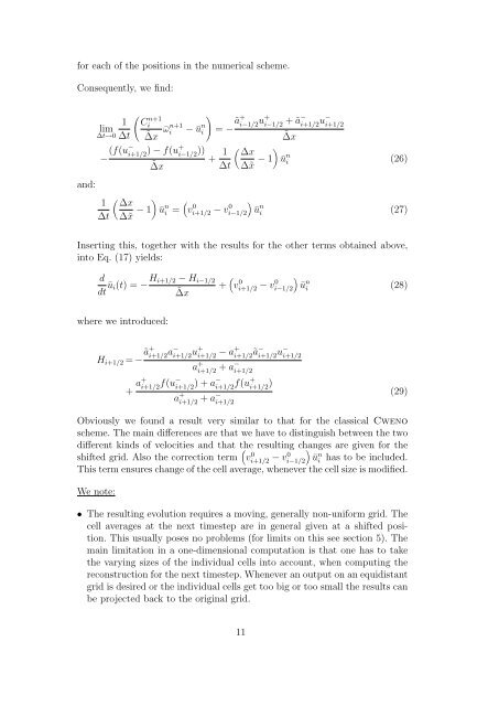
for each of the positions in the numerical scheme.
Consequently, we find:
and:
lim
∆t→0
( )
1 C
n+1
−ã+
i
∆t ˜∆x ¯ωn+1 i − ū n i−1/2
i = u+ i−1/2 + ã− i+1/2 u− i+1/2
˜∆x
− (f(u− i+1/2 ) − f(u+ i−1/2 ))
˜∆x
+ 1 ∆t
( ∆x
∆˜x − 1 )
ū n i (26)
( )
1 ∆x
∆t ∆˜x − 1 ū n i = ( vi+1/2 0 − vi−1/2) 0 ūn i (27)
Inserting this, together with the results for the other terms obtained above,
into Eq. (17) yields:
d
dtūi(t) = − H i+1/2 − H i−1/2
+ ( vi+1/2 ˜∆x
0 − vi−1/2) 0 ūn i (28)
where we introduced:
H i+1/2 = −ã+ i+1/2 a− i+1/2 u+ i+1/2 − a+ i+1/2ã− i+1/2 u− i+1/2
a + i+1/2 + a− i+1/2
+ a+ i+1/2 f(u− i+1/2 ) + a− i+1/2 f(u+ i+1/2 )
a + i+1/2 + a− i+1/2
(29)
Obviously we found a result very similar to that for the classical Cweno
scheme. The main differences are that we have to distinguish between the two
different kinds of velocities and that the resulting changes are given for the
shifted grid. Also the correction term ( v 0 i+1/2 − v0 i−1/2)
ūn i has to be included.
This term ensures change of the cell average, whenever the cell size is modified.
We note:
• The resulting evolution requires a moving, generally non-uniform grid. The
cell averages at the next timestep are in general given at a shifted position.
This usually poses no problems (for limits on this see section 5). The
main limitation in a one-dimensional computation is that one has to take
the varying sizes of the individual cells into account, when computing the
reconstruction for the next timestep. Whenever an output on an equidistant
grid is desired or the individual cells get too big or too small the results can
be projected back to the original grid.
11