Causal Inference: The R package pcalg
Causal Inference: The R package pcalg
Causal Inference: The R package pcalg

You also want an ePaper? Increase the reach of your titles
YUMPU automatically turns print PDFs into web optimized ePapers that Google loves.
JSS<br />
Journal of Statistical Software<br />
MMMMMM YYYY, Volume VV, Issue II.<br />
http://www.jstatsoft.org/<br />
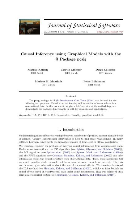
<strong>Causal</strong> <strong>Inference</strong> using Graphical Models with the<br />
R Package <strong>pcalg</strong><br />
Markus Kalisch<br />
ETH Zurich<br />
Martin Mächler<br />
ETH Zurich<br />
Diego Colombo<br />
ETH Zurich<br />
Marloes H. Maathuis<br />
ETH Zurich<br />
Peter Bühlmann<br />
ETH Zurich<br />
Abstract<br />
<strong>The</strong> <strong>pcalg</strong> <strong>package</strong> for R (R Development Core Team (2010)) can be used for the<br />
following two purposes: <strong>Causal</strong> structure learning and estimation of causal effects from<br />
observational data. In this document, we give a brief overview of the methodology, and<br />
demonstrate the <strong>package</strong>’s functionality in both toy examples and applications.<br />
Keywords: IDA, PC, RFCI, FCI, do-calculus, causality, graphical model, R.<br />
1. Introduction<br />
Understandingcause-effectrelationshipsbetweenvariablesisofprimaryinterestinmanyfields<br />
of science. Usually, experimental intervention is used to find these relationships. In many<br />
settings, however, experiments are infeasible because of time, cost or ethical constraints.<br />
We therefore consider the problem of inferring causal information from observational data.<br />
Under some assumptions, the PC algorithm (see Spirtes, Glymour, and Scheines (2000)),<br />
the FCI algorithm (see Spirtes et al. (2000) and Spirtes, Meek, and Richardson (1999a))<br />
and the RFCI algorithm (see Colombo, Maathuis, Kalisch, and Richardson (2012)) can infer<br />
information about the causal structure from observational data. Thus, these algorithms tell<br />
us which variables could or could not be a cause of some variable of interest. <strong>The</strong>y do<br />
not, however, give information about the size of the causal effects. We therefore developed<br />
the IDA method (see Maathuis, Kalisch, and Bühlmann (2009)), which can infer bounds on<br />
causal effects based on observational data under some assumptions. IDA was validated on a<br />
large-scale biological system (see Maathuis, Colombo, Kalisch, and Bühlmann (2010)).
2 <strong>Causal</strong> Graphical Models: Package <strong>pcalg</strong><br />
For broader use of these methods, well documented and easy to use software is indispensable.<br />
WethereforewrotetheR-<strong>package</strong><strong>pcalg</strong>, whichcontainsimplementationsofthePC-, FCI-and<br />
RFCI-algorithms, as well as of the IDA method. <strong>The</strong> objective of this paper is to introduce<br />
the R <strong>package</strong> <strong>pcalg</strong>, explain the range of functions on simulated data sets and summarize<br />
some applications.<br />
To get started, we show how two of the main functions (one for causal structure learning and<br />
one for estimating causal effects from observational data) can be used in a typical application.<br />
Suppose we have a system described by some variables and many observations of this<br />
system. Furthermore, assume that it seems plausible that there are no hidden variables and<br />
no feedback loops in the underlying causal system. <strong>The</strong> causal structure of such a system can<br />
be conveniently represented by a directed acyclic graph (DAG), where each node represents<br />
a variable and each directed edge represents a direct cause. To fix ideas, we have simulated<br />
an example data set with p = 8 continuous variables with Gaussian noise and n = 5000<br />
observations, which we will now analyse. First, we load the <strong>package</strong> <strong>pcalg</strong> and the data set.<br />
R> library("<strong>pcalg</strong>")<br />
R> data("gmG")<br />
In the next step, we use the function pc() to produce an estimate of the underlying causal<br />
structure. Sincethisfunctionisbasedonconditionalindependencetests, weneedtodefinetwo<br />
things. First, we need a function that can compute conditional independence tests in a way<br />
that is suitable for the data at hand. For standard data types (Gaussian, discrete and binary)<br />
we provide predefined functions. See the example section in the help file of pc() for more<br />
details. Secondly, weneedasummaryofthedata(sufficientstatistic)onwhichtheconditional<br />
independence function can work. Each conditional independence test can be performed at a<br />
certain significance level alpha. This can be treated as a tuning parameter. In the following<br />
code, we use the predefined function gaussCItest() as conditional independence test and<br />
create the corresponding sufficient statistic, consisting of the correlation matrix of the data<br />
and the sample size. <strong>The</strong>n we use the function pc() to estimate the causal structure and plot<br />
the result.<br />
R> suffStat pc.fit stopifnot(require(Rgraphviz))# needed for all our graph plots<br />
R> par(mfrow = c(1,2))<br />
R> plot(gmG$g, main = "")<br />
R> plot(pc.fit, main = "")<br />
As can be seen in Fig. 1, there are directed and bidirected edges in the estimated causal<br />
structure. <strong>The</strong> directed edges show the presence and direction of direct causal effects. A bidirected<br />
edge means that the PC-algorithm was unable to decide whether the edge orientation<br />
should be ← or →. Thus, bidirected edges represent some uncertainty in the resulting model.<br />
<strong>The</strong>y reflect the fact that in general one cannot estimate a unique DAG from observational<br />
data, not even with an infinite amount of data, since several DAGs can describe the same<br />
conditional independence information.<br />
On the inferred causal structure, we can estimate the causal effect of an intervention. Denote<br />
the variable corresponding to node i in the graph by V i . For example, suppose that, by<br />
external intervention, we first set the variable V 1 to some value ˜x, and then to the value ˜x+1.
Journal of Statistical Software 3<br />
1<br />
4<br />
1<br />
4<br />
2<br />
2<br />
3<br />
5<br />
3<br />
5<br />
6<br />
8<br />
6<br />
8<br />
7<br />
7<br />
Figure1: TrueunderlyingcausalDAG(left)andestimatedcausalstructure(right), representing<br />
a Markov equivalence class of DAGs that all encode the same conditional independence<br />
information. (Due to the large sample size, there were no sampling errors.)<br />
<strong>The</strong> recorded average change in variable V 6 is the (total) causal effect of V 1 on V 6 . More<br />
precisely, the causal effect C(V 1 ,V 6 ,˜x) of V 1 from V 1 = ˜x on V 6 is defined as<br />
C(V 1 ,V 6 ,˜x) = E(V 1 |do(V 6 = ˜x+1))−E(V 1 |do(V 6 = ˜x)) or<br />
C(V 1 ,V 6 ,˜x) = ∂<br />
∂x E(V 1|do(V 6 = x))| x=˜x ,<br />
where do(V 6 = x) denotes Pearl’s do-operator (see Pearl (2000)). If the causal relationships<br />
are linear, these two expressions are equivalent and do not depend on ˜x.<br />
Since the causal structure was not identified uniquely in our example, we cannot expect to<br />
get a unique number for the causal effect. Instead, we get a set of possible causal effects. This<br />
set can be computed by using the function ida(). To provide full quantitative information,<br />
we need to pass the covariance matrix in addition to the estimated causal structure.<br />
R> ida(1, 6, cov(gmG$x), pc.fit@graph)<br />
[1] 0.75364 0.54878<br />
Since we simulated the data, we know that the true value of the causal effect is 0.71. Thus,<br />
one of the two estimates is indeed close to the true value. Since both values are larger than<br />
zero, we can conclude that variable V 1 has a positive causal effect on variable V 6 . Thus, we<br />
can always estimate a lower bound for the absolute value of the causal effect. (Note that at<br />
this point we have no p-value to control the sampling error.)<br />
If we would like to know the effect of a unit increase in variable V 1 on variables V 4 , V 5 and<br />
V 6 , we could simply call ida() three times. However, a faster way is to call the function<br />
idaFast(), which was tailored for such situations.<br />
R> idaFast(1, c(4,5,6), cov(gmG$x), pc.fit@graph)
4 <strong>Causal</strong> Graphical Models: Package <strong>pcalg</strong><br />
[,1] [,2]<br />
4 0.01027 0.012014<br />
5 0.23875 0.017935<br />
6 0.75364 0.548776<br />
Each row in the output shows the estimated set of possible causal effects on the target variable<br />
indicated by the row names. <strong>The</strong> true values for the causal effects are 0, 0.2, 0.71 for variables<br />
V 4 , V 5 and V 6 , respectively. <strong>The</strong> first row, corresponding to variable V 4 , quite accurately<br />
indicates a causal effect that is very close to zero or no effect at all. <strong>The</strong> second row of the<br />
output, corresponding to variable V 5 , is rather uninformative: Although one entry comes close<br />
to the true value, the other estimate is close to zero. Thus, we cannot be sure if there is a<br />
causal effect at all. <strong>The</strong> third row, corresponding to V 6 was already discussed above.<br />
2. Methodological background<br />
InSection2.1weproposemethodsforestimatingthecausalstructurefromobservationaldata.<br />
In particular, we discuss the PC algorithm (see Spirtes et al. (2000))), the FCI algorithm (see<br />
Spirtes et al. (2000) and Spirtes et al. (1999a)) and the RFCI algorithm (see Colombo et al.<br />
(2012)). In Section 2.2 we describe the IDA method (see Maathuis et al. (2009)) to obtain<br />
bounds on causal effects from observational data. This method is based on first estimating<br />
the causal structure and then applying do-calculus (see Pearl (2000))<br />
2.1. Estimating causal structures with graphical models<br />
Graphical models can be thought of as maps of dependence structures of a given probability<br />
distribution or a sample thereof (see for example Lauritzen (1996)). In order to illustrate<br />
the analogy, let us consider a road map. In order to be able to use a road map, one needs<br />
two given factors. First, one needs the physical map with symbols such as dots and lines.<br />
Second, one needs a rule for interpreting the symbols. For instance, a railroad map and a<br />
map for electric circuits might look very much alike, but their interpretation differs a lot. In<br />
the same sense, a graphical model is a map. First, a graphical model consists of a graph with<br />
dots, lines and potentially edge marks like arrowheads or circles. Second, a graphical model<br />
always comes with a rule for interpreting this graph. In general, nodes in the graph represent<br />
(random) variables and edges represent some kind of dependence.<br />
Without hidden and selection variables<br />
An example of a graphical model is the DAG model. <strong>The</strong> physical map here is a graph<br />
consisting of nodes and directed edges (← or →). As a further restriction, the edges must be<br />
directed in a way, so that it is not possible to trace a cycle when following the arrowheads<br />
(i.e., no directed cycles). <strong>The</strong> interpretation rule is called d-separation. This rule is a bit<br />
intricate and we refer the reader to Lauritzen (1996) for more details. This interpretation<br />
rule can be used in the following way: If two nodes x and y are d-separated by a set of nodes<br />
S, then the corresponding random variables V x and V y are conditionally independent given<br />
the set of random variables V S . For the following, we only deal with distributions where the<br />
following holds: For each distribution, it is possible to find a DAG, whose list of d-separation<br />
relations perfectly matches the list of conditional independencies of the distribution. Such<br />
distributions are called faithful. It has been shown that the set of distributions that are
Journal of Statistical Software 5<br />
faithful is the overwhelming majority (Meek (1995)), so that the assumption does not seem<br />
to be very strict in practice.<br />
Since the DAG model encodes conditional independencies, it seems plausible that information<br />
on the latter helps to infer aspects of the former. This intuition is made precise in the PC<br />
algorithm (see Spirtes et al. (2000); PC stands for the initials of its inventors Peter Spirtes<br />
and Clark Glymour) which was proven to reconstruct the structure of the underlying DAG<br />
model given a conditional independence oracle up to its Markov equivalence class which is<br />
discussed in more detail below. In practice, the conditional independence oracle is replaced<br />
by a statistical test for conditional independence. For situations without hidden variables<br />
and under some further conditions it has been shown that the PC algorithm using statistical<br />
tests instead of an independence oracle is computationally feasible and consistent even for<br />
very high-dimensional sparse DAGs (see Kalisch and Bühlmann (2007)).<br />
As mentioned before, several DAGs can encode the same list of conditional independencies.<br />
One can show that such DAGs must share certain properties. To be more precise, we have to<br />
define a v-structure as the subgraph i → j ← k on the nodes i, j and k where i and k are not<br />
adjacent (i.e., , there is no edge between i and k). Furthermore, let the skeleton of a DAG be<br />
the graph that is obtained by removing all arrowheads from the DAG. It was shown that two<br />
DAGs encode the same conditional independence statements if and only if the corresponding<br />
DAGs have the same skeleton and the same v-structures (see Verma and Pearl (1991)). Such<br />
DAGs are called Markov-equivalent. In this way, the space of DAGs can be partitioned into<br />
equivalence classes, where all members of an equivalence class encode the same conditional<br />
independence information. Conversely, if given a conditional independence oracle, one can<br />
only determine a DAG up to its equivalence class. <strong>The</strong>refore, the PC algorithm cannot<br />
determine the DAG uniquely, but only the corresponding equivalence class of the DAG.<br />
An equivalence class can be visualized by a graph that has the same skeleton as every DAG in<br />
the equivalence class and directed edges only where all DAGs in the equivalence class have the<br />
same directed edge. Edges that point into one direction for some DAGs in the equivalence<br />
class and in the other direction for other DAGs in the equivalence class are visualized by<br />
bidirected edges (sometimes, undirected edges are used instead). This graph is called a<br />
completed partially directed acyclic graph (CPDAG).<br />
Algorithm 1 Outline of the PC-algorithm<br />
Input: Vertex set V, conditional independence information, significance level α<br />
Output: Estimated CPDAG Ĝ, separation sets Ŝ<br />
Edge types: →, −<br />
(P1) Form the complete undirected graph on the vertex set V<br />
(P2) Test conditional independence given subsets of adjacency sets at a given significance<br />
level α and delete edges if conditional independent<br />
(P3) Orient v-structures<br />
(P4) Orient remaining edges.<br />
We now describe the PC-algorithm, which is shown in Algorithm 1, in more detail. <strong>The</strong><br />
PC-algorithm starts with a complete undirected graph, G 0 , as stated in (P1) of Algorithm 1.<br />
In stage (P2), a series of conditional independence tests is done and edges are deleted in the<br />
following way. First, all pairs of nodes are tested for marginal independence. If two nodes i<br />
and j are judged to be marginally independent at level α, the edge between them is deleted
6 <strong>Causal</strong> Graphical Models: Package <strong>pcalg</strong><br />
and the empty set is saved as separation sets Ŝ[i,j] and Ŝ[j,i]. After all pairs have been<br />
tested for marginal independence and some edges might have been removed, a graph results<br />
which we denote by G 1 . In the second step, all pairs of nodes (i,j) still adjacent in G 1 are<br />
tested for conditional independence given any single node in adj(G 1 ,i)\{j} or adj(G 1 ,j)\{i}<br />
(adj(G,i) denotes the set of nodes in graph G that are adjacent to node i) . If there is any<br />
node k such that V i and V j are conditionally independent given V k , the edge between i and<br />
j is removed and node k is saved as separation sets (sepset) Ŝ[i,j] and Ŝ[j,i]. If all adjacent<br />
pairs have been tested given one adjacent node, a new graph results which we denote by G 2 .<br />
<strong>The</strong> algorithm continues in this way by increasing the size of the conditioning set step by step.<br />
<strong>The</strong> algorithm stops if all adjacency sets in the current graph are smaller than the size of the<br />
conditioning set. <strong>The</strong> result is the skeleton in which every edge is still undirected. Within<br />
(P3), each triple of vertices (i,k,j) such that the pairs (i,k) and (j,k) are each adjacent<br />
in the skeleton but (i,j) are not (such a triple is called an “unshielded triple”), is oriented<br />
based on the information saved in the conditioning sets Ŝ[i,j] and Ŝ[j,i]. More precisely, an<br />
unshielded triple i−k −j is oriented as i → k ← j if k is not in Ŝ[j,i] = Ŝ[i,j]. Finally, in<br />
(P4) it may be possible to orient some of the remaining edges, since one can deduce that one<br />
of the two possible directions of the edge is invalid because it introduces a new v-structure<br />
or a directed cycle. Such edges are found by repeatedly applying rules described in Spirtes<br />
et al. (2000), p.85. <strong>The</strong> resulting output is the equivalence class (CPDAG) that describes the<br />
conditional independence information in the data, in which every edge is either undirected or<br />
directed. (To simplify visual presentation, undirected edges are depicted as bidirected edges<br />
in the output as soon as at least one directed edge is present. If no directed edge is present,<br />
all edges are undirected.)<br />
A causal structure without feedback loops and without hidden or selection variable can be<br />
visualized using a DAG where the edges indicate direct cause-effect relationships. Under some<br />
assumptions, Pearl (2000) showed (Th. 1.4.1) that there is a link between causal structures<br />
and graphical models. Roughly speaking, if the underlying causal structure is a DAG, we<br />
observe data generated from this DAG and then estimate a DAG model (i.e., a graphical<br />
model) on this data, the estimated CPDAG represents the equivalence class of the DAG<br />
model describing the causal structure. This holds if we have enough samples and assuming<br />
thatthetrueunderlyingcausalstructureisindeedaDAGwithoutlatentorselectionvariables.<br />
Note that even given an infinite amount of data, we usually cannot identify the true DAG<br />
itself, but only its equivalence class. Every DAG in this equivalence class can be the true<br />
causal structure.<br />
With hidden or selection variables<br />
When discovering causal relations from nonexperimental data, two difficulties arise. One<br />
is the problem of hidden (or latent) variables: Factors influencing two or more measured<br />
variables may not themselves be measured. <strong>The</strong> other is the problem of selection bias: Values<br />
of unmeasured variables or features may influence whether a unit is included in the data<br />
sample.<br />
In the case of hidden or selection variables, one could still visualize the underlying causal<br />
structure with a DAG that includes all observed, hidden and selection variables. However,<br />
when inferring the DAG from observational data, we do not know all hidden and selection<br />
variables.
Journal of Statistical Software 7<br />
Wethereforeseektofindastructurethatrepresentsallconditionalindependencerelationships<br />
among the observed variables given the selection variables of the underlying causal structure.<br />
It turns out that this is possible. However, the resulting object is in general not a DAG<br />
for the following reason. Suppose, we have a DAG including observed, latent and selection<br />
variables and we would like to visualize the conditional independencies among the observed<br />
variables only. We could marginalize out all latent variables and condition on all selection<br />
variables. It turns out that the resulting list of conditional independencies can in general not<br />
be represented by a DAG, since DAGs are not closed under marginalization or conditioning<br />
(see Richardson and Spirtes (2002)).<br />
A class of graphical independence models that is closed under marginalization and conditioning<br />
and that contains all DAG models is the class of ancestral graphs. A detailed discussion<br />
of this class of graphs can be found in Richardson and Spirtes (2002). In this text, we only<br />
give a brief introduction.<br />
Ancestral graphs have nodes, which represent random variables and edges which represent<br />
some kind of dependence. <strong>The</strong> edges can be either directed (← or →), undirected (-) or<br />
bidirected (↔) (note that in the context of ancestral graphs, undirected and bidirected edges<br />
do not mean the same). <strong>The</strong>re are two rules that restrict the direction of edges in an ancestral<br />
graph:<br />
1: If i and j are joined by an edge with an arrowhead at i, then there is no directed path<br />
from i to j. (A path is a sequence of adjacent vertices, and a directed path is a path<br />
along directed edges that follows the direction of the arrowheads.)<br />
2: <strong>The</strong>re are no arrowheads present at a vertex which is an endpoint of an undirected edge.<br />
Maximal ancestral graphs (MAG), which we will use from now on, also obey a third rule:<br />
3: Every missing edge corresponds to a conditional independence.<br />
<strong>The</strong> conditional independence statements of MAGs can be read off using the concept of m-<br />
separation, which is a generalization the concept of d-separation. Furthermore, part of the<br />
causal information in the underlying DAG is represented in the MAG. If in the MAG there<br />
is an edge between node i and node j with an arrowhead at node i, then there is no directed<br />
path from node i to node j nor to any of the selection variables in the underlying DAG (i.e.,<br />
, i is not a cause of j or of the selection variables). If, on the other hand, there is a tail at<br />
node i, then there is a directed path from node i to node j or to one of the selection variables<br />
in the underlying DAG (i.e., , i is a cause of j or of a selection variable).<br />
Recall that finding a unique DAG from an independence oracle is in general impossible.<br />
<strong>The</strong>refore, one only reports on the equivalence class of DAGs in which the true DAG must<br />
lie. <strong>The</strong> equivalence class is visualized using a CPDAG. <strong>The</strong> same is true for MAGs: Finding<br />
a unique MAG from an independence oracle is in general impossible. One only reports on the<br />
equivalence class in which the true MAG lies.<br />
An equivalence class of a MAG can be uniquely represented by a partial ancestral graph<br />
(PAG) (see e.g., Zhang (2008)). A PAG contains the following types of edges: o–o, o–, o–>,<br />
–>, , –. Roughly, the bidirected edges come from hidden variables, and the undirected<br />
edges come from selection variables. <strong>The</strong> edges have the following interpretation: (i) <strong>The</strong>re<br />
is an edge between x and y if and only if V x and V y are conditionally dependent given V S for
8 <strong>Causal</strong> Graphical Models: Package <strong>pcalg</strong><br />
all sets V S consisting of all selection variables and a subset of the observed variables; (ii) a<br />
tail on an edge means that this tail is present in all MAGs in the equivalence class; (iii) an<br />
arrowhead on an edge means that this arrowhead is present in all MAGs in the equivalence<br />
class; (iv) a o-edgemark means that there is a at least one MAG in the equivalence class where<br />
the edgemark is a tail, and at least one where the edgemark is an arrowhead.<br />
An algorithm for finding the PAG given an independence oracle is the FCI algorithm (“fast<br />
causal inference”; see Spirtes et al. (2000) and Spirtes, Meek, and Richardson (1999b)). <strong>The</strong><br />
orientation rules of this algorithm were slightly extended and proven to be complete in Zhang<br />
(2008). FCI is very similar to PC but makes additional conditional independence tests and<br />
uses more orientation rules (see Section 3.3 for more details). We refer the reader to Zhang<br />
(2008) or Colombo et al. (2012) for a detailed discussion of the FCI algorithm. It turns out<br />
that the FCI algorithm is computationally infeasible for large graphs. <strong>The</strong> RFCI algorithm<br />
(“really fast causal inference”; see Colombo et al. (2012)), is much faster than FCI. <strong>The</strong><br />
output of RFCI is in general slightly less informative than the output of FCI, in particular<br />
with respect to conditional independence information. However, it was shown in Colombo<br />
et al. (2012) that any causal information in the output of RFCI is correct and that both FCI<br />
andRFCIareconsistentin(different)sparsehigh-dimensionalsettings. Finally, insimulations<br />
the estimation performances of the algorithms are very similar.<br />
2.2. Estimating bounds on causal effects<br />
One way of quantifying the causal effect of variable V x on V y is to measure the state of V y if<br />
V x is forced to take value V x = x and compare this to the value of V y if V x is forced to take<br />
the value V x = x+1 or V x = x+δ. If V x and V y are random variables, forcing V x = x could<br />
have the effect of changing the distribution of V y . Following the conventions in Pearl (2000),<br />
the resulting distribution after manipulation is denoted by P[V y |do(V x = x)]. Note that this<br />
is different from the conditional distribution P[V y |V x = x]. To illustrate this, imagine the<br />
following simplistic situation. Suppose we observe a particular spot on the street during some<br />
hour. <strong>The</strong> random variable V x denotes whether it rained during that hour (V x = 1 if it rained,<br />
V x = 0 otherwise). <strong>The</strong> random variable V y denotes whether the street was wet at the end of<br />
that hour (V y = 1 if it was wet, V y = 0 otherwise). If we assume P(V x = 1) = 0.1 (rather dry<br />
region), P(V y = 1|V x = 1) = 0.99 (the street is almost always still wet at the end of the hour<br />
when it rained during that hour) and P(V y = 1|V x = 0) = 0.02 (other reasons for making the<br />
street wet are rare), we can compute the conditional probability P(V x = 1|V y = 1) = 0.85.<br />
So, if we observe the street to be wet, the probability that there was rain in the last hour is<br />
about 0.85. However, if we take a garden hose and force the street to be wet at a randomly<br />
chosen hour, we get P(V x = 1|do(V y = 1)) = P(V x = 1) = 0.1. Thus, the distribution of the<br />
random variable describing rain is quite different when making an observation versus making<br />
an intervention.<br />
Oftentimes, only the change of the target distribution under intervention is reported. We use<br />
∂<br />
the change in mean, i.e.,<br />
∂x E[V y|do(V x = x)], as a general measure for the causal effect of<br />
V x on V y . For multivariate Gaussian random variables, E[V y |do(V x = x)] depends linearly<br />
on x. <strong>The</strong>refore, the derivative is constant which means that the causal effect does not<br />
depend on x, and can also be interpreted as E[V y |do(V x = x + 1)] − E[V y |do(V x = x)]. For<br />
binary random variables (with domain {0,1}) we define the causal effect of V x on V y as<br />
E(V y |do(V x = 1))−E(V y |do(V x = 0)) = P(V y = 1|do(V x = 1))−P(V y = 1|do(V x = 0)).
Journal of Statistical Software 9<br />
<strong>The</strong> goal in the remainder of this section is to estimate the effect of an intervention if only<br />
observational data is available.<br />
Without hidden and selection variables<br />
If the causal structure is a known DAG and there are no hidden and selection variables, Pearl<br />
(2000) (Th 3.4.1) suggested a set of inference rules known as “do-calculus” whose application<br />
transforms an expression involving a“do”into an expression involving only conditional<br />
distributions. Thus, information on the interventional distribution can be obtained by using<br />
information obtained by observations and knowledge of the underlying causal structure.<br />
Unfortunately, the causal structure is rarely known in practice. However, as discussed in<br />
Section 2.1, we can estimate the Markov equivalence class of the true causal DAG. Taking<br />
this into account, we conceptually apply the do-calculus on each DAG within the equivalence<br />
classandthusobtainapossiblecausaleffectforeachDAGintheequivalenceclass(inpractice,<br />
we developed a local method that is faster but yields a similar result; see Section 3.5 for more<br />
details). <strong>The</strong>refore, even if we have an infinite amount of observations we can in general report<br />
on a multiset of possible causal values (it is a multiset rather than a set because it can contain<br />
duplicatevalues). Oneofthesevaluesisthetruecausaleffect. Despitetheinherentambiguity,<br />
this result can still be very useful when the multiset has certain properties (e.g., all values<br />
are much larger than zero). <strong>The</strong>se ideas are incorporated in the IDA method (Intervention<br />
calculus when the DAG is Absent).<br />
In addition to this fundamental limitation in estimating a causal effect, errors due to finite<br />
sample size blur the result as with every statistical method. Thus, we can typically only get<br />
an estimate of the set of possible causal values. It was shown that this estimate is consistent<br />
in sparse high-dimensional settings under some assumptions by Maathuis et al. (2009).<br />
It has recently been shown empirically that despite the described fundamental limitations<br />
in identifying the causal effect uniquely and despite potential violations of the underlying<br />
assumptions, the method performs well in identifying the most important causal effects in a<br />
high-dimensional yeast gene expression data set (see Maathuis et al. (2010)).<br />
With hidden and selection variables<br />
At the moment, we can not yet estimate causal effects when hidden variables or selection<br />
variables are present.<br />
2.3. Summary of assumptions<br />
For all proposed methods, we assume that the data is faithful to the unknown underlying<br />
causal DAG. For the individual methods, further assumptions are made.<br />
PC-algorithm: No hidden or selection variables; consistent in high-dimensional settings<br />
(the number of variables grows with the sample size) if the underlying DAG is sparse,<br />
the data is multivariate Normal and satisfies some regularity conditions on the partial<br />
correlations, and α is taken to zero appropriately. See Kalisch and Bühlmann (2007)<br />
for full details. Consistency in a standard asymptotic regime with a fixed number of<br />
variables follows as a special case.<br />
FCI-algorithm: Allows for hidden and selection variables; consistent in high-dimensional
10 <strong>Causal</strong> Graphical Models: Package <strong>pcalg</strong><br />
settings if the so-called Possible-D-SEP sets (see Spirtes et al. (2000)) are sparse, the<br />
data is multivariate Normal and satisfies some regularity conditions on the partial correlations,<br />
and α is taken to zero appropriately. See Colombo et al. (2012) for full details.<br />
Consistency in a standard asymptotic regime with a fixed number of variables follows<br />
as a special case.<br />
RFCI-algorithm: Allows for hidden and selection variables; consistent in high-dimensional<br />
settings if the underlying MAG is sparse (this is a much weaker assumption than the one<br />
needed for FCI), the data is multivariate Normal and satisfies some regularity conditions<br />
on the partial correlations, and α is taken to zero appropriately. See Colombo et al.<br />
(2012) for full details. Consistency in a standard asymptotic regime with a fixed number<br />
of variables follows as a special case.<br />
IDA: No hidden or selection variables; all conditional expectations are linear; consistent in<br />
high-dimensional settings if the underlying DAG is sparse, the data is multivariate Normal<br />
and satisfies some regularity conditions on the partial correlations and conditional<br />
variances, and α is taken to zero appropriately. See Maathuis et al. (2009) for full<br />
details.<br />
3. Package <strong>pcalg</strong><br />
This<strong>package</strong>hastwogoals. First, itisintendedtoprovidefast, flexibleandreliableimplementations<br />
of the PC, FCI and RFCI algorithms for estimating causal structures and graphical<br />
models. Second, it provides an implementation of the IDA method, which estimates bounds<br />
on causal effects from observational data when no causal structure is known and hidden or<br />
selection variables are absent.<br />
In the following, we describe the main functions of our <strong>package</strong> for achieving these goals.<br />
<strong>The</strong> functions skeleton(), pc(), fci() and rfci() are intended for estimating graphical<br />
models. <strong>The</strong> functions ida() and idaFast() are intended for estimating causal effects from<br />
observational data.<br />
Alternatives to this <strong>package</strong> for estimating graphical models in R include: Scutari (2010),<br />
Bottcher and Dethlefsen (2011), Hojsgaard (2012), Hojsgaard, Dethlefsen, and Bowsher<br />
(2012) and Hojsgaard and Lauritzen (2011).<br />
3.1. skeleton<br />
<strong>The</strong> function skeleton() implements (P1) and (P2) from Algorithm 1. <strong>The</strong> function can be<br />
called with the following arguments<br />
skeleton(suffStat, indepTest, p, alpha, verbose = FALSE, fixedGaps = NULL,<br />
fixedEdges = NULL, NAdelete = TRUE, m.max = Inf)<br />
As was discussed in Section 2.1, the main task in finding the skeleton is to compute and<br />
test several conditional independencies. To keep the function flexible, skeleton() takes as<br />
argument a function indepTest() that performs these conditional independence tests and<br />
returns a p-value. All information that is needed in the conditional independence test can<br />
be passed in the argument suffStat. <strong>The</strong> only exceptions are the number of variables p
Journal of Statistical Software 11<br />
R> require("<strong>pcalg</strong>")<br />
R> data("gmG")<br />
R> suffStat pc.fit par(mfrow = c(1,2))<br />
R> plot(gmG$g, main = "")<br />
R> plot(pc.fit, main = "")<br />
1<br />
4<br />
1<br />
4<br />
2<br />
2<br />
3<br />
5<br />
3<br />
5<br />
6<br />
8<br />
6<br />
8<br />
7<br />
7<br />
Figure 2: True underlying DAG (left) and estimated skeleton (right) fitted on the simulated<br />
Gaussian data set gmG.<br />
and the significance level alpha for the conditional independence tests, which are passed<br />
separately. For convenience, we have preprogrammed versions of indepTest() for Gaussian<br />
data (gaussCItest()), discrete data (disCItest()), and binary data (binCItest()). Each<br />
of these independence test functions needs different arguments as input, described in the<br />
respective help files. For example, when using gaussCItest(), the input has to be a list<br />
containing the correlation matrix and the sample size of the data. In the following code, we<br />
estimate the skeleton on the data set gmG (which consists of p = 8 variables and n = 5000<br />
samples)andplotthe results. <strong>The</strong> estimated skeletonandthe trueunderlying DAGare shown<br />
in Fig. 2.<br />
To give another example, we show how to fit a skeleton to the example data set gmD (which<br />
consists of p = 5 discrete variables with 3, 2, 3, 4 and 2 levels and n = 10000 samples). <strong>The</strong><br />
predefined test function disCItest() is based on the G 2 statistic and takes as input a list<br />
containing the data matrix, a vector specifying the number of levels for each variable and an<br />
option which indicates if the degrees of freedom must be lowered by one for each zero count.<br />
Finally, we plot the result. <strong>The</strong> estimated skeleton and the true underlying DAG are shown<br />
in Fig. 3.<br />
In some situations, one may have prior information about the underlying DAG, for example<br />
that certain edges are absent or present. Such information can be incorporated into the<br />
algorithm via the arguments fixedGaps (absent edges) and fixedEdges (present edges). <strong>The</strong>
12 <strong>Causal</strong> Graphical Models: Package <strong>pcalg</strong><br />
1 2<br />
3 4<br />
5<br />
1 2<br />
3 4<br />
5<br />
Figure 3: True underlying DAG (left) and estimated skeleton (right) fitted on the simulated<br />
discrete data set gmD.<br />
information in fixedGaps and fixedEdges is used as follows. <strong>The</strong> gaps given in fixedGaps<br />
are introduced in the very beginning of the algorithm by removing the corresponding edges<br />
from the complete undirected graph. Thus, these edges are guaranteed to be absent in the<br />
resulting graph. Pairs (i,j) in fixedEdges are skipped in all steps of the algorithm, so that<br />
these edges are guaranteed to be present in the resulting graph.<br />
IfindepTest()returnsNAandtheoptionNAdeleteisTRUE,thecorrespondingedgeisdeleted.<br />
If this option is FALSE, the edge is not deleted.<br />
<strong>The</strong> argument m.max is the maximum size of the conditioning sets that are considered in the<br />
conditional independence tests in (P2) of Algorithm 1.<br />
Throughout, the function works with the column positions of the variables in the adjacency<br />
matrix, and not with the names of the variables.<br />
3.2. pc<br />
<strong>The</strong> function pc() implements all steps (P1) to (P4) of the PC algorithm shown in display<br />
algorithm 1. First, the skeleton is computed using the function skeleton() (steps (P1) and<br />
(P2)). <strong>The</strong>n, as many edges as possible are oriented (steps (P3) and (P4)). <strong>The</strong> function can<br />
be called as<br />
pc(suffStat, indepTest, p, alpha, verbose = FALSE, fixedGaps = NULL,<br />
fixedEdges = NULL, NAdelete = TRUE, m.max = Inf, u2pd = "rand",<br />
conservative = FALSE)<br />
where the arguments suffStat, indepTest, p, alpha, fixedGaps, fixedEdges, NAdelete<br />
and m.max are identical to those of skeleton().<br />
Samplingerrors(orhiddenvariables)canleadtoconflictinginformationaboutedgedirections.<br />
For example, one may find that a−b−c and b−c−d should both be oriented as v-structures.<br />
This gives conflicting information about the edge b−c, since it should be oriented as b ← c<br />
in v-structure a → b ← c, while it should be oriented as b → c in v-structure b → c ← d. In
Journal of Statistical Software 13<br />
such cases, we simply overwrite the directions of the conflicting edge. In the example above<br />
this means that we obtain a → b → c ← d if a−b−c was visited first, and a → b ← c ← d if<br />
b−c−d was visited first.<br />
Sampling errors or hidden variables can also lead to invalid CPDAGs, meaning that there<br />
does not exist a DAG that has the same skeleton and v-structures as the graph found by the<br />
algorithm. An example of this is an undirected cycle consisting of the edges a−b−c−d and<br />
d − a. In this case it is impossible to direct the edges without creating a cycle or a new v-<br />
structure. <strong>The</strong> optional argument u2pd specifies what should be done in such a situation. If it<br />
issetto"relaxed",thealgorithmsimplyoutputstheinvalidCPDAG.Ifu2pdissetto"rand",<br />
all direction information is discarded and a random DAG is generated on the skeleton. <strong>The</strong><br />
corresponding CPDAG is then returned. If u2pd is set to "retry", up to 100 combinations of<br />
possible directions of the ambiguous edges are tried, and the first combination that results in<br />
a valid CPDAG is chosen. If no valid combination is found, an arbitrary CPDAG is generated<br />
on the skeleton as with u2pd = "rand".<br />
By setting the argument conservative = TRUE, the conservative PC algorithm (see Ramsey,<br />
Zhang, and Spirtes (2006)) is chosen. <strong>The</strong> conservative PC is a slight variation of the PC<br />
algorithm and is intended to be more robust against sampling errors in its edge orientations.<br />
Aftertheskeletoniscomputed, allunshieldedtripletsa−b−carecheckedinthefollowingway.<br />
We test whether V a and V c are conditionally independent given any subset of the adjacency<br />
set of a or any subset of the adjacency set of c. If b is in no such conditioning set (and not<br />
in the original sepset) or in all such conditioning sets (and in the original sepset), the triple<br />
is marked as faithful. If, however, b is in some conditioning sets but not in others, or if there<br />
was no subset S of the adjacency set of a nor of c such that V a and V c are conditionally<br />
independent given V S , the triple is marked as“unfaithful”. Only faithful triples are oriented<br />
as v-structures. Furthermore, orientation rules that need to know whether a − b − c is a<br />
v-structure or not are only applied to faithful triples. (For more details, see the help file of<br />
the internal function pc.cons.intern() which is called with the argument version.unf =<br />
c(2,2).)<br />
As with the skeleton, the PC algorithm works with the column positions of the variables in<br />
the adjacency matrix, and not with the names of the variables. When plotting the object,<br />
undirected and bidirected edges are equivalent.<br />
As an example, we estimate a CPDAG of the Gaussian data used in the example for the<br />
skeleton in Section 3.1. Again, we choose the predefined gaussCItest() as conditional independence<br />
test and create the corresponding test statistic. Finally, we plot the result. <strong>The</strong><br />
estimated CPDAG and the true underlying DAG are shown in Fig. 4.<br />
3.3. fci<br />
<strong>The</strong> FCI algorithm is a generalization of the PC algorithm, in the sense that it allows arbitrarily<br />
many latent and selection variables. Under the assumption that the data are faithful<br />
to a DAG that includes all latent and selection variables, the FCI algorithm estimates the<br />
equivalence class of MAGs that describe the conditional independence relationships between<br />
the observed variables given the selection variables.<br />
<strong>The</strong> first part of the FCI algorithm is analogous to the PC algorithm. It starts with a<br />
complete undirected graph and estimates an initial skeleton using the function skeleton().<br />
All edges of this skeleton are of the form o–o. Now, the v-structures are oriented as in the
14 <strong>Causal</strong> Graphical Models: Package <strong>pcalg</strong><br />
R> suffStat pc.fit par(mfrow = c(1,2))<br />
R> plot(gmG$g, main = "")<br />
R> plot(pc.fit, main = "")<br />
1<br />
4<br />
1<br />
4<br />
2<br />
2<br />
3<br />
5<br />
3<br />
5<br />
6<br />
8<br />
6<br />
8<br />
7<br />
7<br />
Figure 4: True underlying DAG (left) and estimated CPDAG (right) fitted on the simulated<br />
Gaussian data set gmG.<br />
PC algorithm. However, due to the presence of hidden variables, it is no longer sufficient<br />
to consider only subsets of the adjacency sets of nodes x and y to decide whether the edge<br />
x−y should be removed. <strong>The</strong>refore, the initial skeleton may contain some superfluous edges.<br />
<strong>The</strong>se edges are removed in the next step of the algorithm. To decide whether edge x o–<br />
o y should be removed, one computes Possible-D-SEP(x, y) and Possible-D-SEP(y, x) and<br />
performs conditional independence tests of V x and V y given all subsets of Possible-D-SEP(x,<br />
y) and of Possible-D-SEP(y, x) (see helpfile of function pdsep()). Subsequently, all edges are<br />
transformed into o–o again and the v-structures are newly determined (using information in<br />
sepset). Finally, as many undetermined edge marks (o) as possible are determined using (a<br />
subset of) the 10 orientation rules given by Zhang (2008).<br />
<strong>The</strong> function can be called with the following arguments:<br />
fci(suffStat, indepTest, p, alpha, verbose = FALSE, fixedGaps = NULL,<br />
fixedEdges = NULL, NAdelete = TRUE, m.max = Inf, rules = rep(TRUE,<br />
10), doPdsep = TRUE, conservative = c(FALSE, FALSE),<br />
biCC = FALSE, cons.rules = FALSE, labels = NA)<br />
where the arguments suffStat, indepTest, p, alpha, fixedGaps, fixedEdges, NAdelete<br />
and m.max are identical to those in skeleton(). <strong>The</strong> option rules contains a logical vector<br />
of length 10 indicating which rules should be used when directing edges, where the order of<br />
the rules is taken from Zhang (2008).<br />
<strong>The</strong> option doPdsep indicates whether Possible-D-SEP should be computed for all nodes, and<br />
all subsets of Possible-D-SEP are considered as conditioning sets in the conditional independence<br />
tests. If FALSE, Possible-D-SEP is not computed, so that the algorithm simplifies to
Journal of Statistical Software 15<br />
the Modified PC algorithm of Spirtes et al. (2000).<br />
<strong>The</strong> argument conservative can be used to invoke the conservative FCI algorithm which<br />
consists of two parts. In the first part (done if conservative[1] is TRUE), we call the internal<br />
function pc.cons.internal() with argument version.unf = c(1,2) after computing the<br />
skeleton. This is a slight variation of the conservative PC algorithm (which usedversion.unf<br />
= c(2,2)): If V a is independent of V c given some V S in the skeleton (i.e., , the edge a − c<br />
droppedout), butV a andV c remaindependentgivenallsubsetsoftheadjacencysetofeithera<br />
or c, we call a−b−c“unambiguous”. This is because in the FCI algorithm, the true separating<br />
set might be outside the adjacency sets of a or c. <strong>The</strong> purpose of this conservative version is to<br />
speed up the algorithm in the sample version (less v-structures lead to smaller Possible-D-SEP<br />
sets). Inthesecondpart(doneifconservative[2]isTRUE),wecallpc.cons.internal(...,<br />
version.unf = c(1,2)) again after Possible-D-SEP was found and the graph potentially<br />
lost some edges. <strong>The</strong>refore, new triples might have occurred. If this second part is done, the<br />
resulting information on sepset and faithful triples overwrites the previous and will be used<br />
for the subsequent orientation rules. <strong>The</strong> purpose of this conservative version is used in the<br />
hope to obtain better edge orientations. See Colombo et al. (2012) for more details.<br />
By setting the argument biCC = TRUE, Possible-D-SEP(a, c) is defined as the intersection of<br />
the original Possible-D-SEP(a, c) and the set of nodes that lie on a path between a and c.<br />
This method uses biconnected components to find all nodes on a path between nodes a and c.<br />
<strong>The</strong> smaller Possible-D-SEP sets lead to faster computing times, while Colombo et al. (2012)<br />
showed that the algorithm is identical to the original FCI algorithm given oracle information<br />
on the conditional independence relationships.<br />
<strong>The</strong> argument cons.rules manages the way in which the information about unfaithful triples<br />
affects the orientation rules for directing edges. If cons.rules = TRUE, an orientation rule<br />
that needs information on definite non-colliders is only applied, if the corresponding subgraph<br />
relevant for the rule does not involve an unfaithful triple.<br />
Using the argument labels, one can pass names for the vertices of the estimated graph. By<br />
default, this argument is set to NA, in which case the node names as.character(1:p) are<br />
used.<br />
As an example, we estimate the PAG of a graph with five nodes using the function fci() and<br />
the predefined function gaussCItest() as conditional independence test. In Fig. 5 the true<br />
DAG and the PAG estimated with fci() are shown. Random variable V 1 is latent. We can<br />
read off that both V 4 and V 5 cannot be a cause of V 2 and V 3 , which can be confirmed in the<br />
true DAG.<br />
R> data("gmL")<br />
R> suffStat1 pag.est par(mfrow = c(1,2))<br />
R> plot(gmL$g, main = "")<br />
R> plot(pag.est)<br />
3.4. rfci<br />
<strong>The</strong> function rfci() is rather similar to fci(). However, it does not compute any Possible-
16 <strong>Causal</strong> Graphical Models: Package <strong>pcalg</strong><br />
1 2<br />
3 4<br />
5<br />
2 3<br />
●<br />
4<br />
●<br />
●<br />
●<br />
5<br />
●<br />
●<br />
Figure 5: True underlying DAG (left) and estimated PAG (right), when applying the FCI<br />
and RFCI algorithms to the data set gmL. <strong>The</strong> output of FCI and RFCI is identical. Variable<br />
V 1 of the true underlying DAG is latent.<br />
D-SEP sets and thus does not make tests conditioning on them. This makes rfci() much<br />
faster than fci(). <strong>The</strong> orientation rule for v-structures and the orientation rule for so-called<br />
discriminating paths (rule 4) were modified in order to produce a PAG which, in the oracle<br />
version, is guaranteed to have correct ancestral relationships.<br />
<strong>The</strong> function can be called in the following way:<br />
rfci(suffStat, indepTest, p, alpha, verbose = FALSE, fixedGaps = NULL,<br />
fixedEdges = NULL, NAdelete = TRUE, m.max = Inf)<br />
where the arguments suffStat, indepTest, p, alpha, fixedGaps, fixedEdges, NAdelete<br />
and m.max are identical to those in skeleton().<br />
As an example, we re-run the example from Section 3.3 and show the PAG estimated with<br />
rfci() in Figure 5. <strong>The</strong> PAG estimated with fci() and the PAG estimated with rfci() are<br />
the same.<br />
R> data("gmL")<br />
R> suffStat1 pag.est
Journal of Statistical Software 17<br />
2<br />
4<br />
2<br />
4<br />
1<br />
3<br />
1<br />
3<br />
6<br />
5<br />
6<br />
5<br />
7<br />
7<br />
Figure 6: True DAG (left) and estimated CPDAG (right).<br />
of V 2 on V 5 . First, we estimate the equivalence class of DAGs that describe the conditional<br />
independence relationships in the data, using the function pc() (see Section 3.2).<br />
R> data("gmI")<br />
R> suffStat pc.fit
18 <strong>Causal</strong> Graphical Models: Package <strong>pcalg</strong><br />
DAG 1<br />
DAG 2<br />
6<br />
1<br />
5<br />
3<br />
2<br />
7<br />
4<br />
6<br />
1<br />
3 4<br />
2 5<br />
7<br />
DAG 3<br />
DAG 4<br />
6<br />
1<br />
2<br />
3<br />
5<br />
7<br />
4<br />
1<br />
6<br />
5<br />
3<br />
2<br />
7<br />
4<br />
1<br />
6<br />
2<br />
7<br />
DAG 5<br />
3 4<br />
5<br />
1<br />
6<br />
DAG 6<br />
2<br />
3<br />
5<br />
7<br />
Figure 7: All DAGs belonging to the same equivalence class as the true DAG shown in Fig.<br />
6.<br />
4
Journal of Statistical Software 19<br />
we do not know which DAG is the true causal DAG, we do not know which estimated total<br />
causal effect of V x on V y is the correct one. <strong>The</strong>refore, we return the entire multiset of k<br />
estimated effects.<br />
In our example, there are six DAGs in the equivalence class. <strong>The</strong>refore, the function ida()<br />
(with method = "global") produces six possible values of causal effects, one for each DAG.<br />
R> ida(2, 5, cov(gmI$x), pc.fit@graph, method = "global", verbose = FALSE)<br />
[1] -0.0049012 -0.0049012 0.5421360 -0.0049012 -0.0049012 0.5421360<br />
Amongthesesixvalues, thereareonlytwouniquevalues: −0.0049and0.5421. Thisisbecause<br />
we compute lm(V5 ~ V2 + pa(V2)) for each DAG and report the regression coefficient of V 2 .<br />
Note that there are only two possible parent sets of node 2 in all six DAGs: In DAGs 3 and<br />
6, there are no parents of node 2. In DAGs 1, 2, 4 and 5, however, the parent of node 2 is<br />
node 3. Thus, exactly the same regressions are computed for DAGs 3 and 6, and the same<br />
regressions are computed for DAGs 1, 2, 4 and 5. <strong>The</strong>refore, we end up with two unique<br />
values, one of which occurs twice, while the other occurs four times.<br />
Since the data was simulated from a model, we know that the true value of the causal effect<br />
of V 2 on V 5 is 0.5529. Thus, one of the two unique values is indeed very close to the true<br />
causal effect (the slight discrepancy is due to sampling error).<br />
<strong>The</strong> function ida() can be called as<br />
ida(x.pos, y.pos, mcov, graphEst, method = "local", y.notparent = FALSE,<br />
verbose = FALSE, all.dags = NA)<br />
where x.pos denotes the column position of the cause variable, y.pos denotes the column<br />
positionoftheeffectvariable,mcovisthecovariancematrixoftheoriginaldata, andgraphEst<br />
is a graph object describing the causal structure (this could be given by experts or estimated<br />
by pc()).<br />
If method="global", the method is carried out as described above, where all DAGs in the<br />
equivalence class of the estimated CPDAG are computed. This method is suitable for small<br />
graphs (say, up to 10 nodes). <strong>The</strong> DAGs can (but need not) be precomputed using the<br />
function allDags() and passed via argument all.dags.<br />
If method="local", we do not determine all DAGs in the equivalence class of the CPDAG.<br />
Instead, we only consider the local neighborhood of x in the CPDAG. In particular, we<br />
consider all possible directions of undirected edges that have x as endpoint, such that no new<br />
v-structure is created. For each such configuration, we estimate the total causal effect of V x<br />
on V y as above, using linear regression.<br />
At first sight, it is not clear that such a local configuration corresponds to a DAG in the<br />
equivalenceclassoftheCPDAG,sinceitmaybeimpossibletodirecttheremainingundirected<br />
edges without creating a directed cycle or a v-structure. However, Maathuis et al. (2009)<br />
showedthatthereisatleastoneDAGintheequivalenceclassforeachsuchlocalconfiguration.<br />
As a result, it follows that the multisets of total causal effects of the global and the local<br />
method have the same unique values. <strong>The</strong>y may, however, have different multiplicities.<br />
Recall, that in the example using the global method, we obtained two unique values with<br />
multiplicities two and four yielding six numbers in total. Applying the local method, we<br />
obtain the same unique values, but the multiplicities are 1 for both values.<br />
R> ida(2,5, cov(gmI$x), pc.fit@graph, method = "local")
20 <strong>Causal</strong> Graphical Models: Package <strong>pcalg</strong><br />
[1] 0.5421360 -0.0049012<br />
One can take summary measures of the multiset. For example, the minimum absolute value<br />
provides a lower bound on the size of the true causal effect: If the minimum absolute value<br />
of all values in the multiset is larger than one, then we know that the size of the true causal<br />
effect (up to sampling error) must be larger than one. <strong>The</strong> fact that the unique values of the<br />
multisets of the global and local method are identical implies that summary measures of<br />
the multiset that only depend on the unique values (such as the minimum absolute value)<br />
can be found using the local method.<br />
In some applications, it is clear that some variable is definitivly a cause of other variables.<br />
Consider for example a bacterium producing a certain substance, taking the amount of produced<br />
substance as response variable. Knocking out genes in the bacterium might change<br />
the ability to produce the substance. By measuring the expression levels of genes, we want<br />
to know which genes have a causal effect on the product. In this setting, it is clear that<br />
the amount of substance is the effect and the activity of the genes is the cause. Thus in the<br />
causal structure, the response variable cannot be a parent node of any variable describing the<br />
expression level of genes. This background knowledge can be easily incorporated: By setting<br />
the option y.notparent = TRUE, all edges in the CPDAG that have the response variable as<br />
endpoint (no matter whether directed or undirected) are overwritten so that they are oriented<br />
towards the response variable.<br />
3.6. idaFast<br />
In some applications it is desirable to estimate the causal effect of one variable on a set of<br />
response variables. In these situations, the function idaFast() should be used. Imagine<br />
for example, that we have data on several variables, that we have no background knowledge<br />
about the causal effects among the variables and that we want to estimate the causal effect<br />
of each variable onto each other variable. To this end, we could consider for each variable<br />
the problem: What is the causal effect of this variable on all other variables. Of course, one<br />
could solve the problem by using ida() on each pair of variables. However, there is a more<br />
efficient way which uses the fact that a linear regression of a fixed set of explanatory variables<br />
on several different response variables can be computed very efficiently.<br />
<strong>The</strong> function idaFast() can be called with the following arguments<br />
idaFast(x.pos, y.pos.set, mcov, graphEst)<br />
<strong>The</strong> arguments x.pos, mcov, graphEst have the same meaning as the corresponding arguments<br />
in ida(). <strong>The</strong> argument y.pos.set is a vector containing the column positions of all<br />
response variables of interest.<br />
Thiscallperformsida(x.pos, y.pos, mcov, graphEst, method="local", y.notparent=FALSE,<br />
verbose=FALSE) for all values of y.pos in y.pos.set at the same time and in an efficient<br />
way. Note that the option y.notparent = TRUE is not implemented.<br />
Consider the example from Section 3.5, where we computed the causal effect of V 2 on V 5 .<br />
Now, we want to compute the effect of V 2 on V 5 , V 6 and V 7 using idaFast() and compare<br />
the results with the output of ida(). As expected, both methods lead to the same results.<br />
R> data("gmI")<br />
R> suffStat pc.fit
Journal of Statistical Software 21<br />
R> (eff.est1 (eff.est2 (eff.est3 (eff.estF myCItest
22 <strong>Causal</strong> Graphical Models: Package <strong>pcalg</strong><br />
}<br />
cor.test(x., y.)$p.value<br />
We can now use this function together with pc().<br />
R> pc.myfit par(mfrow = c(1,2))<br />
R> plot(pc.fit, main = "")<br />
R> plot(pc.myfit, main = "")<br />
1<br />
4<br />
1<br />
4<br />
2<br />
2<br />
3<br />
5<br />
3<br />
5<br />
6<br />
8<br />
6<br />
8<br />
7<br />
7<br />
Figure 8: <strong>The</strong> estimated CPDAGs using the predefined conditional independence test<br />
gaussCItest() (left) and the user specified conditional independence testmyCItest() (right)<br />
are identical for the gmG data.<br />
As expected, the resulting CPDAG (see Fig. 8) is the same as in Section 3.2 where we<br />
used the function gaussCItest() as conditional independence test. Note however that using<br />
gaussCItest() is considerably faster than using myCItest() (on our computer 0.059 seconds<br />
using gaussCItest() versus 1.05 seconds using myCItest()).<br />
4. Applications<br />
<strong>The</strong> <strong>pcalg</strong> <strong>package</strong> has been used for applications in epidemiology (see Kalisch, Fellinghauer,<br />
Grill, Maathuis, Mansmann, Bühlmann, and Stucki (2010)), biology (see Maathuis et al.<br />
(2010) and Nagarajan, Datta, Scutari, Beggs, Nolen, and Peterson (2010)) and the social<br />
sciences (see Danenberg and Marsella (2010)). We will discuss two applications in more<br />
detail below.<br />
4.1. Graphical Models and <strong>Causal</strong> Effects in Human Functioning<br />
InKalischet al.(2010), thedevelopmentofWHO’sInternationalClassificationofFunctioning,<br />
Disability and Health (ICF) on the one hand and recent developments in graphical modeling<br />
on the other hand were combined to deepen the understanding of human functioning. <strong>The</strong>
Journal of Statistical Software 23<br />
objective of the paper was to explore how graphical models can be used in the study of<br />
ICF data. It was found that graphical models could be used successfully for visualization<br />
of the dependence structure of the data set, dimension reduction, and the comparison of<br />
subpopulations. Moreover, estimations of bounds on causal effects using the IDA method<br />
yielded plausible results. All analyses were done with the <strong>pcalg</strong> <strong>package</strong>.<br />
4.2. <strong>Causal</strong> effects among genes<br />
InMaathuiset al.(2010), theauthorsaimatquantifyingtheeffectsofsinglegeneinterventions<br />
on the expression of other genes in yeast, allowing for better insights into causal relations<br />
between genes. With n = 63 samples of observational data measuring the expression of<br />
p = 5361 genes (see Hughes, Marton, Jones, Roberts, Stoughton, Armour, Bennett, Coffey,<br />
Dai, He, Kidd, King, Meyer, Slade, Lum, Stepaniants, Shoemaker, Gachotte, Chakraburtty,<br />
Simon, Bard, and Friend (2000)), the goal was to identify the largest intervention effects<br />
between all pairs of genes. For the analysis, the <strong>pcalg</strong> <strong>package</strong> was used.<br />
Hughes et al. (2000) also provide gene expression measurements from 234 interventional experiments,<br />
namely from 234 single-gene deletion mutant strains. Using this data, we know<br />
the true causal effect of the knock-out genes on the remaining genes in good approximation.<br />
We can then quantify how well we can find the true intervention effects in the following way:<br />
We encode the largest 10% of the intervention effects computed from the interventional data<br />
as the target set of effects that we want to identify. We then check in an ROC curve, how well<br />
the ranking of the causal effects estimated by applying ida() to the observational data is able<br />
to identify effects in the target set. For comparison, the authors also used the (conceptually<br />
wrong) Lasso and Elastic Net to obtain rankings. In Figure 9 one can see that ida() is clearly<br />
superior to the alternative methods (and random guessing) in terms of identifying effects in<br />
the target set.<br />
We note that the yeast data set is very high-dimensional (n = 63, p = 5361). Thus, unlike the<br />
toy examples used to illustrate the <strong>package</strong> in this manuscript, where n was much bigger than<br />
p and the causal structure was recovered exactly up to its equivalence class, the estimated<br />
causalstructurefortheyeastdataislikelytocontainmanysamplingerrors. However, Figure9<br />
shows that it is still possible to extract useful information about causal effects.<br />
5. Discussion<br />
<strong>Causal</strong> structure learning and the estimation of causal effects from observational data has<br />
large potential. However, we emphasize that we do not propose causal inference methods<br />
based on observational data as a replacement for experiments. Rather, IDA should be used<br />
as a guide for prioritizing experiments, especially in situations where no clear preferences<br />
based on the context can be given.<br />
Since many assumptions of the proposed methods are uncheckable, it is important to further<br />
validate the methods in a range of applications. We hope that the <strong>pcalg</strong> <strong>package</strong> contributes<br />
to this important issue by providing well-documented and easy to use software.<br />
6. Session information
24 <strong>Causal</strong> Graphical Models: Package <strong>pcalg</strong><br />
1,000<br />
800<br />
IDA<br />
Lasso<br />
Elastic−net<br />
Random<br />
True positives<br />
600<br />
400<br />
200<br />
0<br />
0 1,000 2,000 3,000 4,000<br />
False positives<br />
Figure 9: <strong>The</strong> largest 10% of the causal effects found in experiments among yeast genes are<br />
identified much better from observational data with IDA than with Lasso, Elastic Net or<br />
random guessing. <strong>The</strong> figure is essentially taken from Maathuis et al. (2010).<br />
R> toLatex(sessionInfo())<br />
• R version 2.14.1 (2011-12-22), x86_64-unknown-linux-gnu<br />
• Locale: LC_CTYPE=de_CH.UTF-8, LC_NUMERIC=C, LC_TIME=en_US.UTF-8,<br />
LC_COLLATE=de_CH.UTF-8, LC_MONETARY=en_US.UTF-8, LC_MESSAGES=de_CH.UTF-8,<br />
LC_PAPER=C, LC_NAME=C, LC_ADDRESS=C, LC_TELEPHONE=C,<br />
LC_MEASUREMENT=de_CH.UTF-8, LC_IDENTIFICATION=C<br />
• Base <strong>package</strong>s: base, datasets, graphics, grDevices, grid, methods, stats, utils<br />
• Other <strong>package</strong>s: abind 1.4-0, corpcor 1.6.2, fortunes 1.4-2, graph 1.30.0, <strong>pcalg</strong> 1.1-4,<br />
Rgraphviz 1.31.2, sfsmisc 1.0-19<br />
• Loaded via a namespace (and not attached): ggm 1.99-2, RBGL 1.28.0,<br />
robustbase 0.7-8, tools 2.14.1
Journal of Statistical Software 25<br />
References<br />
Bottcher SG, Dethlefsen C (2011). deal: Learning Bayesian Networks with Mixed Variables.<br />
R <strong>package</strong> version 1.2-34, URL http://CRAN.R-project.org/<strong>package</strong>=deal.<br />
Colombo D, Maathuis MH, Kalisch M, Richardson TS (2012). “Learning High-Dimensional<br />
DAGs with Latent and Selection Variables.” Annals of Statistics, to appear.<br />
Danenberg P, Marsella S (2010).“Data-Driven Coherence Models.”In Proceedings of the 19th<br />
Conference on Behavior Representation in Modeling and Simulation.<br />
Hojsgaard S (2012). gRain: Graphical Independence Networks. R <strong>package</strong> version 0.8-12,<br />
URL http://CRAN.R-project.org/<strong>package</strong>=gRain.<br />
Hojsgaard S, Dethlefsen C, Bowsher C (2012). gRbase: A <strong>package</strong> for graphical modelling<br />
in R. R <strong>package</strong> version 1.4.4, URL http://CRAN.R-project.org/<strong>package</strong>=gRbase.<br />
Hojsgaard S, Lauritzen SL (2011). gRc: <strong>Inference</strong> in Graphical Gaussian Models with Edge<br />
and Vertex Symmetries. R <strong>package</strong> version 0.3.0, URL http://CRAN.R-project.org/<br />
<strong>package</strong>=gRc.<br />
Hughes T, Marton M, Jones A, Roberts C, Stoughton R, Armour C, Bennett H, Coffey E,<br />
Dai H, He Y, Kidd M, King A, Meyer M, Slade D, Lum P, Stepaniants S, Shoemaker D,<br />
Gachotte D, Chakraburtty K, Simon J, Bard M, Friend S (2000). “Functional Discovery<br />
via a Compendium of Expression Profiles.” Cell, 102, 109–126.<br />
Kalisch M, Bühlmann P (2007).“Estimating High-Dimensional Directed Acyclic Graphs with<br />
the PC-Algorithm.” Journal of Machine Learning Research, 8, 613–636.<br />
Kalisch M, Fellinghauer B, Grill E, Maathuis MH, Mansmann U, Bühlmann P, Stucki G<br />
(2010). “Understanding Human Functioning Using Graphical Models.” BMC Medical Research<br />
Methodology, 10:14.<br />
Lauritzen S (1996). Graphical Models. Oxford University Press.<br />
Maathuis MH, Colombo D, Kalisch M, Bühlmann P (2010). “Predicting <strong>Causal</strong> Effects in<br />
Large-Scale Systems from Observational Data.” Nature Methods, 7, 261–278.<br />
Maathuis MH, Kalisch M, Bühlmann P (2009). “Estimating High-Dimensional Intervention<br />
Effects from Observational Data.” Annals of Statistics, 37, 3133–3164.<br />
Meek C (1995). “Strong Completeness and Faithfulness in Bayesian Networks.” In Proceedings<br />
of Eleventh Conference on Uncertainty in Artificial Intelligence, pp. 411–418. Morgan<br />
Kaufmann.<br />
Nagarajan R, Datta S, Scutari M, Beggs ML, Nolen GT, Peterson CA (2010). “Functional<br />
Relationships between Genes Associated with Differentiation Potential of Aged Myogenic<br />
Progenitors.” Frontiers in Physiology, 1.<br />
Pearl J (2000). <strong>Causal</strong>ity. Cambridge University Press.
26 <strong>Causal</strong> Graphical Models: Package <strong>pcalg</strong><br />
R Development Core Team (2010). R: A Language and Environment for Statistical Computing.<br />
R Foundation for Statistical Computing, Vienna, Austria. ISBN 3-900051-07-0, URL<br />
http://www.R-project.org.<br />
Ramsey J, Zhang J, Spirtes P (2006).“Adjacency-Faithfulness and Conservative <strong>Causal</strong> <strong>Inference</strong>.”<br />
In Proceedings of the Twenty-Second Conference Annual Conference on Uncertainty<br />
in Artificial Intelligence (UAI-06), pp. 401–408. AUAI Press, Arlington, Virginia.<br />
Richardson TS, Spirtes P (2002). “Ancestral Graph Markov Models.” Annals of Statistics,<br />
30, 962–1030.<br />
Scutari M (2010). “Learning Bayesian Networks with the bnlearn R Package.” Journal of<br />
Statistical Software, 35(3), 1–22. URL http://www.jstatsoft.org/v35/i03/.<br />
Spirtes P, Glymour C, Scheines R (2000). Causation, Prediction, and Search. Adaptive<br />
Computation and Machine Learning, second edition. MIT Press, Cambridge.<br />
Spirtes P, Meek C, Richardson T (1999a). Computation, Causation and Discovery, chapter<br />
An Algorithm for <strong>Causal</strong> <strong>Inference</strong> in the Presence of Latent Variables and Selection Bias,<br />
pp. 211–252. MIT Press.<br />
SpirtesP,MeekC,RichardsonTS(1999b). An Algorithm for <strong>Causal</strong> <strong>Inference</strong> in the Presence<br />
of Latent Variables and Selection Bias, pp. 211–252. MIT Press.<br />
Verma T, Pearl J (1991).“Equivalence and Synthesis of <strong>Causal</strong> Models.”In UAI ’90: Proceedings<br />
of the Sixth Annual Conference on Uncertainty in Artificial Intelligence, pp. 255–270.<br />
Elsevier Science Inc., New York, NY, USA.<br />
Zhang J (2008).“On the completeness of orientation rules for causal discovery in the presence<br />
of latent confounders and selection bias.” Artificial Intelligence, 172, 1873–1896.<br />
Affiliation:<br />
Markus Kalisch<br />
Seminar für Statistik<br />
ETH Zürich<br />
8092 Zürich, Switzerland<br />
E-mail: kalisch@stat.math.ethz.ch<br />
Journal of Statistical Software<br />
published by the American Statistical Association<br />
Volume VV, Issue II<br />
MMMMMM YYYY<br />
http://www.jstatsoft.org/<br />
http://www.amstat.org/<br />
Submitted: yyyy-mm-dd<br />
Accepted: yyyy-mm-dd