this research paper - probability.ca

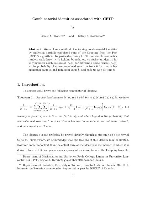
Combinatorial identities associated with CFTP
by
Gareth O. Roberts* and Jeffrey S. Rosenthal**
Abstract. We explore a method of obtaining combinatorial identities
by analysing partially-completed runs of the Coupling from the Past
(CFTP) algorithm. In particular, using CFTP for simple symmetric
random walk (ssrw) with holding boundaries, we derive an identity involving
linear combinations of C ab (s) for different a and b, where C ab (s)
is the probability that unconstrained ssrw run from 0 for time n has
maximum value a, and minimum value b, and ends up at s at time n.
1. Introduction.
This paper shall prove the following combinatorial identity:
Theorem 1.
1
N + 1 =
N ∑
For any fixed integers N, n, and i with 0 < n ≤ N and 0 ≤ i ≤ N, we have
N∑
N−l
∑
k=0 l=0 m=0
[
l
N + 1 1 j=i +
m
N + 1 1 k=i + 1 ]
N + 1 1 k≤i≤j C l,−m (k − m) , (1)
where j ≡ j(k, l, m) ≡ k + N − min(N, l + m), and where C ab (s) is the probability that
unconstrained ssrw run from 0 for time n has maximum value a, and minimum value b,
and ends up at s at time n.
The identity (1) can probably be proved directly, though it appears to be non-trivial
to do so. Furthermore, we acknowledge that applications of this identity may be limited.
However, more important than the actual form of the identity is the manner in which it is
derived. Indeed, (1) emerges as a consequence of the correctness of the Coupling from the
* Department of Mathematics and Statistics, Fylde College, Lancaster University, Lancaster,
LA1 4YF, England. Internet: g.o.robert@lancaster.ac.uk.
** Department of Statistics, University of Toronto, Toronto, Ontario, Canada M5S 3G3.
Internet: jeff@math.toronto.edu. Supported in part by NSERC of Canada.
1

Past (CFTP) algorithm for a very simple Markov chain – the case of constrained simple
symmetric random walk on {0, 1, . . . , N}.
Since CFTP can be applied to essentially any ergodic Markov chain, it appears that
similar (though more complicated) methods could be used to derive other combinatorial
identities, using other Markov chains in other settings (e.g. for the Ising model, as in Propp
and Wilson, 1996).
We explain the CFTP algorithm in Section 2. In Section 3, we explain how CFTP
gives rise to combinatorial identities. We derive the identity (1) in Sections 4 and 5.
Further remarks about the quantities C ab (j), and how to compute them, are presented in
Section 6.
2. Coupling from the Past (CFTP).
Markov chain Monte Carlo (MCMC) algorithms are an extremely popular tool in
statistics to approximately sample from a probability distribution π(·), by designing a
Markov chain P (x, ·) such that π is stationary for P (see e.g. Smith and Roberts, 1993;
Tierney, 1994; Gilks, Richardson, and Spiegelhalter, 1996).
More recently, Propp and Wilson (1996) have developed an algorithm called Coupling
from the Past (CFTP), which makes use of the Markov chain P in a novel way to sample
from π exactly. This has led to an explosion of research in this area; see e.g. Thönnes
(2000) and the multitude of papers described in Wilson (1998).
To define CFTP, let us assume that we have an ergodic Markov chain {X n } n∈Z with
transition kernel P (x, ·) on a state space X , and a probability measure π on X , such that
π is stationary for P (i.e. (πP )(dy) ≡ ∫ π(dx) P (x, dy) = π(dy)). Let us further assume
X
that we have defined the Markov chain as a stochastic recursive sequence, so there is a
function φ : X × R → X and an i.i.d. sequence of random variables {U n } n∈Z , such that
we always have X n+1 = φ(X n , U n ). (It is not strictly necessary to use stochastic recursive
sequences to define CFTP, see e.g. Murdoch and Rosenthal, 2000. On the other hand, it is
easiest, and most common, to define CFTP in this way. Furthermore, the use of stochastic
recursive sequences involves essentially no loss of generality, cf. Borovkov and Foss, 1992.)
CFTP involves considering negative times n, rather than positive times. Specifically,
2

let
φ (n) (x; u −n , . . . , u −1 ) = φ(φ(φ(. . . φ(x, u −n ), u −n+1 ), u −n+2 ), . . .), u −1 ) . (2)
Then CFTP proceeds by considering various increasing choices of T > 0, in the search for
a value T > 0 such that
φ (T ) (x; U −T , . . . , U −1 ) does not depend on x ∈ X , (3)
i.e. such that the chain has coalesced in the time interval from time −T to time 0.
Once such a T has been found, the resulting value
W ≡ φ (T ) (x; U −T , . . . , U −1 )
(which does not depend on x) is the output of the algorithm. Note in particular that,
because of the backward composition implicit in (2), W = φ (n) (y; U −n , . . . , U −1 ) for any
n ≥ T and any y ∈ X . In particular, letting n → ∞, it follows by ergodicity that W ∼ π(·).
(See Propp and Wilson, 1996, for a formal proof of this.)
Note that the values {U n } should be thought of as being fixed in advance, even though
of course they are only computed as needed. In particular, crucially, all previously-used
values of {U n } must be used again, unchanged, as T is increased.
In the special case in which φ is monotone, meaning that there is an ordering ≼
on X such that φ(x, u) ≼ φ(y, u) whenever x ≼ y (which implies that P is stochastically
monotone), and there are maximal and minimal elements x max , x min ∈ X , then to check (3)
it suffices to check that
φ (T ) (x min ; U −T , . . . , U −1 ) = φ (T ) (x max ; U −T , . . . , U −1 ) . (4)
3

3. Identities arising from CFTP.
As mentioned above, CFTP does a search for a value of T satisfying (3), by checking
increasing values of T (often simply doubling the value of T each time) until (3) is satisfied.
Suppose in particular that some fixed value of T has been tried, so that the values
U −T , . . . , U −1 have been generated, and the paths {φ (n) (x, ; U −n , . . . , U −1 )} 1≤n≤T
have
been computed (and perhaps even displayed), though coalescence may have occured by
then. Conditional on the values U −T , . . . , U −1 , the output value W will have some conditional
distribution. Since overall W ∼ π(·), we must have from the Law of Total Probability
that
∫
∫
. . .
P(U −1 ∈ du −1 , . . . , U −T ∈ du −T ) P(W ∈ A | U −1 = u −1 , . . . , U −T = u −T ) = π(A) .
Now, P(W ∈ A | U −1 = u −1 , . . . , U −T = u −T ) could be computed as
P(W ∈ A | U −1 = u −1 , . . . , U −T = u −T ) = P(φ (T ) (X −T ; U −1 , . . . , U −T ) ∈ A) , (5)
except that X −T is unknown. On the other hand, given the values of {U n }, suppose we
choose S > T large enough that φ (S−T ) (x; U −S , . . . , U −S+T −1 ) does not depend on x ∈ X ,
i.e. that coalescence occurs during the time interval from time −S to time −S + T . Let
Z = φ (S−T ) (x; U −S , . . . , U −S+T −1 ) (which does not depend on x). Then, by the validity
of CFTP, we see that Z ∼ π(·). Also, by construction,
φ (S) (x; u −S , . . . , u −1 ) = φ (T ) (φ (S−T ) (x; u −S , . . . , u −T −1 ); u −T , . . . , u −1 )
= φ (T ) (Z; u −T , . . . , u −1 ) .
This suggests that in (5), we can assume that X −T = Z ∼ π(·). The following result
confirms this.
Theorem 2. Consider any CFTP algorithm as described above. Then for any T ∈ N,
∫
∫
. . .
P(U −1 ∈ du −1 , . . . , U −T ∈ du −T ) π{x ∈ X ; φ (T ) (x; u −1 , . . . , u −T ) ∈ A} = π(A) .
(6)
4

Proof. This follows immediately from the stationarity of π, since all says is that if we
start a Markov chain in stationarity at time −T , then it will still be in stationarity at
time 0.
Remark. The proof of Theorem 2 shows that the result does not really depend on CFTP
at all, just on the stationarity of π(·) for the Markov chain. However, it was CFTP that
led us to consider these identities, and provides the proper context for them.
In principle, (6) gives a separate identity for every single Markov chain. The difficulty
lies in interpreting (6) in a way that is meaningful and insightful. To do this, it is necessary
to consider particular Markov chains.
4. The case of ssrw on {0, . . . , N}.
Consider simple symmetric random walk (ssrw) on X = {0, . . . , N}, with holding
boundaries. That is, let {U n } n∈Z be i.i.d., with P(U n = +1) = P(U n = −1) = 1 2 , and
define a Markov chain by
X n+1 = max [ 0, min[N, X n + U n ] ] . (7)
As a stochastic recursive sequence, we can write this as X n+1 = φ(X n , U n ), where
φ(x, u) = max [ 0, min[N, x + u] ] .
This Markov chain has as its stationarity distribution the uniform distribution on X ,
so that π(x) = 1/(N + 1) for x ∈ X . (Indeed, the chain is reversible with respect to π(·),
and in fact it may be regarded as a Metropolis algorithm for π(·) with proposal given by
unconstrained ssrw.) Hence, we can run CFTP for this Markov chain, to output a value
W ∼ π(·). See Rosenthal (1998) for an interactive display of CFTP for this Markov chain,
which illustrates the status of the algorithm after a particular choice of T has been tried
but coalescence has not been achieved.
Note that this chain is indeed monotone, with maximal and minimal values x max = N
and x min = 0. Hence, to check for coalescence we need only check (4). Thus, we consider
just the “bottom process” starting at 0, and the “top process” starting at N.
5

We wish to specialise the general identity (6) to this particular case. To do so, we
proceed as follows.
We first define a “hold” for the top or bottom process to be a time such that the chain
remains in the same state. That is, for fixed N, we let
H top
n = # { m; 1 ≤ m ≤ n; φ (n−m) (N; U −n , . . . , U −n+m ) = φ (n−m+1) (N; U −n , . . . , U −n+m−1 ) } ,
and
H bot
n = # { m; 1 ≤ m ≤ n; φ (n−m) (0; U −n , . . . , U −n+m ) = φ (n−m+1) (0; U −n , . . . , U −n+m−1 ) } .
Let R N,n,l,m,k be the probability that the Markov chain given by (7), when run for a
time n, has all of the following properties: (a) the bottom process ends up at k ∈ X ; (b)
the top process has l holds; and (c) the bottom process has m holds. It necessarily follows
from this that (d) the top process ends up at j = j(k, l, m) = k + N − min(N, l + m).
In symbols, if we fix N throughout, then we can write this as
R N,n,l,m,k
= P(φ (n) (0, U −n , . . . , U −1 ) = k, H top
n
= l, H bot
n = m) .
We have the following.
Lemma 3. Consider a partial run of CFTP for ssrw, from time −n to time 0, as above.
Let j ≡ j(k, l, m) ≡ k + N − min(N, l + m). Then if l + m < N (so that j < k), then
and for j < i < k,
P (W = k | φ (n) (0, U −n , . . . , U −1 ) = k, H top
n
P (W = j | φ (n) (0, U −n , . . . , U −1 ) = k, H top
n
= l, H bot
n = m) = l + 1
N + 1 ,
= l, H bot
n = m) = m + 1
N + 1 ,
P (W = i | φ (n) (0, U −n , . . . , U −1 ) = k, H top
n
= l, H bot
n = m) =
1
N + 1 .
If instead l + m = N, so that j = k, then
P (W = k | φ (n) (0, U −n , . . . , U −1 ) = k, H top
n
6
= l, H bot
n = m) = 1 .

Proof. As in the proof of Theorem 2, we may assume (either by extending the CFTP
construction back far enough, or by simply using stationarity of π) that the run {X t } is
already in stationarity at time −n.
Now, from time −n to 0, assuming the processes have not yet coalesced, then every
time the top process holds, the process {X t } moves one unit closer to the top process.
Similarly, every time the bottom process holds, the process {X t } moves one unit closer to
the bottom process. It follows that X 0 = j if and only if X −n ≥ N − l, and X 0 = k if
and only if X −n ≤ m. Otherwise, the values of X −n strictly between m and N − l are in
a one-one correspondence with the values of X 0 strictly between k and j.
Hence, if l + m < N so that j < k, then
and
P (W = k | φ (n) (0, U −n , . . . , U −1 ) = k, H top
n
= l, H bot
n = m) = P (X −n ≤ m) ,
P (W = j | φ (n) (0, U −n , . . . , U −1 ) = k, H top
n
while for j < i < k,
= l, H bot
n = m) = P (X −n ≥ N − l) ,
P (W = i | φ (n) (0, U −n , . . . , U −1 ) = k, H top
n
Since X −n ∼ π(·), the result for the case j < k follows.
On the other hand, if l + m = N so that j = k, then
= l, H bot
n = m) = P (X −n = m − k + i) .
P (W = k | φ (n) (0, U −n , . . . , U −1 ) = k, H top
n
thus establishing the result in the case l + m = N as well.
= l, H bot
n = m) = P (X −n ∈ X ) = 1 ,
Using this lemma and the definition of R N,n,l,m,k , we see that Theorem 2 can now be
written as follows. (For the case l + m = N, we use the observation that if i = j = k, then
l
N+1 1 j=i + m
N+1 1 k=i + 1
N+1 1 k≤i≤j = 1.)
7

Proposition 4.
For fixed integers N, n, and i, with 0 < n ≤ N and 0 ≤ i ≤ N, letting
j = j(k, l, m) = k + N − min(N, l + m), we have the identity
1
N + 1 =
N ∑
k=0
∑
l,m≥0
m+l≤n
[
l
N + 1 1 j=i +
m
N + 1 1 k=i + 1 ]
N + 1 1 k≤i≤j R N,n,l,m,k .
5. Interpreting the quantities R N,n,l,m,k .
To clarify the result of Proposition 4, we wish to better interpret the quantities
R N,n,l,m,k . Fix N, n ∈ N throughout. We first note the following.
Proposition 5. If l + m ≤ N, then R N,n,l,m,k is equal to the probability that unconstrained
ssrw starting at 0 and run for time n, has maximum value l, minimum value −m,
and ends up at k − m. In symbols,
R N,n,l,m,k = C l,−m (k − m) ,
where
[
C ab (s) = P max Z t = a,
0≤t≤n
]
min Z t = b, Z n = s ,
0≤t≤n
where {Z t } is unconstrained ssrw started at 0 and run for time n.
Proof. Consider running CFTP as described above, using random variables U −n , . . . , U −1 .
Let Z 0 = 0, and Z t = U −n + . . . + U −n+t−1 for 0 < t ≤ n. Then {Z t } is indeed equal to
an unconstrained ssrw started at 0 and run for time n. However, it has now been coupled
with the CFTP algorithm under consideration, and we shall make use of this fact.
Now, suppose that for the CFTP algorithm, the event whose probability is R N,n,l,m,k
has indeed occurred. That is, suppose that the bottom process of CFTP ends up at k, the
top process has l holds, and the bottom process has m holds. We wish to see what effect
these suppositions have on the unconstrained process {Z t }.
Let −s be the time just after the last hold of the bottom process of the CFTP algorithm.
Then the corresponding value of the {Z t } process, namely Z n−s , must be equal to
−m. Furthermore, we will then have Z t ≥ −m for all t ≥ n − s. It follows that we will
have min 0≤t≤n Z t = −m. Similarly, we will have max 0≤t≤n Z t = −m.
8

Finally, the value of Z n must be equal to the value of the bottom process in the
CFTP algorithm, minus the number of times the bottom process held at 0 (so that it
didn’t decrease, even though {Z t } did). Hence, we must have Z n = k − m.
Conversely, it is easily checked that if min 0≤t≤n Z t = −m, and max 0≤t≤n Z t = −m,
and Z n = k − m, then it must be that the bottom process of CFTP ends up at k, the top
process has l holds, and the bottom process has m holds.
We conclude that
R N,n,l,m,k
= P( min
0≤t≤n Z t = −m ,
max Z t = −m , Z n = k − m) .
0≤t≤n
This gives the result.
Combining Proposition 5 with Proposition 4, we immediately obtain Theorem 1.
Remark.
If l + m > N, then it is possible that the bottom process will actually reach
the top value of N, and then hold at the top value. This implies that the final value of
the corresponding unconstrained ssrw will no longer be just a function of k, l, m, which
causes additional complications. It is possible to overcome these complications, however
to do so is somewhat messy and not particularly useful. Hence, in the above proposition,
we restrict to the case l + m ≤ N. In Theorem 1, we restrict to the case n ≤ N, precisely
so that these additional complications do not arise.
6. Computing the quantities C ab (s).
In order to verify the result of Theorem 1 numerically (say), it is necessary to know
how to compute the quantities C ab (s). The reflection principle for ssrw is of some help
here. However, since the events corresponding to C ab (s) specify both a maximum value
and a minimum value, it seems that the best we can do is compute C ab (s) in terms of a
sum of O(n) terms. We present that here.
To begin, let
Q n (x) =
⎧
⎪⎨
⎪⎩
( ) n
2 −n n+x
, − n ≤ x ≤ n, x + n even
2
0 , otherwise
9

e the probability that unconstrained ssrw on the set of all integers, starting from 0, is at
the point x at time n.
Now, for any integers x 1 , x 2 , . . . , x r , j, let A x1 x 2 ...x r
(j) be the probability that unconstrained
ssrw, starting from 0 and run for time n, hits in turn the values x 1 , x 2 , . . . , x r ,
and then ends up at j at time n. Also, say a sequence x 1 , x 2 , . . . , x r is sign alternating if
(x q − x q−1 )(x q+1 − x q ) ≤ 0 for 2 ≤ q ≤ r − 1.
Lemma 6. If the sequence x 1 , x 2 , . . . , x r , j is sign-alternating, then
A x1 x 2 ...x r
(j) = Q n (|x 1 | + |x 2 − x 1 | + . . . + |x r − x r−1 | + |j − x r |) .
Proof. Just use the reflection principle for ssrw, r times (cf. pp. 72, 96 of Feller, 1968).
Now let B ab (j) be the probability that unconstrained ssrw hits run from time 0 to n,
hits both a and b, and furthermore ends up at j at time n.
Lemma 7. We always have B 00 (j) = 0. Otherwise, for (a, b) ≠ (0, 0) and ab ≤ 0,
B ab (j) = [A ab (j) − A aba (j) + A abab (j) − A ababa (j) + . . .]
+ [A ba (j) − A bab (j) + A baba (j) − A babab (j) + . . .] .
(Since A x1 x 2 ...x r
(j) = 0 whenever |x 1 | + |x 2 − x 1 | + . . . + |x r − x r−1 | > n, the above sums
each terminate after at most n/|b − a| terms.)
Proof.
By the inclusion-exclusion principle, the probability that we first hit b, and then
hit a, finally ending up at j, is equal to
A ab (j) − A bab (j) + A abab (j) − A babab (j) + . . . .
Similarly, the probability that we first hit a, and then hit b, finally ending up at j, is equal
to the same sum but with a and b reversed. Adding these two sums, we obtain the formula
for B ab (j) as claimed.
10

Remark.
Note that we cannot compute B ab (j) in simple closed form, as
[A ab (j) − A bab (j)] + [A ba (j) − A aba (j)] .
The problem with this is that paths of the form abab would end up getting added and
subtracted equally often, and therefore counted a total of zero times, rather than one time
as desired.
Now recall that C ab (j) is the probability that unconstrained ssrw has maximum value
a, and minimum value b, and ends up at j at time n.
Lemma 8. For a ≥ 0 ≥ b,
C ab (j) = B ab (j) − B a+1,b (j) − B a,b−1 (j) + B a+1,b−1 (j) .
Proof. B ab (j) is the probability that the max is at least a and the min is at most b
(and we end up at j). The formula then follows from the basic probability result that
P(A 1 ∩ A C 2 ∩ A C 3 ) = P(A 1 ) − P(A 1 ∩ A 2 ) − P(A 1 ∩ A 3 ) + P(A 1 ∩ A 2 ∩ A 3 ), where
A 1 = {max ≥ a , min ≤ b}, A 2 = {max ≥ a + 1}, A 3 = {min ≤ b − 1}.
The above three lemmas together provide a fully computable formula for R N,n,l,m,j ,
whenever l + m ≤ N. This allows us to numerically verify the identity (1), for any appropriate
choices of N, n, and i. Such verification has been done in the C program combin.c,
freely available at http://markov.utstat.toronto.edu/jeff/comp/combin.c
The three lemmas also allow the possibility of analytically expanding the identity of
Theorem 1 further, in an effort to simplify or better understand it. However, it is not clear
that such an expanded version provides any helpful new insights, so we do not pursue it
here.
11

REFERENCES
A.A. Borovkov and S.G. Foss (1992), Stochastically recursive sequences and their
generalizations. Siberian. Adv. Math. 2, 16–81.
S.P. Brooks (1998), Markov Chain Monte Carlo Method and its Application. The
Statistician 47, 69–100.
W. Feller (1968), An Introduction to Probability Theory and its Applications, Volume
I (3 rd ed.). Wiley, New York.
W.R. Gilks, S. Richardson, and D.J. Spiegelhalter, eds. (1996), Markov chain Monte
Carlo in practice. Chapman and Hall, London.
D.J. Murdoch and P.J. Green (1998), Exact sampling from a continuous state space.
Scandinavian Journal of Statistics 25(3), 483–502.
D.J. Murdoch and J.S. Rosenthal (2000), “Efficient use of exact samples”. Statistics
and Computing 10, 237–243.
J.G. Propp and D.B. Wilson (1996). Exact sampling with coupled Markov chains and
applications to statistical mechanics. Random Structures and Algorithms 9, 223–252.
J.S. Rosenthal (1998). CFTP Java Applet. Available at
http://markov.utstat.toronto.edu/jeff/java/cftp.html
A.F.M. Smith and G.O. Roberts (1993), Bayesian computation via the Gibbs sampler
and related Markov chain Monte Carlo methods (with discussion). J. Roy. Stat. Soc. Ser.
B 55, 3-24.
E. Thönnes (2000), A primer on perfect simulation. In Statistical Physics and Spatial
Statistics (K.R. Mecke and D. Stoyan, eds.), Springer Lecture Notes in Physics, volume
554, 349–378.
L. Tierney (1994), Markov chains for exploring posterior distributions (with discussion).
Ann. Stat. 22, 1701-1762.
D.B. Wilson (1998). Annotated bibliography of perfectly random sampling with Markov
chains. Available at http://dimacs.rutgers.edu/∼dbwilson/exact/
12