Potential Output: Concepts and Measurement - Department of Labour

Darren Gibbs 99
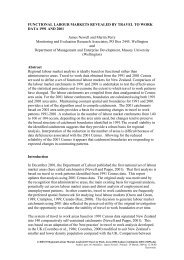
FIGURE 7: Estimated potential output and output gap series—bivariate filter
method
20
15
10000
Output gap (%)
10
5
0
-5
-10
-15
-20
8000
6000
4000
2000
0
1977
1978
1979
1980
1981
1982
1983
1984
1985
1986
1987
1988
1989
1990
1991
1992
1993
Output ($m 82/83)
June years
bf200: output gap (left axis)
bf100,000: output gap (left axis)
bf200: potential output (right axis)
bf100,000: potential output (right axis)
bf1600: output gap (left axis)
gdp (right axis)
bf1600: potential output (right axis)
contained in this regression was than embedded within the Hodrick-Prescott
minimisation formula to yield a bivariate estimate of potential output which was
based on both the observed behaviour of output and the observed behaviour of
inflation. Next, the Phillips curve was re-estimated with the initial Hodrick-
Prescott derived output gap being replaced by the new estimated bivariate
output gap. The bivariate filter was then re-estimated using the information from
this updated regression. This iterative procedure was repeated until the
coefficients in the re-estimated Phillips curve converged.
As noted in section 3, the procedure can be generalised to allow independently
determined weights to be placed on the various terms in the minimisation
problem. This facility was used so as to effectively give zero weight to developments
in inflation during the 1982–84 wage and price freeze, and to the 1986 and
1989 GST induced increases in indirect tax.
As with the potential output estimates derived using the pure Hodrick-
Prescott approach three variations of the smoothness parameter were used, so
that three different bivariate filters were derived. Figure 7 illustrates the three
estimated potential output series (bf1600, bf200, bf100,000) obtained by following
the above approach, and the estimated output gaps.