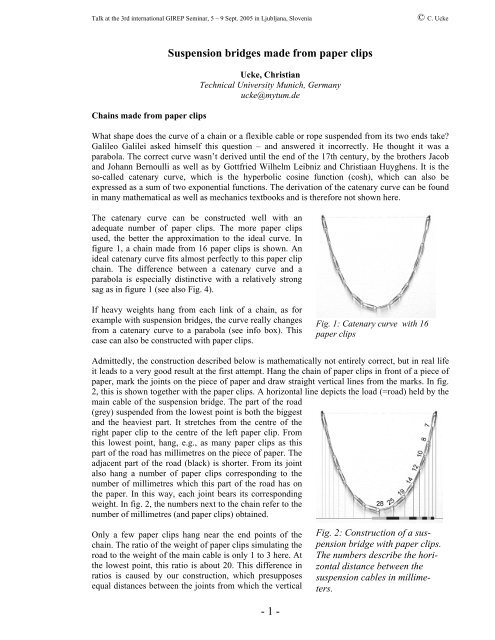
Suspension bridges with paper clips

Talk at the 3rd international GIREP Seminar, 5 – 9 Sept. 2005 in Ljubljana, Slovenia
© C. Ucke
Chains made from paper clips
Suspension bridges made from paper clips
Ucke, Christian
Technical University Munich, Germany
ucke@mytum.de
What shape does the curve of a chain or a flexible cable or rope suspended from its two ends take?
Galileo Galilei asked himself this question – and answered it incorrectly. He thought it was a
parabola. The correct curve wasn’t derived until the end of the 17th century, by the brothers Jacob
and Johann Bernoulli as well as by Gottfried Wilhelm Leibniz and Christiaan Huyghens. It is the
so-called catenary curve, which is the hyperbolic cosine function (cosh), which can also be
expressed as a sum of two exponential functions. The derivation of the catenary curve can be found
in many mathematical as well as mechanics textbooks and is therefore not shown here.
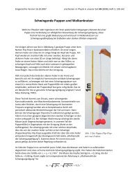
The catenary curve can be constructed well with an
adequate number of paper clips. The more paper clips
used, the better the approximation to the ideal curve. In
figure 1, a chain made from 16 paper clips is shown. An
ideal catenary curve fits almost perfectly to this paper clip
chain. The difference between a catenary curve and a
parabola is especially distinctive with a relatively strong
sag as in figure 1 (see also Fig. 4).
If heavy weights hang from each link of a chain, as for
example with suspension bridges, the curve really changes
from a catenary curve to a parabola (see info box). This
case can also be constructed with paper clips.
Fig. 1: Catenary curve with 16
paper clips
Admittedly, the construction described below is mathematically not entirely correct, but in real life
it leads to a very good result at the first attempt. Hang the chain of paper clips in front of a piece of
paper, mark the joints on the piece of paper and draw straight vertical lines from the marks. In fig.
2, this is shown together with the paper clips. A horizontal line depicts the load (=road) held by the
main cable of the suspension bridge. The part of the road
(grey) suspended from the lowest point is both the biggest
and the heaviest part. It stretches from the centre of the
right paper clip to the centre of the left paper clip. From
this lowest point, hang, e.g., as many paper clips as this
part of the road has millimetres on the piece of paper. The
adjacent part of the road (black) is shorter. From its joint
also hang a number of paper clips corresponding to the
number of millimetres which this part of the road has on
the paper. In this way, each joint bears its corresponding
weight. In fig. 2, the numbers next to the chain refer to the
number of millimetres (and paper clips) obtained.
Only a few paper clips hang near the end points of the
chain. The ratio of the weight of paper clips simulating the
road to the weight of the main cable is only 1 to 3 here. At
the lowest point, this ratio is about 20. This difference in
ratios is caused by our construction, which presupposes
equal distances between the joints from which the vertical
Fig. 2: Construction of a suspension
bridge with paper clips.
The numbers describe the horizontal
distance between the
suspension cables in millimeters.
- 1 -

Talk at the 3rd international GIREP Seminar, 5 – 9 Sept. 2005 in Ljubljana, Slovenia
© C. Ucke
cables hang. With real suspension bridges, the horizontal
distances of the vertical cables are the same. The – constant
– weight ratio is between about 10 to 1 and 15 to 1. Since
there is no ideal weightless main cable, the shape of a real
main cable is a mixture of a catenary and a parabola. In
reality, this does not pose a problem for the design
engineers, because a small sag makes the difference between
a catenary and a parabola negligible.
The shape of the curve in figure 3 is that of an ideal parabola
to within a very small margin of error.
With physics simulation programs like Interactive Physics
[1] or XYZet [2] you can also very nicely illustrate the
situations described above. In figure 4, you can see the
simulation of a catenary curve with 16 unweighted links
(grey line) and a 'suspension bridge' equipped with
corresponding weights (black parabola), both superimposed
on one another. With a real suspension bridge, the vertical
suspender cables are equidistant from one another (this can
also be simulated with the program). In figure 4, however,
the points on the main suspension cable where the vertical
suspender cables are fastened are equidistant from one
another.
Fig. 3: Parabola with 16 clips and
weights. The complete weights with
the clip chains are not shown here.
In the WEB you can find many links under the term
‘catenary curve’, and also historical remarks and derivations.
Furthermore, there are very descriptive applets that clarify
the difference between the catenary curve and the parabola.
Info-box (suspension bridge parabola)
Overly simplified and idealized, the form of the curve of the
main cable of a suspension bridge can be derived in the
following way:
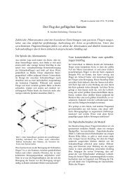
Three forces, whose vectorial sum must yield exactly zero
(figure 5), act in a point P of the main cable of a suspension
bridge. First, the force G of a part of the road with the
length x acts vertically downward. Secondly, a
horizontal force S is exerted by the tension of the
cable. This force is constant over the whole cable.
Thirdly, a force F acts in the direction of the tangent to
the cable. This tangential force corresponds exactly to
the slope at point P.
Let’s take µ as the weight per unit of length of the
roadway suspended at the cable. The coordinate origin
0 is located at the vertex of the curve. The weight G
acting at the point P is then exactly G = µ·x. If we
denote the height of the cable at the point x by y, then
the slope at this point is
- 2 -
Fig. 4: Simulation of a catenary
curve (grey) and a parabola
(black) using ‘Interactive Physics’
y
0
suspended roadway
Fig. 5: A parabola emerges as a curve
form for the main cable of a suspension
bridge.
G
x
S
F
S
P
G
F
x

Talk at the 3rd international GIREP Seminar, 5 – 9 Sept. 2005 in Ljubljana, Slovenia
© C. Ucke
y′
=
G
S
µ ⋅ x
=
S
By integrating this equation we get
µ ⋅ x µ 2
y = ∫ dx = x + C
S 2S
Since the origin 0 of the curve is located at the vertex, the integration constant is C = 0 .
Consequently, the curve is a parabola.
References:
[1] http://www.interactivephysics.com/ (in English)
[2] http://www.ipn.uni-kiel.de/persons/michael/xyzet/ (in English)
- 3 -