Problem Set 5, Jeremy Lise - UCL
Problem Set 5, Jeremy Lise - UCL
Problem Set 5, Jeremy Lise - UCL

You also want an ePaper? Increase the reach of your titles
YUMPU automatically turns print PDFs into web optimized ePapers that Google loves.
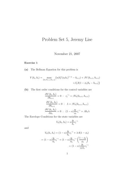
<strong>Problem</strong> <strong>Set</strong> 5, <strong>Jeremy</strong> <strong>Lise</strong><br />
November 21, 2007<br />
Exercise 1<br />
(a)<br />
The Bellman Equation for this problem is<br />
(b)<br />
V (k t , h t ) =<br />
max<br />
{φ t,h t+1 ,k t+1 } {u(kα t (φ t h t ) 1−α − k t+1 ) + βV (k t+1 , h t+1 )<br />
+λ[A(1 − φ t )h t − h t+1 ]}<br />
The first order conditions for the control variables are<br />
∂V (k t , h t )<br />
∂k t+1<br />
= 0 : c −γ<br />
t = βV k (k t+1 , h t+1 )<br />
∂V (k t , h t )<br />
= 0 : λ = βV h (k t+1 , h t+1 )<br />
∂h t+1<br />
∂V (k t , h t )<br />
= 0 : (1 − α) y t<br />
c −γ<br />
t = Ah t λ<br />
∂φ t φ t<br />
The Envelope Conditions for the state variables are<br />
and<br />
V k (k t , h t ) = α y t<br />
c −γ<br />
t<br />
k t<br />
V h (k t , h t ) = (1 − α) y t<br />
c −γ<br />
t + λA(1 − φ t )<br />
h t<br />
= (1 − α) y t<br />
c −γ<br />
t + (1 − α) y ( )<br />
t 1 −<br />
c −γ φt<br />
t<br />
h t h t φ t<br />
1<br />
= (1 − α) y t<br />
c −γ<br />
t<br />
φ t h t
Use the Envelope Condition for k t in the first order condition for consumption<br />
to get the standard consumption Euler Equation<br />
( )<br />
c −γ yt+1<br />
t = αβ c −γ<br />
t+1 (1)<br />
k t+1<br />
Combine the first order conditions for φ t and h t+1 and use the Envelope<br />
Condition for h t to get the Euler Equation for human capital<br />
y t+1<br />
(1 − α) y t<br />
c −γ<br />
t = Ah t β(1 − α) c −γ<br />
φ t φ t+1 h t+1<br />
c −γ<br />
t<br />
= Aβ<br />
(<br />
yt+1<br />
y t<br />
t+1<br />
) (<br />
φt<br />
φ t+1<br />
) (<br />
ht<br />
h t+1<br />
)<br />
c −γ<br />
t+1 (2)<br />
(c) Along a balanced growth path (BGP) human capital h t grows at a<br />
constant rate g h . From the production function for human capital we have<br />
1 + g h = A(1 − φ t )<br />
But as the left hand side of the equation is constant, so is the right hand<br />
side. It follows that along a BGP, φ t = φ is constant.<br />
(d) First consider equation (1)<br />
( ) γ ct+1<br />
= (1 + g c ) γ = αβ<br />
c t<br />
(<br />
yt+1<br />
k t+1<br />
)<br />
For g c to be constant along a BGP, the ratio y t+1 /k t+1 has to be constant.<br />
But this implies g y = g k .<br />
Now divide the resource constraint by k t<br />
c t<br />
k t<br />
= y t<br />
k t<br />
− k t+1<br />
k t<br />
= y t<br />
k t<br />
− (1 + g k )<br />
Along a BGP the right hand side has to be constant, so the ratio c t /k t has<br />
to be constant, i.e. g c = g k .<br />
Finally, divide the consumption goods production function by k t<br />
( ) α ( ) 1−α ( ) 1−α<br />
y t kt<br />
= φ 1−α ht<br />
= φ 1−α ht<br />
k t k t k t k t<br />
2
As g y = g k , it follows from this equation that g h = g k .<br />
This establishes that g h = g k = g h = g.<br />
In a last step we will solve for g. Take (2) along the BGP<br />
( ) ( )<br />
φ 1<br />
(1 + g) γ = Aβ(1 + g)<br />
= Aβ<br />
φ 1 + g<br />
It follows that<br />
Exercise 3<br />
g = (Aβ) 1/γ − 1<br />
(a) As only households can hold bonds, in equilibrium aggregate bonds<br />
need to be zero, i.e. households’ demand for bonds has to be equal to households’<br />
supply of bonds. However given that all households are the same and<br />
they all face the same aggregate shock, at given prices they all either want to<br />
sell bonds or buy bonds. So in equilibrium (!) for the bond market to clear,<br />
individual bond holdings have to be zero ( B t = 0 ) in ever period. But this<br />
implies that the transversality condition for bonds holds trivially.<br />
(a) Let’s solve the household problem first. The households will chose<br />
current and future consumption and labor supply in order to maximize its<br />
intertemporal utility function subject to its budget constraint, taking prices<br />
as given.<br />
The Bellman equation for the households problem is<br />
[ c<br />
1−θ<br />
]<br />
t<br />
V (B t ) = max<br />
C t,L t 1 − θ − φ L1+η t<br />
1 + η + e−ρ V (W t L t + R t−1 B t−1 − C t )<br />
The first order conditions are<br />
and by the Envelope Condition<br />
C −θ<br />
t = e −ρ V ′ (B t )<br />
φL η t = W t e −ρ V ′ (B t )<br />
V ′ (B t−1 ) = R t−1 e −ρ V ′ (B t ) = R t−1 C −θ<br />
t<br />
3
where I have used the first order condition for consumption.<br />
Combining these three equation we get a labor supply equation for the household<br />
φL η t = W t Ct −θ<br />
(3)<br />
and a consumption Euler Equation<br />
C −θ<br />
t<br />
Together with the household’s budget constraint<br />
= e −ρ R t C −θ<br />
t+1 (4)<br />
W t L t + R t−1 B t−1 = C t + B t (5)<br />
these two equations describe optimal household behavior at given prices.<br />
Now let’s turn to the firm. The firm will maximize profits taking prices<br />
as given. The firm’s profit function is<br />
Π t = e zt N t − W t N t = (e zt − W t )N t<br />
For a given W t the firm’s labor demand is as follows<br />
N t = ∞ for W t < e zt<br />
N t = [0, ∞) for W t = e zt<br />
N t = 0 for W t > e zt<br />
In equilibrium households and the firm will behave optimally given prices,<br />
and all markets clear. We have three markets, the consumption goods market,<br />
the bond market, and the labour market. By Walras’ Law we can ignore<br />
one market clearing condition. Let’s take the consumption goods market.<br />
As seen in (a), bond market clearing requires<br />
Labor market clearing requires<br />
B t = 0 (6)<br />
N t = HL t (7)<br />
But from the firm’s labor demand curve we can see that this immediately<br />
implies<br />
W t = e zt . (8)<br />
Equations (3) to (8) characterize the competitive equilibrium of this economy.<br />
4
(c) Now assume z t = 0 and derive the steady states for W, Y, C, N and R.<br />
First, from (8) we have<br />
W = 1<br />
Using this and B t = 0 we get from (5) that<br />
L = C<br />
Now by (3)<br />
φL η = L −θ ⇒ L =<br />
( 1<br />
φ) 1<br />
η+θ<br />
But this together with the labor market clearing condition (7) gives us steady<br />
state output<br />
( 1<br />
1<br />
η+θ<br />
Y = H<br />
φ)<br />
Finally from the consumption Euler Equation (4) we have<br />
R = e ρ<br />
(d) Now let’s log-linearize equations (3) to (8).<br />
Equation (3) is<br />
φ(e lt L) η = e wt W (e ct C) −θ = φL η e ηlt = W C −θ e wt−θct<br />
Using the steady state definition and taking logs on both sides we get<br />
Equation (4):<br />
l t = 1 η (w t − θc t ) (9)<br />
(e ct C) −θ = e −ρ e rt R(e c t+1<br />
C) −θ<br />
Again using the steady state of R we get<br />
c t+1 − c t = 1 θ (r t − ρ) (10)<br />
Equation (5): Use the equilibrium condition B t = 0. Then<br />
e wt W e lt L = e ct C<br />
5
Equation (7):<br />
Equation (8):<br />
Finally output is<br />
c t = w t + l t<br />
e nt N = He lt L<br />
n t = l t (11)<br />
e wt W = e zt<br />
w t = z t (12)<br />
e y t Y = e zt Ne nt<br />
y t = z t + n t (13)<br />
(e)<br />
Using the budget constraint and w t = z t we have<br />
c t = z t + l t<br />
Now plug this into the labor supply equation<br />
ηl t = z t − θ(z t + l t )<br />
It follows that labor is<br />
l t =<br />
( ) 1 − θ<br />
z t (14)<br />
θ + η<br />
Now use the budget constraint again to get c t<br />
( ) 1 + η<br />
c t = z t (15)<br />
θ + η<br />
Output in this model has to be equal to consumption as there is no investment<br />
( ) 1 + η<br />
y t = z t (16)<br />
θ + η<br />
Finally the interest rate is<br />
[ ] θ(1 + η)<br />
r t = ρ + θ(c t+1 − c t ) = ρ +<br />
(z t+1 − z t )<br />
θ + η<br />
6
where<br />
[ ] θ(1 + η)<br />
r t = ρ +<br />
e t+1 −<br />
θ + η<br />
z t+1 = αz t + e t+1<br />
1<br />
[ θ(1 + η)(1 − α)<br />
θ + η<br />
]<br />
z t (17)<br />
To derive the variances, note that Var(z t ) = σ 2 /(1 − α 2 ). So<br />
Var(w t ) =<br />
σ2<br />
1 − α 2<br />
( ) 2 1 − θ σ 2<br />
Var(l t ) =<br />
θ + η 1 − α 2<br />
( ) 2 1 + η σ 2<br />
Var(c t ) = Var(y t ) =<br />
θ + η 1 − α 2<br />
{ [θ(1 ] 2 [ ] 2 ( ) } + η) θ(1 + η)(1 − α) 1<br />
Var(r t ) =<br />
+<br />
σ 2<br />
θ + η<br />
θ + η 1 − α 2<br />
(f) Real wage are procyclical in the model whereas they a acyclical in the<br />
data.<br />
Hours worked and productivity ( here z t ) are positively correlated in the<br />
model, but are uncorrelated or slightly negatively correlated in the data.<br />
Hours worked fluctuate less than output and consumption in the model (<br />
−θ < η ), but are as volatile as output in the data, and more volatile than<br />
consumption.<br />
Output is as volatile as consumption in the model, but is more volatile than<br />
consumption in the data.<br />
1 I have changed notation here so as not to confound the persistence of the shock with<br />
the time discount factor.<br />
7