Evaluation of structural natural frequencies using image processing
Evaluation of structural natural frequencies using image processing
Evaluation of structural natural frequencies using image processing

You also want an ePaper? Increase the reach of your titles
YUMPU automatically turns print PDFs into web optimized ePapers that Google loves.
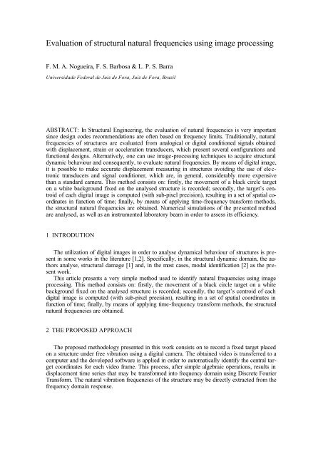
<strong>Evaluation</strong> <strong>of</strong> <strong>structural</strong> <strong>natural</strong> <strong>frequencies</strong> <strong>using</strong> <strong>image</strong> <strong>processing</strong><br />
F. M. A. Nogueira, F. S. Barbosa & L. P. S. Barra<br />
Universidade Federal de Juiz de Fora, Juiz de Fora, Brazil<br />
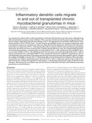
ABSTRACT: In Structural Engineering, the evaluation <strong>of</strong> <strong>natural</strong> <strong>frequencies</strong> is very important<br />
since design codes recommendations are <strong>of</strong>ten based on frequency limits. Traditionally, <strong>natural</strong><br />
<strong>frequencies</strong> <strong>of</strong> structures are evaluated from analogical or digital conditioned signals obtained<br />
with displacement, strain or acceleration transducers, which present several configurations and<br />
functional designs. Alternatively, one can use <strong>image</strong>-<strong>processing</strong> techniques to acquire <strong>structural</strong><br />
dynamic behaviour and consequently, to evaluate <strong>natural</strong> <strong>frequencies</strong>. By means <strong>of</strong> digital <strong>image</strong>,<br />
it is possible to make accurate displacement measuring in structures avoiding the use <strong>of</strong> electronic<br />
transducers and signal conditioner, which are, in general, considerably more expensive<br />
than a standard camera. This method consists on: firstly, the movement <strong>of</strong> a black circle target<br />
on a white background fixed on the analysed structure is recorded; secondly, the target’s centroid<br />
<strong>of</strong> each digital <strong>image</strong> is computed (with sub-pixel precision), resulting in a set <strong>of</strong> spatial coordinates<br />
in function <strong>of</strong> time; finally, by means <strong>of</strong> applying time-frequency transform methods,<br />
the <strong>structural</strong> <strong>natural</strong> <strong>frequencies</strong> are obtained. Numerical simulations <strong>of</strong> the presented method<br />
are analysed, as well as an instrumented laboratory beam in order to assess its efficiency.<br />
1 INTRODUTION<br />
The utilization <strong>of</strong> digital <strong>image</strong>s in order to analyse dynamical behaviour <strong>of</strong> structures is present<br />
in some works in the literature [1,2]. Specifically, in the <strong>structural</strong> dynamic domain, the authors<br />
analyse, <strong>structural</strong> damage [1] and, in the most cases, modal identification [2] as the present<br />
work.<br />
This article presents a very simple method used to identify <strong>natural</strong> <strong>frequencies</strong> <strong>using</strong> <strong>image</strong><br />
<strong>processing</strong>. This method consists on: firstly, the movement <strong>of</strong> a black circle target on a white<br />
background fixed on the analysed structure is recorded; secondly, the target’s centroid <strong>of</strong> each<br />
digital <strong>image</strong> is computed (with sub-pixel precision), resulting in a set <strong>of</strong> spatial coordinates in<br />
function <strong>of</strong> time; finally, by means <strong>of</strong> applying time-frequency transform methods, the <strong>structural</strong><br />
<strong>natural</strong> <strong>frequencies</strong> are obtained.<br />
2 THE PROPOSED APPROACH<br />
The proposed methodology presented in this work consists on to record a fixed target placed<br />
on a structure under free vibration <strong>using</strong> a digital camera. The obtained video is transferred to a<br />
computer and the developed s<strong>of</strong>tware is applied in order to automatically identify the central target<br />
coordinates for each video frame. This process, after simple algebraic operations, results in<br />
displacement time series that may be transformed into frequency domain <strong>using</strong> Discrete Fourier<br />
Transform. The <strong>natural</strong> vibration <strong>frequencies</strong> <strong>of</strong> the structure may be directly extracted from the<br />
frequency domain response.
2.1 Model and <strong>image</strong> <strong>processing</strong><br />
This paper analyses the dynamic behaviour <strong>of</strong> a cantilever beam through <strong>natural</strong> frequency<br />
evaluation <strong>using</strong> <strong>image</strong> sequences <strong>of</strong> a target placed on the structure. Figure 1 presents the beam<br />
model with a circular target and also shows the global and the <strong>image</strong> coordinate systems adopted<br />
in this paper.<br />
Target<br />
Global<br />
System<br />
Image<br />
System<br />
Y<br />
ϕ<br />
κ<br />
Z<br />
y<br />
Pc<br />
Camera<br />
x<br />
θ<br />
X<br />
Figure 1 - Cantilever beam model, target and coordinate systems.<br />
The camera position was defined by its perspective centre coordinates Pc ( X , Y , Z )<br />
<strong>using</strong> global system as referential, having orientation defined by rotation angles κ (Z axis), ϕ (Y<br />
axis), and θ (X axis).<br />
The target must allow a robust identification through automatic methods and it should present<br />
geometric characteristics compatible to the application. In this way, a black circle on a white<br />
background is used as target.<br />
A simple thresholding is capable to transform a grayscale (8 bits) or true colour (24 bits) <strong>image</strong><br />
into a binary (1 bit) <strong>image</strong> as presented in figure 2 [3]. In this case a grayscale <strong>image</strong> is<br />
transformed into a binary <strong>image</strong>. The thresholding defines the limit between the light and dark<br />
<strong>image</strong> pixel grayscale, transforming light ones into white pixels, and dark ones into black pixels.<br />
Using a binary <strong>image</strong>, the pixels attached to the black colour (inside the circle) have the label<br />
b(x,y)=1, and the pixels attached to the white colour (outside the circle) have the label b(x,y)=0,<br />
as shown in figure 2.<br />
Pc<br />
Pc<br />
Pc
Figure 2 - The threshold operation.<br />
The thresholding limit may be considered constant if the illumination conditions are stable during<br />
all operation.<br />
After the target pixel identification, it is possible to determine the black circle <strong>image</strong> cen-<br />
x , y , shown in figure 2, with sub-pixel precision <strong>using</strong>:<br />
troid ( )<br />
1<br />
x =<br />
N M<br />
and:<br />
1<br />
y =<br />
N M<br />
N<br />
M<br />
∑∑<br />
x= 1 y=<br />
1<br />
N<br />
M<br />
∑∑<br />
x= 1 y=<br />
1<br />
b( x, y)x<br />
.<br />
b( x, y)y<br />
.<br />
(1)<br />
(2)<br />
where:<br />
N and M are the number <strong>of</strong> columns and rows <strong>of</strong> the <strong>image</strong>, respectively.<br />
Normalizing summation <strong>of</strong> b(x,y) to the unit, expressions (1) e (2) may be faced as the first<br />
probability distribution moment <strong>of</strong> b(x,y).<br />
2.2 Time history series and <strong>natural</strong> <strong>frequencies</strong><br />
By taking the coordinates ( x ,y ) obtained for each frame, it is possible to generate time history<br />
series x and<br />
t<br />
y t<br />
, where t represents the frame number. These time series allow <strong>structural</strong> <strong>natural</strong><br />
frequency identification that, in this work, is obtained by converting time response to frequency<br />
domain <strong>using</strong> Discrete Fourier Transform.<br />
2.3 Limitations <strong>of</strong> the proposed method<br />
This methodology is quite simple and relatively not expensive but it may be not generally<br />
applied due to some limitations. A modal identification <strong>using</strong> the proposed method may present<br />
errors in some particular situations.<br />
The first limitation is attached to the aliasing problem. The standard digital camera used in the<br />
analysis has frame rate equals to 30 frames per second, and this situation demands a dynamic
ehaviour with maximal frequency component <strong>of</strong> 15 Hz (Nyquist frequency). This low frequency<br />
limit may be increased <strong>using</strong> a higher frame rate camera, which is obviously more expensive<br />
then the used camera.<br />
Secondly, it must be observed that <strong>image</strong>s are bi-dimensional (2D) projections <strong>of</strong> the threedimensional<br />
(3D) space. In that case, the perspective effects <strong>of</strong> this 3D to 2D transformation<br />
affect the <strong>natural</strong> frequency identification when the camera sensor plan is not parallel to the analysed<br />
structure oscillation plan. If this parallelism does not occur, the magnitude <strong>of</strong> the identified<br />
<strong>natural</strong> <strong>frequencies</strong> <strong>using</strong> the proposed method are changed and ghost <strong>frequencies</strong> appear in the<br />
x t and t<br />
time series y . Moreover, displacement components perpendicular to the camera sensor<br />
plan are not easily detected and may also cause ghost <strong>frequencies</strong>. The sensibility <strong>of</strong> the frequency<br />
identification due this limitation is analysed in experimental test.<br />
Finally, illumination and reverberation problems may cause inaccurate results. This kind <strong>of</strong><br />
problem is inherent to <strong>image</strong> <strong>processing</strong> methods.<br />
3 TESTS E RESULTS<br />
In order to assess the proposed method, synthetic videos were used simulating test results, as<br />
well as a real video obtained from experimental test with <strong>of</strong> a cantilever beam.<br />
3.1 Synthetic videos<br />
The synthetic videos were generated <strong>using</strong> Pov-Ray v3.6 s<strong>of</strong>tware. Videos having circular<br />
black target with white background; 30 frames per second; 10 seconds <strong>of</strong> time length; and frame<br />
size <strong>of</strong> 160 lines per 120 columns, were created and analysed <strong>using</strong> the proposed method. The<br />
target centroid displacement was modelled by equations:<br />
X<br />
t<br />
=<br />
3<br />
∑<br />
i=<br />
1<br />
A<br />
i<br />
cos<br />
( 2ω<br />
t)<br />
i<br />
e<br />
−ξω<br />
it<br />
(3)<br />
Y<br />
t<br />
=<br />
3<br />
∑<br />
i=<br />
1<br />
B<br />
i<br />
sin<br />
( ω t)<br />
i<br />
e<br />
−ξω i t<br />
(4)<br />
where:<br />
X t and Y t are the 3D coordinates in global system.<br />
A i , B i and C are the frequency amplitudes;<br />
ω i = 2πf i are angular <strong>frequencies</strong> in X and Y directions, being f i in Hertz.<br />
ξ is the damping ratio, considered constant for all <strong>frequencies</strong> in this model.<br />
Expressions (3) and (4) approach, respectively, the horizontal and the vertical displacements<br />
<strong>of</strong> the free extremity <strong>of</strong> a cantilever beam. It is important to notice that the simulated beam has<br />
oscillation frequency in X direction two times bigger than Y direction frequency counterpart.<br />
Displacements in Z direction were ignored.<br />
Three synthetic video tests were development in order to assess the proposed method. Test<br />
#1 simulates ideal conditions, where camera sensor plan is parallel to the analysed structure oscillation<br />
plan. In test #2, small rotations θ and ϕ are applied to the camera sensor plan. Test #3,<br />
significant rotations θ, ϕ and κ are imposed to the camera sensor plan. Tables 1,2 and 3 describe<br />
the synthetic test parameters.
Table 1– Parameters <strong>of</strong> Test #1<br />
X Pc 0 κ 0 o f 1 2 ξ 1 0.25 A 1 0.1 B 1 1<br />
Y Pc 0 ϕ 0 o f 2 5 ξ 2 0.13 A 2 0.1 B 2 1<br />
Z cp -8 θ 0 o f 3 7 ξ 3 0.14 A 3 0.1 B 3 1<br />
Table 2– Parameters <strong>of</strong> Test #2<br />
X Pc -1 κ 0 o f 1 2 ξ 1 0.25 A 1 0.1 B 1 1<br />
Y Pc -0.2 ϕ 10 o f 2 5 ξ 2 0.13 A 2 0.1 B 2 1<br />
Z cp -8 θ 5 o f 3 7 ξ 3 0.14 A 3 0.1 B 3 1<br />
Table 3– Parameters <strong>of</strong> Test #3<br />
X Pc -1 κ 45 o f 1 2 ξ 1 0.25 A 1 0.1 B 1 1<br />
Y Pc -0.2 ϕ 20 o f 2 5 ξ 2 0.13 A 2 0.1 B 2 1<br />
Z cp -8 θ 25 o f 3 7 ξ 3 0.14 A 3 0.1 B 3 1<br />
Figure 3 presents the identified time histories in X and Y directions for test #1. Time history<br />
identifications for the other tests present similar results and, for this reason, they are not presented<br />
herein. The displacement unit shown in figure 3 is “number <strong>of</strong> pixels”.<br />
Figure 3 -<br />
x<br />
t and<br />
y<br />
t time histories.<br />
Figure 4 shows the frequency response for all synthetic video tests. For test #1, all the imposed<br />
<strong>frequencies</strong> were clearly identified and no ghost <strong>frequencies</strong> were detected, as expected.<br />
For test #2, the imposed <strong>frequencies</strong> in Y direction (2 , 5 and 7 Hz) are also identified in X direction<br />
having small magnitudes and being classified as ghost <strong>frequencies</strong>. It is due to the rotations<br />
applied to the camera sensor plan. In test #3 one can observes that Y direction <strong>frequencies</strong><br />
have great frequency magnitudes also in X direction due to significant values <strong>of</strong> rotations. Ghost<br />
frequency are also observed in test #3.
Figure 4 - Frequency responses for synthetic tests.<br />
3.2 Actual video<br />
The cantilever beam presented in figure 5 was dynamically tested and its free vibration response<br />
was recorded with a digital camera. Due to equipment limitations (low frame rate), only<br />
the first <strong>structural</strong> <strong>natural</strong> frequency was excited. The black circle target was placed on the<br />
beam free extremity as shown in figure 6 and the <strong>structural</strong> free vibration video acquisition was<br />
made during 10 seconds having a frame rate equals to 30 frames per second in VHS format<br />
(<strong>image</strong>s with 640 lines times 480 columns). Figure 6 is also the target view from the camera position<br />
during the test.<br />
Using strain-gage measures, the first <strong>structural</strong> <strong>natural</strong> frequency was identified as 5.6 Hz.<br />
Figure 5 - The tested beam.<br />
Figure 6 – Target placed on the beam free extremity.
Figure 7 presents the identified time histories in X and Y directions and their respective frequency<br />
responses. The <strong>natural</strong> frequency <strong>of</strong> the beam (5.6 Hz) is clearly identified in frequency<br />
domain regarding Y direction response. The frequency response in X direction also presents the<br />
<strong>natural</strong> frequency <strong>of</strong> 11.2 Hz (two times 5.6 Hz) as expected for this structure. The accuracy <strong>of</strong><br />
frequency identification was not significantly affected by the camera position as one may observe<br />
in figure 7. It was due to the small rotations θ, ϕ and κ <strong>of</strong> the experimental test.<br />
Figure 7 -<br />
x<br />
t and<br />
y<br />
t time histories and respective frequency responses for experimental test.<br />
4 CONCLUSIONS:<br />
A simple method applied to <strong>structural</strong> frequency identification was presented in this paper.<br />
Using a standard digital camera, the displacement time history <strong>of</strong> a tested structure is obtained<br />
through <strong>image</strong> <strong>processing</strong> and <strong>natural</strong> vibration <strong>frequencies</strong> are identified by means <strong>of</strong> Fourier<br />
Transform. Despite <strong>of</strong> its limitations presented is section 2.3, the results obtained in the experimental<br />
test were considered satisfactory.<br />
5 ACKNOWLEDGEMENTS:<br />
The authors would like to thank UFJF (Universidade Federal de Juiz de Fora), FAPEMIG<br />
(Fundação de Amparo à Pesquisa do Estado de Minas Gerais) and CNPq (Conselho Nacional<br />
de Desenvolvimento Científico e tecnológico) for the financial support.<br />
6 REFERENCES:<br />
[1] U.P. Poudel, G. Fu, J. Ye. Structural damage detection <strong>using</strong> digital video imaging technique<br />
and wavelet transformation. Journal <strong>of</strong> Sound and Vibration, in press, accepted 21 October<br />
2004.<br />
[2] Y. M. Ram, J. Caldwell. Free vibration <strong>of</strong> a string with moving boundary conditions by the<br />
method <strong>of</strong> distorted <strong>image</strong>s. Journal <strong>of</strong> Sound and Vibration, 1996, 194(1), 35-47.<br />
[3] R. C. Gonzalez, R. E. Woods. Digital Image Processing. 2nd edition. Prentice Hall, 2002.