A brief solution to the written exam in STK9900/STK4900 Statistical ...
A brief solution to the written exam in STK9900/STK4900 Statistical ...
A brief solution to the written exam in STK9900/STK4900 Statistical ...

Create successful ePaper yourself
Turn your PDF publications into a flip-book with our unique Google optimized e-Paper software.
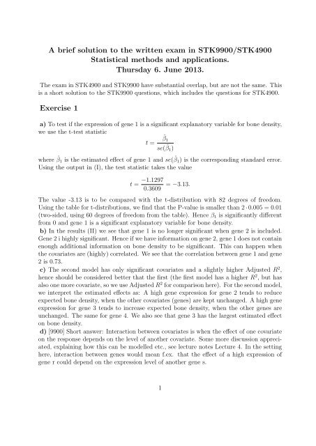
A <strong>brief</strong> <strong>solution</strong> <strong>to</strong> <strong>the</strong> <strong>written</strong> <strong>exam</strong> <strong>in</strong> <strong>STK9900</strong>/<strong>STK4900</strong><br />
<strong>Statistical</strong> methods and applications.<br />
Thursday 6. June 2013.<br />
The <strong>exam</strong> <strong>in</strong> <strong>STK4900</strong> and <strong>STK9900</strong> have substantial overlap, but are not <strong>the</strong> same. This<br />
is a short <strong>solution</strong> <strong>to</strong> <strong>the</strong> <strong>STK9900</strong> questions, which <strong>in</strong>cludes <strong>the</strong> questions for <strong>STK4900</strong>.<br />
Exercise 1<br />
a) To test if <strong>the</strong> expression of gene 1 is a significant explana<strong>to</strong>ry variable for bone density,<br />
we use <strong>the</strong> t-test statistic<br />
t = ˆβ 1<br />
se( ˆβ 1 )<br />
where ˆβ 1 is <strong>the</strong> estimated effect of gene 1 and se( ˆβ 1 ) is <strong>the</strong> correspond<strong>in</strong>g standard error.<br />
Us<strong>in</strong>g <strong>the</strong> output <strong>in</strong> (I), <strong>the</strong> test statistic takes <strong>the</strong> value<br />
t = −1.1297<br />
0.3609 = −3.13.<br />
The value -3.13 is <strong>to</strong> be compared with <strong>the</strong> t-distribution with 82 degrees of freedom.<br />
Us<strong>in</strong>g <strong>the</strong> table for t-distributions, we f<strong>in</strong>d that <strong>the</strong> P-value is smaller than 2 · 0.005 = 0.01<br />
(two-sided, us<strong>in</strong>g 60 degrees of freedom from <strong>the</strong> table). Hence β 1 is significantly different<br />
from 0 and gene 1 is a significant explana<strong>to</strong>ry variable for bone density.<br />
b) In <strong>the</strong> results (II) we see that gene 1 is no longer significant when gene 2 is <strong>in</strong>cluded.<br />
Gene 2 i highly significant. Hence if we have <strong>in</strong>formation on gene 2, gene 1 does not conta<strong>in</strong><br />
enough additional <strong>in</strong>formation on bone density <strong>to</strong> be significant. This can happen when<br />
<strong>the</strong> covariates are (highly) correlated. We see that <strong>the</strong> correlation between gene 1 and gene<br />
2 is 0.73.<br />
c) The second model has only significant covariates and a slightly higher Adjusted R 2 ,<br />
hence should be considered better that <strong>the</strong> first (<strong>the</strong> first model has a higher R 2 , but has<br />
also one more covariate, so we use Adjusted R 2 for comparison here). For <strong>the</strong> second model,<br />
we <strong>in</strong>terpret <strong>the</strong> estimated effects as: A high gene expression for gene 2 tends <strong>to</strong> reduce<br />
expected bone density, when <strong>the</strong> o<strong>the</strong>r covariates (genes) are kept unchanged. A high gene<br />
expression for gene 3 tends <strong>to</strong> <strong>in</strong>crease expected bone density, when <strong>the</strong> o<strong>the</strong>r genes are<br />
unchanged. The same for gene 4. We also see that gene 3 has <strong>the</strong> largest estimated effect<br />
on bone density.<br />
d) [9900] Short answer: Interaction between covariates is when <strong>the</strong> effect of one covariate<br />
on <strong>the</strong> response depends on <strong>the</strong> level of ano<strong>the</strong>r covariate. Some more discussion appreciated,<br />
expla<strong>in</strong><strong>in</strong>g how this can be modelled etc., see lecture notes Lecture 4. In <strong>the</strong> sett<strong>in</strong>g<br />
here, <strong>in</strong>teraction between genes would mean f.ex. that <strong>the</strong> effect of a high expression of<br />
gene r could depend on <strong>the</strong> expression level of ano<strong>the</strong>r gene s.<br />
1
Exercise 2<br />
a) We have data (x 1 , x 2 , y) for n = 35 subjects (surgeries), where x 1 and x 2 are explana<strong>to</strong>ry<br />
vaiables and <strong>the</strong> outcome y is b<strong>in</strong>ary (0 and 1). We are <strong>in</strong>terested <strong>in</strong> modell<strong>in</strong>g <strong>the</strong><br />
probability of gett<strong>in</strong>g a sore throat as a function of <strong>the</strong> explana<strong>to</strong>ry variables, hence we<br />
model p(x 1 , x 2 ) = P (y = 1|x 1 , x 2 ) with a logistic regression model<br />
p(x 1 , x 2 ) = exp(β 0 + β 1 x 1 + β 2 x 2 )<br />
1 + exp(β 0 + β 1 x 1 + β 2 x 2 ) .<br />
This ensures that p(x 1 + x 2 ) is a proper probability, and <strong>the</strong> log odds will be l<strong>in</strong>ear <strong>in</strong> <strong>the</strong><br />
covariates.<br />
b) With only one explana<strong>to</strong>ry variable x 1 , we f<strong>in</strong>d<br />
estimated as<br />
P (y = 1|x 1 = 30) = exp(β 0 + β 1 · 30)<br />
1 + exp(β 0 + β 1 · 30)<br />
exp(−2.21358 + 0.07038 · 30)<br />
1 + exp(−2.21358 + 0.07038 · 30) = 0.4745.<br />
c) The odds ratio for 40 m<strong>in</strong>utes wrt. 30 m<strong>in</strong>utes is exp(10 · ˆβ 1 ) = exp(0.7038) = 2.02 .<br />
A confidence <strong>in</strong>terval for 10 · β 1 is found through<br />
10 · ˆβ 1 ± 1.96se(10 · ˆβ 1 ),<br />
where se(10· ˆβ 1 ) = 10·se( ˆβ 1 ). With <strong>the</strong> estimates from R we get 0.7038±1.96·0.2667, giv<strong>in</strong>g<br />
<strong>the</strong> 95% confidence <strong>in</strong>terval (0.181068, 1.226532). This gives a 95% confidence <strong>in</strong>terval for<br />
<strong>the</strong> odds ratio as<br />
(exp(0.181068), exp(1.226532))<br />
that is, (1.199, 3.409). The OR tells us that <strong>the</strong> odds for a sore throat are doubled if <strong>the</strong><br />
surgery lasts 10 m<strong>in</strong>utes more. From <strong>the</strong> confidence <strong>in</strong>terval we can conclude that <strong>the</strong>re is<br />
some uncerta<strong>in</strong>ty about this doubl<strong>in</strong>g, but at least we can say that <strong>the</strong> odds are <strong>in</strong>creased<br />
(start<strong>in</strong>g above 1).<br />
d) Wald test:<br />
H 0 : β 2 = 0 versus H a : β 2 ≠ 0<br />
From R we f<strong>in</strong>d <strong>the</strong> z-value -1.798, and a P-value= 2P (Z > 1.798) = 2 · 0.036 = 0.072<br />
where Z is standard normal. This P-value is not small enough <strong>to</strong> reject H 0 at level 0.05,<br />
so <strong>the</strong> type (x 2 ) is not significantly improv<strong>in</strong>g <strong>the</strong> model.<br />
Deviance test:<br />
G = D 0 − D = 33.651 − 30.138 = 3.513<br />
G is χ 2 with 1 df under H 0 . From <strong>the</strong> χ 2 table we f<strong>in</strong>d that <strong>the</strong> P-value must be larger<br />
than 0.05, and conclude aga<strong>in</strong> that type (x 2 ) is not significantly improv<strong>in</strong>g <strong>the</strong> model.<br />
2
Exercise 3<br />
a) The estimated rate ratio is exp(1.2016) = 3.325, hence <strong>the</strong> rate of wave caused damages<br />
is more than three times larger for <strong>the</strong> ships built <strong>in</strong> 70-74 compared <strong>to</strong> 60-64.<br />
b) [9900] For an explanation of over dispersion, see lecture notes for Lecture 8. Should<br />
write down <strong>the</strong> overdispersed Poisson regression model, <strong>in</strong>troduc<strong>in</strong>g V ar(Y i ) = φµ i , and<br />
expla<strong>in</strong> that us<strong>in</strong>g <strong>the</strong> quasi family <strong>in</strong> <strong>the</strong> glm allows <strong>to</strong> estimate φ and corrects <strong>the</strong> standard<br />
errors <strong>to</strong><br />
√<br />
se ∗ = se ˆφ.<br />
For <strong>the</strong> ship damage data, ˆφ = 3.19643 and <strong>the</strong> standard errors of <strong>the</strong> estimated coefficients<br />
are scaled up with a fac<strong>to</strong>r<br />
√<br />
ˆφ = 1.788,<br />
and <strong>the</strong> test statistics and p-values corrected correspond<strong>in</strong>gly. The p-values become bigger,<br />
but <strong>the</strong> effects are still significant.<br />
c) This is a Poisson model with observations that are aggregated counts. If Y i is <strong>the</strong><br />
number of counts <strong>in</strong> group i, <strong>the</strong> model can be <strong>written</strong> as<br />
E(Y i ) = exp(log(months i ) + β 0 + β 1 x Bi + β 2 x Ci + β 3 x Di + β 4 x Ei<br />
+β 5 x 65−69,i + β 6 x 70−74,i + β 7 x 75−79,i + β 8 x op75−79,i )<br />
where x Bi = 1 if ship type <strong>in</strong> group i is B and 0 o<strong>the</strong>rwise, etc. We test<br />
us<strong>in</strong>g a deviance test:<br />
H 0 : β 1 = β 2 = β 3 = β 4 = β 8 = 0<br />
G = D 0 − D = 73.225 − 38.695 = 34.53.<br />
G is χ 2 with 5 df under H 0 . P (χ 2 5 > 34.53) < 0.005 and we reject H 0 at any reasonable<br />
level of significance. Hence we can conclude that <strong>the</strong> new variables significantly improve<br />
<strong>the</strong> model.<br />
d) Us<strong>in</strong>g estimated rate ratios, we f<strong>in</strong>d that ship type B, C and D all are safer than ship<br />
type A, when all o<strong>the</strong>r covariates are unchanged. Ship type E is more dangerous.<br />
Specifically we f<strong>in</strong>d RR=exp(-0.6874)=0.5029 for ship type C compared <strong>to</strong> ship type A,<br />
when all o<strong>the</strong>r covariates are unchanged. Similarly we f<strong>in</strong>d RR=exp(-0.5433)=0.5808 for<br />
ship type B compared <strong>to</strong> A. Ship type C has <strong>the</strong>refore <strong>the</strong> lowest rate of wave caused<br />
damage, but <strong>the</strong> standard error of ˆβ 2 is much larger than that of ˆβ 1 , so it is also reasonable<br />
<strong>to</strong> argue that ship type B should be considered <strong>the</strong> safest, given that <strong>the</strong> difference <strong>in</strong> RR<br />
is very small.<br />
The RR for operation <strong>in</strong> <strong>the</strong> last period wrt <strong>the</strong> first is RR=exp(0.38447)=1.4688. This<br />
means that <strong>the</strong>re was an <strong>in</strong>creased risk of damage for operations <strong>in</strong> <strong>the</strong> period 1975-79<br />
compared <strong>to</strong> <strong>the</strong> previous period 1960-74, when all o<strong>the</strong>r covariates as ship type and year<br />
of construction are <strong>the</strong> same.<br />
3