![Question 1 [22 Marks] In the 1974 Motor Trend US magazine, fuel ...](https://img.yumpu.com/27496340/1/500x640/question-1-22-marks-in-the-1974-motor-trend-us-magazine-fuel-.jpg)
Question 1 [22 Marks] In the 1974 Motor Trend US magazine, fuel ...
Question 1 [22 Marks] In the 1974 Motor Trend US magazine, fuel ...
Question 1 [22 Marks] In the 1974 Motor Trend US magazine, fuel ...

Create successful ePaper yourself
Turn your PDF publications into a flip-book with our unique Google optimized e-Paper software.
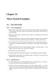
<strong>Question</strong> 1 [<strong>22</strong> <strong>Marks</strong>]<br />
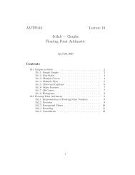
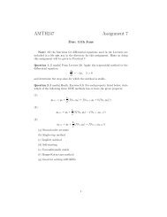
<strong>In</strong> <strong>the</strong> <strong>1974</strong> <strong>Motor</strong> <strong>Trend</strong> <strong>US</strong> <strong>magazine</strong>, <strong>fuel</strong> consumption (mpg in miles/<strong>US</strong> gallon) was related<br />
to several aspects of automobile design and performance for 32 automobiles (1973-74<br />
models). We consider three of <strong>the</strong> variables, displacement (disp in cu.in), horse power (hp)<br />
and weight (wt, lb/1000). The data is plotted below toge<strong>the</strong>r with <strong>the</strong> log transformed<br />
data.<br />
100 300 2 3 4 5<br />
4.5 5.0 5.5 6.0 0.4 0.8 1.2 1.6<br />
mpg<br />
10 15 20 25 30<br />
logmpg<br />
2.4 2.8 3.2<br />
100 300<br />
disp<br />
4.5 5.0 5.5 6.0<br />
logdisp<br />
hp<br />
50 150 250<br />
loghp<br />
4.0 4.5 5.0 5.5<br />
2 3 4 5<br />
wt<br />
0.4 0.8 1.2 1.6<br />
logwt<br />
10 15 20 25 30<br />
50 150 250<br />
2.4 2.8 3.2<br />
4.0 4.5 5.0 5.5<br />
(i) From <strong>the</strong> graphs it was decided to use <strong>the</strong> log transformed variables in <strong>the</strong> analysis.<br />
Explain why you think this may or may not be a good idea.
(ii) The following model was fitted<br />
logmpg = µ + β 1 logdisp + β 2 loghp + β 3 logwt + error<br />
Complete <strong>the</strong> summary of <strong>the</strong> fit that follows by replacing <strong>the</strong> ∗’s.<br />
Coefficients:<br />
Estimate Std. Error t value Pr(>|t|)<br />
(<strong>In</strong>tercept) 4.9462 0.2687 18.41
<strong>Question</strong> 2 [30 <strong>Marks</strong>]<br />
(This question has been modified as <strong>the</strong> original question was not suitable for <strong>the</strong> unit as<br />
presented in 2002.)<br />
The original data set in question 1 also contains <strong>the</strong> number of cylinders (cyl: 4, 6 or 8) for<br />
each car tested. Since it is quite possible <strong>the</strong> relationship between mpg and displacement<br />
will also depend on <strong>the</strong> number of cylinders it was decided to examine this relationship<br />
separately.<br />
Miles/<strong>US</strong> gallon<br />
10 15 20 25 30<br />
four<br />
six<br />
eight<br />
100 200 300 400<br />
displacement<br />
The following models were fitted and <strong>the</strong> output from R is reported:<br />
Model 1: (3 intercepts and 3 slopes)<br />
Analysis of Variance Table<br />
Response: mpg<br />
Df Sum Sq Mean Sq F value Pr(>F)<br />
cyl 2 824.78 412.39 73.3<strong>22</strong>1 2.050e-11<br />
disp 1 57.64 57.64 10.2487 0.003591<br />
cyl:disp 2 97.39 48.69 8.6574 0.001313<br />
Residuals 26 146.23 5.62
Model 2: 3 intercepts, 1 common slope (parallel lines).<br />
Analysis of Variance Table<br />
Response: mpg<br />
Df Sum Sq Mean Sq F value Pr(>F)<br />
cyl 3 13741 4580 526.434 |t|)<br />
(<strong>In</strong>tercept) 40.87196 3.02012 13.533 2.79e-13<br />
cyl6 -21.78997 5.30660 -4.106 0.000354<br />
cyl8 -18.83916 4.61166 -4.085 0.000374<br />
disp -0.13514 0.02791 -4.842 5.10e-05<br />
cyl6:disp 0.13875 0.03635 3.817 0.000753<br />
cyl8:disp 0.11551 0.02955 3.909 0.000592<br />
Residual standard error: 2.372 on 26 degrees of freedom<br />
Multiple R-Squared: 0.8701, Adjusted R-squared: 0.8452<br />
F-statistic: 34.84 on 5 and 26 DF, p-value: 9.968e-11<br />
(a) Write down <strong>the</strong> equation of <strong>the</strong> three lines.<br />
(b) Test whe<strong>the</strong>r <strong>the</strong> slopes of <strong>the</strong> lines for <strong>the</strong> 6 and 8 cylinder cars are different<br />
from <strong>the</strong> slope of <strong>the</strong> line for <strong>the</strong> 4 cylinder cars.<br />
(c) Verify <strong>the</strong> 95% CI for <strong>the</strong> slope of <strong>the</strong> line for four cylinder cars is given by<br />
(−0.193, −0.078).<br />
(d) If <strong>the</strong> 95% CI for <strong>the</strong> slope of <strong>the</strong> line for six cylinder cars is (−0.044, 0.051)<br />
and that for eight cylinder cars is (−0.040, 0.0003) what can you say about <strong>the</strong><br />
relationship of <strong>the</strong> slopes of <strong>the</strong> three lines?
(iii) The mpg was estimated for cars with a displacement of 150 cu.in and having 4, 6<br />
and 8 cylinders using R.<br />
$fit<br />
1 2 3<br />
* 19.6<strong>22</strong>8 19.0877<br />
$se.fit<br />
1 2 3<br />
1.44190 1.18564 2.07059<br />
Comment on <strong>the</strong> results after first replacing <strong>the</strong> missing value (for 4 cylinder cars).<br />
(iv) With <strong>the</strong> aid of <strong>the</strong> following plots comment on <strong>the</strong> assumptions for <strong>the</strong> model and<br />
<strong>the</strong> fit of <strong>the</strong> line.<br />
Residual Plot<br />
Normal Q−Q Plot<br />
Residual<br />
−2 0 2 4<br />
Sample Quantiles<br />
−2 0 2 4<br />
15 20 25 30<br />
Fitted<br />
−2 −1 0 1 2<br />
Theoretical Quantiles
<strong>Question</strong> 3 25 <strong>Marks</strong>]<br />
An animal experiment is designed to investigate whe<strong>the</strong>r levorphanol reduces stress as<br />
reflected in <strong>the</strong> cortical sterone level. There were four treatment groups containing five<br />
animals each. The four treatments consisted of a control (C), levorphanol only (L),<br />
epinephrine only (E), and levorphanol plus epinephrine (LE).<br />
(i) Complete <strong>the</strong> ANOVA table below.<br />
Analysis of Variance Table<br />
Response: cs<br />
Df Sum Sq Mean Sq F value Pr(>F)<br />
treat * 37.58 * * 2e-04<br />
Residuals 16 16.30 *<br />
(ii) Write down and test a suitable hypo<strong>the</strong>sis concerning treatments.<br />
(iii) Write down three contrasts to test<br />
(a) The main effect of levorphanol (levor)<br />
(b) The main effect of epinephrine (epin)<br />
(c) <strong>the</strong> interaction between levorphanol and epinephrine (levor:epin).<br />
(iv) Show <strong>the</strong> contrasts are orthogonal to each o<strong>the</strong>r.
(v) Using <strong>the</strong> following ANOVA table and table of means, write down and test hypo<strong>the</strong>ses<br />
concerning <strong>the</strong> main effects of levorphanol, epinephrine and <strong>the</strong>ir interaction.<br />
Analysis of Variance Table<br />
Response: cs<br />
Df Sum Sq Mean Sq F value Pr(>F)<br />
levor 1 12.832 12.832 12.598 0.002670<br />
epin 1 18.586 18.586 18.246 0.000584<br />
levor:epin 1 6.161 6.161 6.048 0.025692<br />
Residuals 16 16.298 1.019<br />
Tables of means<br />
Grand mean<br />
2.964<br />
levor<br />
0 1<br />
3.765 2.163<br />
epin<br />
0 1<br />
2.000 3.928<br />
levor:epin<br />
epin<br />
levor 0 1<br />
0 2.246 5.284<br />
1 1.754 2.572<br />
Standard errors for differences of means<br />
levor epin levor:epin<br />
0.4514 0.4514 0.6383<br />
replic. 10 10 5<br />
(vi) Write a conclusion.
<strong>Question</strong> 4 [20 <strong>Marks</strong>]<br />
An experiment is conducted to determine <strong>the</strong> effect of three levels of fertilization on <strong>the</strong><br />
yield of sugar cane. The experiment is conducted at four locations, randomly selected<br />
from a number of possible locations available for <strong>the</strong> experiment. Each fertilizer level is<br />
applied to three plots at each location.<br />
(i) Complete <strong>the</strong> following table<br />
Df Mean Sq Expected Mean Square F P<br />
fertilizer * 12.15514 * * *<br />
location * 4.60598 * * *<br />
fertilizer:location * 0.15544 * * *<br />
Residuals 24 0.05793<br />
(Note <strong>the</strong> Sum of Squares column has been omitted and is not needed.)<br />
(ii) Write down and test appropriate hypo<strong>the</strong>ses concerning fertilizer treatments, locations<br />
and <strong>the</strong> interaction between fertilizer treatment and location.<br />
(iii) Estimate <strong>the</strong> components of variation.<br />
(iv) Calculate <strong>the</strong> variation of a single observation.<br />
(v) The fertilizer SS is partitioned using polynomial contrasts. The significance levels<br />
are given for <strong>the</strong> resulting F values in <strong>the</strong> ANOVA table.<br />
Analysis of Variance Table<br />
Response: yield<br />
Pr(>F)<br />
linear<br />
3.32e-05<br />
quadratic<br />
1.65e-11<br />
location<br />
1.31e-12<br />
location:fertilizer 0.0389<br />
<strong>In</strong>terpret <strong>the</strong>se results with <strong>the</strong> aid of <strong>the</strong> following table of mean yields for <strong>the</strong> three<br />
fertilizer levels.<br />
1 2 3<br />
16.7567 17.9208 15.9167<br />
(vi) Write a conclusion.